Boundary slip and nanobubble study in micro/nanofluidics using atomic force microscopy
Yuliang
Wang
ab and
Bharat
Bhushan
*a
aNanoprobe Laboratory for Bio- & Nanotechnology and Biomimetics (NLB2), The Ohio State University, 201 W. 19th Avenue, Columbus, OH 43210-1142, USA. E-mail: Bhushan.2@osu.edu
bMechanical Engineering, Harbin Institute of Technology, Harbin, 150001, P.R. China
First published on 24th November 2009
Abstract
The boundary condition at the solid–liquid interface on the micro/nanoscale is an important issue in micro/nanofluidic systems, where drag forces between fluids and solid walls need to be minimized. Recent studies have shown that on hydrophobic surfaces the fluid velocity near the solid surface is not equal to the velocity of the solid surface, a phenomenon called boundary slip. Theoretical and experimental studies suggest that at the solid–liquid interface, the presence of nanobubbles is responsible for boundary slip. In this review, various techniques for boundary slip investigation are described. We focus on the research performed using contact and tapping mode atomic force microscopy methods to study boundary slip on hydrophilic, hydrophobic, and superhydrophobic surfaces. The impact of surface roughness and hydrophobicity on measured slip length is discussed. The process of how to eliminate the influences of cantilever deflection and electrostatic forces on experimental measurement is discussed. Based on nanobubble imaging on a hydrophobic surface, the role of nanobubbles on boundary slip is discussed. Nanobubble movement and coalescence, as well as tip–nanobubble interactions, are discussed. The relationship between nanobubble immobility and surface structures on hydrophobic surfaces is discussed. Finally, a method to quantitatively measure sliding force on hydrophobic surfaces using atomic force microscopy is presented, and the effect of the presence of an electric field is discussed.
 Yuliang Wang | Yuliang Wang has been pursuing a PhD degree in Mechanical Engineering at the Harbin Institute of Technology since 2004. He received his B.S. (2004) in Mechanical Engineering from the Harbin Institute of Technology. From Sep. 2005 to Aug. 2006, he has been a visiting scholar at Hanyang University and Korean Institute of Science and Technology, Korea. From Sep. 2007 to Aug. 2009, he has been a visiting scholar at the Ohio State University, OH, USA. His current research is focused on boundary slip studies at the solid–liquid interface in micro/nanofluidics, nanobubble characteristics, micro/nanoscale manipulation, micro/nanotribology studies using atomic force microscopy. |
 Bharat Bhushan | Dr Bharat Bhushan is an Ohio Eminent Scholar and the Howard D. Winbigler Professor in the College of Engineering, and the Director of the Nanoprobe Laboratory for Bio- & Nanotechnology and Biomimetics (NLB2) at the Ohio State University, Columbus, Ohio. He holds two M.S., a PhD in mechanical engineering/mechanics, an MBA, and three semi-honorary and honorary doctorates. His research interests include fundamental studies with a focus on scanning probe techniques in the interdisciplinary areas of bio/nanotribology, bio/nanomechanics and bio/nanomaterials characterization, and applications to bio/nanotechnology and biomimetics. He has authored 6 scientific books, more than 90 handbook chapters, more than 700 scientific papers and more than 60 scientific reports, edited more than 45 books, and holds 17 U.S. and foreign patents. He is the recipient of numerous prestigious awards and international fellowships. |
1. Introduction
The description of fluid dynamics relies on the accurate understanding of the boundary condition at solid–liquid interfaces, especially when the length scale is down to the micro/nanoscale. Finding the actual boundary condition at solid–liquid interfaces is not only of great importance for fundamental research in fluid mechanics, but will also help to improve the fluid dynamics related practical applications, in particular, micro/nanofluidics based biosensor applications. For example, Fig. 1 shows a wrist type biosensor.101 In micro/nanofluidics systems, microchannels are widely used to transport fluids and chemical agents. In the microchannels, because of a larger surface to volume ratio, the drag force between fluid flow and solid walls becomes an important issue and needs to be minimized.7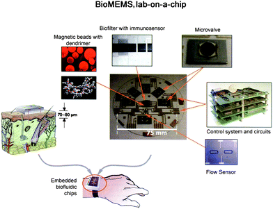 | ||
| Fig. 1 An example of a wrist type biosensor.101 | ||
The majority of problems in fluid dynamics are described with two differential equations, referred as the Navier–Stokes equations, and generally resolved with the no-slip boundary condition.99,2 In the no-slip boundary condition, it is assumed that the relative velocity between a solid wall and liquid flow is zero at the solid–liquid interfaces. Although the no-slip boundary condition is an assumption and cannot be proven with hydrodynamic theories, it still forms the basis of continuum fluidics. However, recent studies have shown that on hydrophobic surfaces, fluid flow exhibits a phenomenon known as boundary slip, which means that the fluid velocity near the solid surface is not equal to the velocity of the solid surface41,42,61,78,67 and hence reduces drag in fluid flow. Therefore, the study of boundary slip is of great interest to micro/nanofluidics applications.
Regarding the mechanism of the existence of boundary slip, air bubbles on the nanoscale (referred as nanobubbles) are considered to be the reason. During wetting of a hydrophobic surface with an aqueous solution, spherical cap nanobubbles with dimensions of 5–100 nm in height and 50–800 nm in diameter are produced using tapping mode atomic force microscopy (TMAFM).48,65,106,44,95,12 Nanobubble studies are of great interest to both theoretical research and practical applications of interactions between hydrophobic surfaces and aqueous solutions, which have been extensively studied over several decades. From a theoretical research aspect, nanobubbles on hydrophobic surfaces are considered to be the cause for the observed long-range (10–100 nm) attractive forces,26,48,32,90,106,52 which was first indicated by Israelachvili and Pashley,50 and was found to be greater in magnitude than the van der Waals force. When two hydrophobic surfaces approach each other, the coalescence of nanobubbles between two surfaces will form a gas bridge and lead to the long-range attractive force. From a practical application point of view, theoretical studies60,34,91 and experimental studies81,54 suggest that at the solid–liquid interface, the presence of nanobubbles is responsible for the apparent slip or, more specifically, the breakdown of the no-slip boundary condition for hydrophobic surfaces. Nanobubbles decrease the solid–liquid interaction and hence reduce friction between fluid and solid walls at the solid–liquid interfaces. Therefore, the study of nanobubbles will provide an approach to reduce drag forces during liquid transportation on the micro/nanoscale.
Generally speaking, both the boundary slip at solid–liquid interfaces and nanobubble formation are correlated with surface properties, in particular, wettability and surface roughness. Therefore, surfaces with designed wettability are supposed to have potential applications in boundary slip and nanobubble studies. Advances in nanotechnology have stimulated the development of surfaces with desirable wettability.7 Micro/nanopatterned or hierarchical structures on hydrophobic surfaces can be fabricated to achieve superhydrophobic surfaces with static contact angles larger than 150°.9,79,14 The combination of surface modification with boundary slip and nanobubble studies will greatly accelerate the development of micro/nanofluidics. In this section, a history of boundary slip at solid–liquid interfaces and our current understanding of nanobubbles on hydrophobic surfaces will be separately provided.
1.1 History of boundary slip studies
The actual boundary condition at solid–liquid interfaces in fluid dynamics has been widely debated since the 19th century. To describe the motion of fluid flow over a solid surface, instead of Navier–Stokes equations,99 the boundary condition at the solid–liquid interface is required for solutions. No-slip and slip boundary conditions have been proposed to study fluid dynamics at different times in the 18th and 19th centuries.41 Bernoulli4 first stated that there is no relative movement between fluid flows and solid walls, referred as a no-slip boundary condition, as shown in Fig. 2a. The velocity of fluid flow gradually decreases to zero at a solid–liquid interface. In the slip boundary condition, which was first proposed by Navier77 and later by Maxwell,72 the tangential velocity of fluids is proportional to the ratio of the velocity to the velocity gradient in a direction perpendicular to the solid walls, as | (1) |
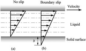 | ||
| Fig. 2 Velocity profiles of liquid between two parallel planar plates assuming there is no slip at the solid–liquid interface of the top plate. The top plate moves rightward and shears the liquid. The velocity gradually diminishes to zero if there is no slip at bottom plate (a). When boundary slip occurs at the solid–liquid interface on the bottom plate with slip length b, there is relative velocity between fluid flow and the plate (b). | ||
Both no-slip and slip boundary conditions have had their supporters since the 18th century. Du Buat38 (1796) experimentally confirmed the no-slip boundary condition by driving water flow through pipes. Stokes98 tried to reveal the true nature of the boundary condition between Bernoulli's no-slip boundary condition and Navier's slip boundary condition hypotheses. He finally supported the no-slip boundary condition based on the motivation that any discontinuity in velocity between a fluid flow and a solid wall would give rise to a tangential force which will immediately destroy the finite relative motion. After that, experimental results of water and mercury flowing through glass pipes supported Stokes' study with a no-slip boundary condition.117,109 However, several other experimental results were consistent with the slip boundary condition. Shortly after the slip boundary condition was proposed by Navier.77 Helmholtz and Pictowsky43 found experimental evidence of boundary slip for a liquid flowing over a solid surface and found a considerable slip for water flow on a gold coated surface. Later, Traube and Whang103 reported a great reduction of time used for water flowing through a capillary tube at low pressure after they treated the tube with oleic acid or other polar organic compounds. Schnell93 observed flow rate driven by various pressures through glass capillary tubes with and without hydrophobic treatment with the vapor of dimethyldichlorosilane. He found that at low driving pressure, the flow rate was lower for treated tubes than that of untreated ones because of surface tension effects. However, the flow rate finally became greater than that of the untreated tubes in treated ones with increasing pressure due to boundary slip at solid-liquid surfaces in hydrophobic treated tubes. Churaev et al.33 compared flow rates of water and carbon tetrachloride through hydrophobized silica microcapillaries and reported that the flow rate of water was greater than for the completely wetting CCl4, with the discrepancy corresponding to a slip length of about 30 nm, which implies a strong correlation between surface hydrophobicity and boundary slip at solid–liquid interfaces.
In his book, Goldstein41 stated that “slip, if it takes place, is too small, or a quasi-solid layer of fluid, if there is one, is too thin, to be observed or to make any observable difference in the results of the theoretical deductions.” However, the appearances of novel experimental devices and techniques, such as the surface force apparatus (SFA) and atomic force microscopy (AFM), make it possible to control systems on the micro/nanoscale and open ways to investigate boundary conditions in a small length scale never done before. Moreover, the rapid development of micro/nanoscale fabrication techniques combined with biology and life science has stimulated the development of micro/nanofluidics.7 Now it is generally accepted that boundary slip occurs on hydrophobic surfaces, and on hydrophilic surfaces, the no-slip boundary condition is generally satisfied.
Recently, liquid drainage experiments with more advanced techniques of SFA,3,126,35 particle image velocimetry (PIV),104 and AFM112 reported slip length on hydrophobic surfaces, and no slip was observed on hydrophilic surfaces.3,104,112,35,45,114,15,68 These experimental results are consistent with the molecular dynamic (MD) simulation results performed by Barrat and Bocquet,1 who obtained 30 molecular diameters' slip length on a surface with a contact angle of 140°, while no slip was observed on hydrophilic surfaces. However, boundary slip is also reported on hydrophilic surfaces in other experiments, such as SFA,125 AFM,36,16 PIV53 and TIR-FRAP methods (total internal reflection–fluorescence recovery after photobleaching).83,92 These unexpected data have something to do with sample preparation and data analysis. For example, electrostatic double-layer force and Stokes friction exists in experimental data and needs to be subtracted, as stated by Wang et al.114
Wang et al.114 and Maali et al.68 studied boundary slip on hydrophilic, hydrophobic, and superhydrophobic surfaces with contact mode AFM. They demonstrated how to eliminate the influence of cantilever deflection impact on actual separation distance and approach velocity, as well as the impact of electrostatic double-layer force between the sphere and solid surface and the Stokes friction component on cantilever deflection. In order to obtain actual separation distance, the cantilever deflection was added to the PZT vertical displacement. The actual approach velocity is then obtained from the real sphere–surface separation distance by differentiating the real sphere–surface separation distance. The deflection component generated by the electrostatic double-layer force was determined by performing drainage experiments with two very low approach velocities (0.4 and 0.8 μm s−1). They found that the slip length value is independent of approaching velocity up to 56 μm s−1. To eliminate the influence of surface roughness of the superhydrophobic surface on boundary slip, they took the mean surface as a virtual plane where the solid–liquid interface is located. They got a no-slip boundary condition for a glass sphere on the hydrophilic surface, while there is about 44 and 257 nm slip lengths on the hydrophobic and superhydrophobic surfaces, respectively.
Later, Bhushan et al.15 studied boundary slip on these surfaces with TMAFM. In TMAFM, amplitude and phase signal are obtained while the oscillating sphere approaches the solid surface at a low velocity. Therefore, the deflection signal remains constant and can be taken as an indicator to determine actual contact position within a resolution of 1 nm. Slip lengths of about 43 and 236 nm are obtained on hydrophobic and superhydrophobic surfaces, which indicates that the slip length increases with increasing hydrophobicity. However, based on experimental measurements performed by Cho et al.,29 polarity of liquids also influences boundary slip. During measuring various polar liquids on alkylsilane coated glass surfaces, the slip lengths were found to decrease with increasing dipolar moment of the liquids.29 They proposed that a lattice structure generated by dipole–dipole and dipole–image dipole interactions is responsible for the slip behavior. With increasing dipole moment, the cohesive energy of the lattice structure increases, thus it is difficult to shear liquid at the solid–liquid interface which shows up as a decreasing slip length.
1.2 Nanobubbles on hydrophobic surfaces
The existence of nanobubbles has been detected by various techniques, such as TMAFM,48,65,106,44,95,12 rapid cryofixation/freeze fracture,100 neutron reflectometry,97 spectroscopic method,124 and X-ray reflectivity measurements.86 Molecular dynamics (MD) simulations have also been used to explain the existence of nanobubbles.57 However, the most popular tool for nanobubble study is TMAFM. In TMAFM, an oscillating tip intermittently contacts the sample surface with a much lighter force exerted on the sample than in contact mode AFM.8 Thus, the technique is widely used to detect soft and fragile materials either in an ambient circumstance or in liquid. The nanobubbles generally appear to be long-lived, with lifetimes over 20 h121 and are stable not only under ambient conditions but also under enormous reduction of the water pressure down to −6 MPa.18 In TMAFM, coalescence and movement of nanobubbles can occur under perturbation of AFM tips.121,95,12 By tracking the movement of nanobubbles and the consequent coalescence during scanning with TMAFM, Bhushan et al.12 have shown that small nanobubbles are first moved and merged into big nanobubbles, leading to the formation of larger nanobubbles. They calculated the volumes for nanobubbles before and after coalescence and further confirmed that the spherical objects that appear on hydrophobic surfaces are indeed nanobubbles.In addition to the spontaneous generation of nanobubbles on hydrophobic surfaces,12 nanobubbles can also be generated through the exchange of liquids with different gas solubility on hydrophilic surfaces, for example ethanol and water.65,122 After initial exposure of the hydrophilic surface to ethanol, nanobubbles were formed after the surrounding liquid was switched from ethanol to water. Additionally, experimental results show that both the dissolved gases and liquid temperature are important for the formation of nanobubbles.122 When the liquids were degassed, the number of nanobubbles decreased comparable to that obtained by the nondegassed liquids. Regarding liquid temperature, Zhang et al.122 found that the density of nanobubbles increased with the liquid temperature. When the liquid temperature was over 30 °C, the density of nanobubbles showed a rapid growth.
Nanobubbles provide an approach to detect solid–liquid contact on the nanoscale. Bhushan et al.12 and Wang et al.115 studied cantilever tip–nanobubble interactions through force modulation curves in TMAFM and force curves in contact mode AFM, respectively. By using force modulation curves, nanobubble height and tip–nanobubble adhesion information can be extracted. Moreover, interaction stiffness and damping coefficient can be obtained with the amplitude and phase signal.12 By using force curves in contact mode AFM, contact angle hysteresis and solid–liquid contact on the nanoscale is studied.115
The presence of nanobubbles also influences the substrate supporting them. The phenomenon of nanobubble induced nanoindents on hydrophobic polystyrene (PS) films in water was recently investigated by Wang et al.116 After an immersion time for a PS film of over 220 min in water, small nanobubbles gradually diminish and finally disappear, leaving nanoindents. Rim structures appear around bigger nanobubbles. They state that the high inner pressure of nanobubbles combined with the surface tension force around solid–liquid–gas (three phase) contact line leads to the nanoindents under the nanobubbles on the PS film.
From the point of reducing friction force between fluids and solid walls, it is desirable that nanobubbles stay on the hydrophobic surfaces with limited or no movement. This nanobubble immobility is proposed by Wang et al.115 They investigated the influence of surface structures on nanobubble immobility and found that both nanoindents on continuously coated PS films and hydrophobic island structures on partially coated PS films can improve nanobubble immobility. A model based on contact angle hysteresis and surface tension force was also derived to explain the mechanism of improved immobility on both surfaces. They found the initial force needed to move a nanobubble on both nanoindent and island structures is larger than that on a smooth surface.
1.3 Liquid micro droplet sliding
The rapid development of micro/nanoscale fabrication techniques combined with biology and life science have stimulated the development of techniques for transportation and manipulation of fluids on the microscale.7 One way to transport fluids is to slide liquid droplets over surfaces by generating a gradient of wettability,27,47,37 a driving force based on molecular absorption by selection of the molecular structure of the incorporated adsorbates,62 or dielectrophoretic forces which attract polarizable objects to areas of high field intensity in an alternating or constant electric field.108 On the microscale, surface forces, especially capillary forces, become dominant compared with the gravitational force and can be applied to micromanipulation by forming a liquid bridge between a probe and target objects.80,58,89,11 In addition to the practical applications just mentioned, liquid droplet sliding is also instructive to evaluate the degree of boundary slip on hydrophobic and superhydrophobic surfaces of interest in micro/nanofluidics. The existence of boundary slip can reduce drag in fluid flow, which is particularly meaningful in micro/nanofluidics.In micro/nanofluidics based biosensor applications, polymers are widely used. The effect of surface charge on fluid flows on the micro/nanoscale is of interest to both droplet sliding and boundary slip studies. It is well known that the wettability of conducting liquids on a dielectric layer between two electrodes can be controlled by applying an electric field between the electrodes, called electrowetting.87,76 The presence of the electric field reduces the interface tension between the liquid and the substrate, leading to a reduction of the contact angle and enhancing the wettability of the liquid.10 Since the contact angle and interface tension of liquid droplets can be tuned locally with applied potentials, electrowetting has been intensively used to study the sliding of fluid droplets by switching potentials applied on designed configuration of electrodes.85,30 Regarding boundary slip study, an electric field is expected to affect the fluid flow by changing the interaction between liquid and solid surfaces.
Current research mainly focuses on the realization of liquid motion. The driving forces are seldom measured, especially when potentials are applied to the droplets and the substrate electrodes. The measurement of sliding forces is of significance for liquid manipulation related micro/nanofluidics applications. The measurement of sliding forces can provide evidence for the quantitative evaluation of the capability of liquid droplet sliding on specified surfaces. Recently, Wang and Bhushan113 came up with a method of quantitative measurement of liquid droplet sliding force using atomic force microscopy. Micromanipulation was performed to line up micro droplets with different sizes by an AFM tip. The forces needed to slide droplets were measured. To study the effect of electric field on liquid droplet sliding, the sliding force was measured for each droplet with electric potentials applied between AFM tip and sample surface.
1.4 Objectives of the paper
In this review, the recent developments in boundary slip and nanobubble studies, as well as liquid micro droplet sliding in the presence of an electric field, are summarized based on the published literature. Techniques for boundary slip investigation will be briefly described. For a detailed description and comparison of different boundary slip investigation techniques, readers are referred to a review paper by Neto et al.78 In this review paper, we focus on the research performed using contact and tapping mode AFM methods to study boundary slip on hydrophilic, hydrophobic, and superhydrophobic surfaces in deionized (DI) water. The impact of surface roughness and hydrophobicity on measured slip length is discussed. The process of how to eliminate the influences of cantilever deflection and electrostatic forces on experimental measurement is presented. Based on nanobubble imaging on a hydrophobic surface after immersion in DI water, the role of nanobubbles on boundary slip is discussed. Nanobubble movement and coalescence, as well as tip–nanobubble interaction, are discussed. The relationship between nanobubble immobility and surface structures on hydrophobic surfaces is discussed.This review is divided into six sections. In section 2, several techniques to investigate the boundary condition at solid–liquid interfaces will be introduced. The detailed process of AFM measurement of boundary slip will also be mentioned. In section 3, experimental results of boundary slip studies with both contact and tapping mode AFM on hydrophilic, hydrophobic, and superhydrophobic surfaces will be introduced in detail. In section 4, nanobubble imaging, nanobubble–substrate interaction, and tip–nanobubble interaction studies with AFM will be reported. In section 5, liquid micro droplet sliding in the presence of an electric field is studied with AFM as an approach to transport liquids and to investigate solid–liquid interaction. Finally in section 6, an outlook is provided.
2. Measurement techniques for boundary slip
As mentioned earlier, whether or not a boundary slip exists for a given system can vary with the measurement techniques. According to the working principle used, the techniques can be divided into the capillary method, fluid flow tracing method, and liquid drainage method. In this section, these different measurement techniques will be briefly introduced.2.1 Capillary method
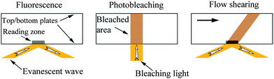
In the capillary method,93,33,81 a liquid in a thin capillary pipe or channel is driven by external pressure at one end. By measuring the pressure drop between the two ends of the pipe and the flow rate, the degree of boundary slip at the solid–liquid interface in the pipe can be investigated. Boundary slip will increase the flow rate for a given pressure drop. By applying the Navier slip boundary condition, the relationship between slip length b, volume flow rate q, and pressure drop Δp between two infinite parallel plates can be given as81,55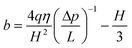 | (2) |
The capillary method is easy to use, and no elaborate equipment is required. However, the pressure drop is difficult to measure. The fluid flow type close to inlets and outlets is different from the steady fluid flow in the central part of a pipe. Therefore, pressure needs to be measured at the central part of a pipe, which is difficult to perform, especially when the size of the pipe is small. Additionally, uniform geometry throughout a pipe is generally difficult to achieve.
2.2 Fluid flow tracing method
In the fluid flow tracing method, the fluid flow is directly observed by using either optical traceable particles or fluorescent molecules as velocity probes. According to the type of velocity probes used, the fluid flow tracing method can be divided as TIR-FRAP method75,82,83,92 and PIV method.73,119,104,53Migler et al.75 first used the fluorescence recovery method as a direct method to measure local velocity of a sheared polymer melt from the solid–liquid interface. In this method, fluorescent probes are put between two planar substrates, as shown in Fig. 3. A low power evanescent wave beam excites the fluorescent probes to give a reference fluorescent intensity value in a reading zone. The reading zone is a liquid cylinder normal to the bottom plate and illuminated by the evanescent wave beam with penetration depth about 100 nm, as labeled in Fig. 3 (left). After that, a high power vertical beam photobleaches the probes for a short time, and the top planar substrate begins to move to bring the photobleached probes away with fluid flows. Meanwhile, the new probes are brought into the reading zone, and the intensity value is thus recovered back to the reference value. By monitoring the fluorescence intensity, the velocity at the wall can be observed.82 The TIR-FRAP method provides direct evidence of the flow rate of shearing fluid. However, the degree of boundary slip is obtained through comparing the fluorescence recovery rate on different surfaces. Additionally, fluorescence molecular diffusion should also be taken into account because of the small size.
 | ||
| Fig. 3 Schematic of TIR-FRAP measurement of boundary condition of fluid flow between two planar plates. An evanescent wave is first used to excite the fluorescent probes to give a reference fluorescent intensity value (left). Then a high power vertical beam photobleaches the probes for a short time (middle). Meanwhile, the top planar substrate begins to move to bring the photobleached probes away with fluid flows, and the new probes are brought into the reading zone, and the intensity value is thus recovered back to the reference value (right). By monitoring the fluorescence intensity, the velocity at the wall is observed. | ||
Another fluid flow tracing method is the PIV method.73,119,104,53 As shown in Fig. 4, in the PIV method, small particles are distributed in fluid flowing through a channel. Movement of fluid flow will bring particles along the flow direction. By monitoring the movement of particles in the area of interest during a certain period of time, the velocity field of the local fluid is determined. PIV method can be used to directly observe the velocity field and then get the slip length value. However, the size of the particles used is restricted with laser wavelength. Moreover, the resolution in determination of solid–liquid interface and particle positions is low. Like in the TIR-FRAP method, particle diffusion effect needs to be considered, especially when the particle size is small.
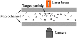 | ||
| Fig. 4 Schematic of PIV measurement of boundary condition in a microchannel. Optically traceable particles are distributed in the channel and brought with fluid flow. The particles in the interest area are illuminated by a laser beam, and the movement of the particles is monitored by a camera, through which the velocity field of fluid flow is observed. | ||
2.3 Liquid drainage method
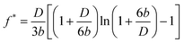
Another popular method to investigate boundary slip is the liquid drainage method using SFA or AFM. The principle of this method is to measure the hydrodynamic drainage force between two crossed cylindrical surfaces (SFA) or a sphere and a planar surface (AFM) as a function of the separation distance when the surfaces approach each other. Under the assumption of the no-slip boundary condition, the hydrodynamic force acting on cylindrical surfaces or the sphere is given as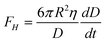 , where η is the viscosity of the liquid, D is the closest separation distance between different surfaces at each case, and dD/dt is the velocity of different surfaces approaching each other. In order to take the boundary slip at solid–liquid interfaces into account, Vinogradova111 developed the relationship for hydrodynamic force. By solving the continuity equation and the Navier–Stokes equation (also known as the momentum equation) of fluid flow in the gap and using the Navier boundary condition of eqn (1), she came up with a modified model for hydrodynamic force for the case of slip boundary condition, given as111
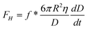 | (3) |
 | (4) |
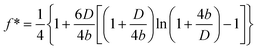
For the case that boundary slip occurs at both surfaces with the same slip length b, the correction parameter is given as
 | (5) |
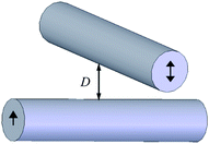 | ||
| Fig. 5 Schematic of SFA measurement of boundary condition between two crossed cylindrical surfaces. The slip length is obtained with the hydrodynamic force and separation distance simultaneously measured during approaching to each other. | ||
2.3.2.1 Contact mode AFM method. In contact mode AFM method, as shown in Fig. 6a, a glass sphere with radius R, which is glued to the end of an AFM cantilever, approaches a solid surface at a relatively large velocity.114,68 Liquid between the sphere and the surface is squeezed out of the gap. The liquid velocity profiles near the solid–liquid interface vary with different boundary conditions, as shown in Fig. 6c. If there is no slip at the interface, the liquid velocity will gradually reduce to zero. Otherwise, there will be a relative velocity between liquid flow and the solid surface when boundary slip exists at the interface. During approaching or retracting movement, the fluid is squeezed out of (or into) the gap, which will lead to hydrodynamic forces exerted on the sphere. The hydrodynamic forces can be measured by multiplying the AFM cantilever's deflection signal with the cantilever stiffness. From eqn (3), one can see that the hydrodynamic force is proportional to the approach velocity dD/dt and inversely proportional to D. The separation distance between the sphere and the solid surface can be recorded. Using eqn (3) to (5), the slip length can be obtained with the obtained hydrodynamic force and separation distance.
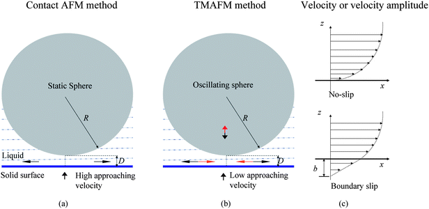 | ||
| Fig. 6 Schematic of a sphere approaching a surface in contact mode AFM (a) and TMAFM (b) measurement of boundary slip and profiles of velocity or amplitude of velocity (c) of fluid flow with and without boundary slip. The definition of slip length b characterizes the degree of boundary slip at the solid–liquid interface. The arrows above and below the solid surface represent directions for fluid flow and relative movement of sample surface to the sphere, respectively.114,15 | ||
In order to get slip length b, a nonlinear least-square fitting method is used to fit hydrodynamic force data with eqn (3) and (4) or (3) and (5), based on the hydrophobicity of spheres and planar surfaces. In eqn (3) to (5), the viscosity η and radius R are known or can be measured. Separation distance D and velocity dD/dt can be obtained with experimental data. Therefore, the only parameter that needs to be determined is slip length b.
Before fitting, one should do some processing of experimental data to eliminate the influence of several factors:114 cantilever deflection impact on the actual separation distance and approach velocity, and the impact of electrostatic double-layer force between the sphere and solid surface and the Stokes friction component16 on cantilever deflection. In order to obtain the actual separation distance, the cantilever vertical deflection was added to the PZT vertical displacement. The actual approach velocity is then obtained from the real sphere–surface separation distance by differentiating the real sphere–surface separation distance.
To measure the electrostatic double-layer force, experiments can be conducted at two very low velocities in order to minimize the hydrodynamic force so that the force measured is dominated by the electrostatic force.114,68 The cantilever deflection signal obtained from two different velocities can be given as:
| S1 = Shydro_1 + Selec | (6) |
| S2 = Shydro_2 + Selec | (7) |
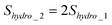 | (8) |
In order to measure the Stokes friction component, the sphere was retracted to be far away from the surface (over 20 μm), where the cantilever deflection is independent of PZT displacement, and the cantilever deflection signal obtained can be regarded as generated by Stokes friction. After the actual separation distance is obtained, and the electrostatic double-layer and Stokes friction components are subtracted from the total cantilever deflection signal, the component generated by the hydrodynamic force with respect to separation distance can be obtained. The hydrodynamic force can then be obtained by multiplying the obtained cantilever deflection by the cantilever stiffness.
Generally the planar samples can be studied in contact mode AFM method. The resolution in both force and distance measurement is high. However, as just mentioned, the data processing is complicated. Improper data processing will lead to error.
2.3.2.2 Tapping mode AFM method. In contact mode AFM method, as just discussed, the cantilever deflection impact on actual separation distance and approach velocity needs to be eliminated, which makes determination of the actual hard contact position between the sphere and the solid surface and data processing complicated. TMAFM method was proposed to solve this problem.15
As shown in Fig. 6b, in TMAFM method, the planar solid surface approaches a sphere with radius R at a very low speed.15 Unlike in contact mode, the sphere in TMAFM is vibrated by an external force normal to the solid surface. In this case, the profile of velocity amplitude is shown in Fig. 6c. To apply eqn (3) to the tapping mode AFM method, the equation is rewritten as
 | (9) |
For a sphere oscillating in liquid while approaching a surface the total damping coefficient γtot can be given as
| γtot = γH + γ0 | (10) |
 | (11) |
 | (12) |
By using eqn (11), the hydrodynamic damping coefficient as a function of separation distance is calculated from the measured amplitude and phase shift data. Then eqn (4) and (9) or (5) and (9) are used to fit the hydrodynamic damping coefficient data to get the slip length. Therefore, in order to obtain the hydrodynamic damping coefficient, the quality factor Q0, oscillation amplitude A, and phase shift data versus the separation distance are needed.
To obtain the resonance frequency and the quality factor, the cantilever was excited in a range including the resonance frequency of the cantilever.15 The excitation amplitude as a function of drive frequency is then obtained and fitted using eqn (11). The free oscillation amplitude A0 and reference phase shift data can then be obtained by exciting the cantilever at the resonance frequency when the cantilever is far away from sample surfaces. To minimize the hydrodynamic force, the sample surface is driven at a low approach velocity, less than 0.2 μm s−1. During the cantilever approach to the sample surface, the amplitude and phase shift data is recorded with the lock-in amplifier.
Compared with contact mode AFM method, the data processing in TMAFM method is easy to do. Actual contact position can be obtained through the deflection signal. However, because the model used to calculate the damping coefficient in TMAFM method is derived from a simple harmonic oscillator model, at a very small separation distance (less than about 200–500 nm depending the size of spheres), the damping coefficient becomes large. The contribution of the higher mode of cantilever oscillation is no longer negligible. Therefore when separation distance is small (<200–500 nm), the data may not be valid.
2.4 Summary
Table 1 shows a summary of different techniques from aspects of working principle, sample types suitable to use, advantages, and disadvantages. Among those methods, AFM methods show high resolution in both force and distance measurement and can be used to measure low loads (<0.1 nN). Using contact mode AFM, one can use hydrodynamic data with separation distances of less than 10 nm. However, care is needed to eliminate cantilever deflection influence on separation distance and approach velocity. For the TMAFM method, since the velocity is low, the deflection signal remains constant during the approach process, which makes determination of the separation distance easy and accurate. Another important factor that should be noted is the contamination of spheres. Once the sphere is contaminated, the determination of the separation distance will be incorrect, and will directly lead to error in boundary slip study.| Method | Working Principle | Sample types | Pros | Cons | Comments | |
|---|---|---|---|---|---|---|
| Capillary | Study boundary slip by detecting relationship between pressure drop of two ends of the pipe and flow rate through the pipe | Pipes or channels | Easy to perform; no elaborate equipment requirement | Pressure measurement is hard to make, which may lead to errors; uniform geometry is difficult to achieve; indirect evaluation of boundary slip | ||
| Fluid flow tracing | TIR-FRAP | Study fluid flow through detecting the fluorescence recovery rate by shearing flow with photobleached probes and fluorescence probes | Planar surfaces | Direct measurement of fluid flow | Determination of slip length is indirect through comparing fluorescence recovery on different surfaces; fluorescence molecular diffusion may impact observation | |
| PIV | Directly study fluid field through optically observing added particles | Pipes, channels, and planar surfaces | Direct observation of fluid flow | Limited resolution in determination of solid-liquid interfaces and particle positions; particle size selection is restricted with laser wavelength; particle diffusion effect needs to be eliminated | ||
| Liquid drainage | SFA | Measure slip length by determining the hydrodynamic force acting on two crossed cylindrical surfaces with respect of separation distance | Cylindrical surfaces | High resolution in force and distance measurement | Loads larger than about 10 mN can be measured; only cylindrical samples can be used; small particles on cylindrical surfaces may influence experimental result; indirect evaluation of boundary slip; contact regions are on the order of tens of μm2 | |
| contact mode AFM | Measure slip length by determining the hydrodynamic force acting on a static sphere approaching a solid surface | Planar surfaces | Higher resolution in force and distance measurement; contact regions are on the order of tens of nm2 | Data processing is complicated; indirect evaluation of boundary slip | Smaller force (<0.1 nN) can be measured than SFA; data for separation distance less than 10 nm can be measured | |
| TMAFM | Measure slip length by determining the damping coefficient acting on an oscillating sphere while approaching a solid surface | Planar surfaces | Higher resolution in distance measurement; easy to determine hard contact position | Good for large separation distance (>200–500 nm); indirect evaluation of boundary slip | Data processing is easy as compared to contact mode AFM; actual contact position can be accurately determined | |
3. Boundary slip studies on various surfaces
In this section, we will focus on the research performed using contact mode AFM and TMAFM methods to study boundary slip on hydrophilic, hydrophobic, and superhydrophobic surfaces. The experimental setup for the liquid drainage experiments is first introduced. The experiment performed on a hydrophilic surface will be presented first,68 followed by contact measurement on hydrophobic and superhydrophobic surfaces.114 As discussed earlier, contact mode AFM can measure separation distance of less than 10 nm. However, the data processing in contact mode AFM method is complicated. TMAFM can simplify the data processing. Next, the TMAFM method is applied to study boundary slip on these surfaces.15 The data obtained by the two methods is compared. In the end, impact of nanobubbles on boundary slip is discussed.1143.1 Experimental
 | ||
| Fig. 7 Schematic of a modified tip holder.66 | ||
In order to perform liquid drainage experiments, soda lime glass spheres (9040, Duke Sci. Corp., Palo Alto, CA) with a diameter of about 40 μm were glued to the end of silicon nitride rectangular cantilevers (ORC8, Veeco) using epoxy (Araldite, Bostik, Coubert, France). The soda lime glass is hydrophilic with a contact angle of 20.3 ± 1.5° measured on a soda lime glass plate with the sessile drop method.114 The sphere gluing process was performed with an optical microscope (Optiphot-2, Nikon). The cantilever is first mounted at the end of a thin beam (such as silicon wafer) with the tip downwards using double sided tape, as shown in Fig. 8. The thin beam is then mounted on a three dimensional (3D) micromanipulator. A small amount of glue is put on a glass slide. By adjusting the micromanipulator, the cantilever slowly approaches the glue (a). Once the glue is transferred to the end of the cantilever, the micromanipulator is used to lift the cantilever (b) and then onto target spheres which are sprayed on the glass slide. After the cantilever is adjusted to be above the target sphere, it is slowly lowered down until the sphere is attached (c). Then the cantilever is lifted and removed from the thin beam (d). Generally, the cantilevers used are tipless. However, commonly used cantilevers with a tip height of about 3 μm can also be used to glue spheres. The side view of a cantilever and glued sphere used in the reported study is shown in Fig. 9. The stiffness of the cantilevers was calibrated via a thermal noise method after the spheres were glued at the end of cantilevers.71 The thermal power spectrum of the cantilever was obtained using a lock-in amplifier (Model 7280, AMETEK Inc. Oak Ridge, TN).
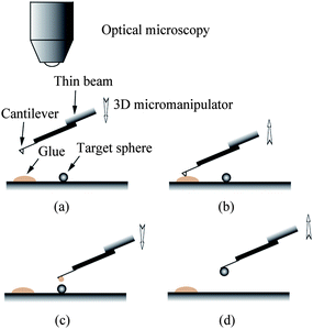 | ||
| Fig. 8 Procedure of gluing glass spheres at the end of AFM cantilevers: locating the glue (a), picking glue (b), locating the target glass sphere (c), gluing sphere and picking the probe up (d). | ||
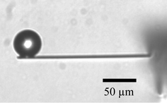 | ||
| Fig. 9 Optical microscopy image of the side view of a probe obtained by gluing a glass sphere at the end of a rectangular cantilever with a tip. | ||
The diameter of the spheres in the studies reported by Bhushan et al.15 and Wang et al.114 is larger than that of earlier experiments.36,16,17 There are several advantages to using large spheres. First, on rough surfaces, the hard contact positions between the sphere and sample surface are geometrically determined by the relationship between the distribution of asperities on the sample surface and the curvature of the sphere. Compared with small spheres, large spheres have relatively flat curvature and can therefore cover a larger area when in contact with the sample surface and the interaction occurs over a large area. Therefore, large spheres allow averaging of the hydrodynamic interaction on rough surfaces, otherwise one should make a statistical measurement on different positions on the sample. Spheres with radii from 10 μm to 12 μm have been used to measure slip length with AFMs.36,16,17 However, in the experiments reported here, the roughness values were relatively low, less than about 12 nm RMS (root mean square). When it comes to superhydrophobic surfaces, there is an inherently high roughness, and spheres with larger radii are desirable. Second, from eqn (3), one can see that the force exerted on the sphere increases with the square of the radius of a sphere as R2. Therefore, larger spheres are expected to increase the useful signal during experiments and improve the signal-to-noise ratio. Finally, the use of a large sphere minimizes Stokes friction force by increasing the cantilever distance from the sample surfaces. The Stokes friction force is the force generated by the body of the cantilever when the liquid is squeezed between the cantilever and the sample surface and was calculated by Vinogradova (2003) using a lubrication approximation, as
 | (13) |
 | (14) |
The smooth epoxy substrates were placed in a vacuum chamber at 30 mTorr (4 kPa pressure), 2 cm above a heating plate loaded with 500 μg of n-hexatriacontane and 2000 μg of Lotus wax. The n-hexatriacontane and Lotus wax were evaporated by heating them up to 120 °C. After coating, the specimens with n-hexatriacontane were placed in a desiccator at room temperature for three days for crystallization of the alkanes to generate the platelet nanostructure.13 After that, the specimen was heated in an oven (85 °C, 3 min.) and then immediately cooled down (5 °C) to interrupt the re-crystallization process to generate the hydrophobic surface. A contact angle of 91 ± 2.0° was measured on the hydrophobic surface. The specimens with Lotus wax were stored for seven days at 50 °C in a crystallization chamber and exposed to a solvent (20 mL of ethanol) in the vapor phase. A tubule nanostructure was produced on the specimen surface.56 The specimens with Lotus wax had contact angles of 167 ± 0.7°.
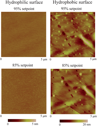
After fabrication, the hydrophilic, hydrophobic, and superhydrophobic surfaces were scanned in air with TMAFM over 5 μm × 5 μm scan area at the setpoint of 95%, as shown in Fig. 10. The RMS roughness of the hydrophilic, hydrophobic, and superhydrophobic surfaces is 0.2 nm, 11 nm and 178 nm, respectively, as shown in Table 2.
| Surfaces | RMS/nm | Peak-to-mean distance/nm | Contact angle (deg) | Slip length with contact mode AFM/nm | Slip length with TMAFM/nm |
|---|---|---|---|---|---|
| Hydrophilic | 0.20 ± 0.01 | 0.40 ± 0.01 | ∼0 | ∼0 | ∼0 |
| Hydrophobic surface | 11.0 ± 0.3 | 34 ± 1 | 91 ± 2.0 | 44 ± 10 | 43 ± 10 |
| Superhydrophobic surface | 178 ± 5 | 185 ± 5 | 167 ± 0.7 | 257 ± 22 | 236 ± 18 |
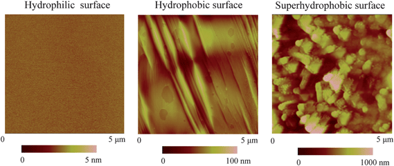 | ||
| Fig. 10 AFM images of hydrophilic, hydrophobic, and superhydrophobic surfaces in air.114,15 | ||
3.2 Contact mode AFM measurement
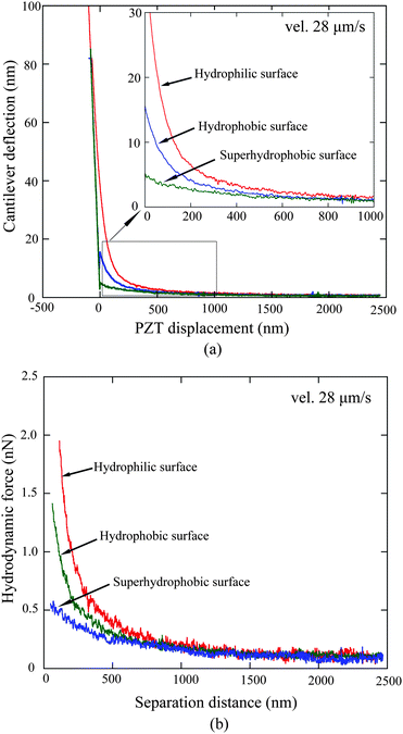
In this section, boundary slip measurement on the hydrophilic surface will first be discussed,68 followed by the measurement of boundary slip on hydrophobic and superhydrophobic surfaces.114In contact mode AFM experiments, the sample surfaces were driven relative to the sphere by a PZT (piezotube) with a constant velocity (28 μm s−1 for slip length measurement and 56 μm s−1 for the velocity dependence study of slip length, respectively). Low velocities of 0.4 μm s−1 and 0.8 μm s−1 were used to determine the electrostatic component. The cantilever deflection signal induced by hydrodynamic force and PZT displacement were obtained simultaneously, and this data was used for the calculation of hydrodynamic force which then was used to calculate slip length.
3.2.1.1 Elimination of electrostatic forces. In order to determine the electrostatic force for the hydrophilic surface shown in Fig. 10, two very low approach velocities, 0.4 and 0.8 μm s−1, were first applied to minimize the hydrodynamic force so that the force measured is dominated by the electrostatic force.114,68 The obtained cantilever deflection signal as a function of piezotube (PZT) displacement can be directly obtained. Then the deflection signal is added to the PZT displacement signal to get the actual separation distance between the sphere and the hydrophilic surface. After that, the cantilever deflection signal as a function of separation distance is obtained, as shown in Fig. 11. From the inset graph of Fig. 11 one can see that the deflection signal obtained at 0.8 μm s−1 is slightly larger than that obtained at 0.4 μm s−1 due to the hydrodynamic forces. The total deflection signal, hydrodynamic components obtained at velocities of 0.4 μm s−1 and 0.8 μm s−1, are taken as S1 and S2, and Shydro_1 and Shydro_2, respectively. By applying eqn (6), (7), and (8), the electrostatic double layer component is then obtained with the relationship of Selec = 2S1−S2, as shown in the inset of the Fig. 11. To verify the data processing, the hydrodynamic components for each velocity were then obtained with eqn (6) and (7). Because the velocities are very low, the hydrodynamic forces for 0.4 and 0.8 μm s−1 are very small compared with the electrostatic component, which means the measured deflection signal is dominated by electrostatic double-layer force when approach velocity is low. Moreover, the hydrodynamic component for the velocity 0.8 μm s−1 is approximately two times the velocity 0.4 μm s−1. The obtained electrostatic component was then subtracted from the total deflection signal obtained at higher approach velocities of 28 μm s−1 and 56 μm s−1 to determine the hydrodynamic components.
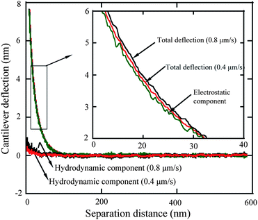 | ||
| Fig. 11 The measured cantilever deflection signal as a function of separation distance at approach velocities of 0.4 and 0.8 μm s−1, calculated electrostatic double-layer component, and pure hydrodynamic components. The pure hydrodynamic components for 0.4 and 0.8 μm s−1, and electrostatic component is obtained with eqn (6) to (8).68 | ||
3.2.1.2 Determination of hydrodynamic components and actual approach velocity. Once the electrostatic force is determined, approach velocities of 28 and 56 μm s−1 are applied to study boundary slip on the mica surface.114,68 The deflection signal as a function of separation distance for both approach and retract movement for approach velocities of 28 and 56 μm s−1 is shown in Fig. 12a and b. The time derivation of the actual separation distance between the sphere and the solid surface is taken as the actual approach velocity, as shown in the inset figures in Fig. 12. To obtain the actual deflection component generated by hydrodynamic force, the obtained electrostatic component is then subtracted from the total deflection signal. One can see the apparent increase of deflection signal from velocities of 28 to 56 μm s−1.
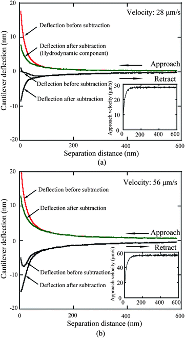 | ||
| Fig. 12 The measured cantilever deflection signal as a function of separation distance of both approach and retract movement at approach velocities of (a) 28 and (b) 56 μm s−1, and corresponding signals after the electrostatic double-layer components are subtracted. The insets show the actual approach velocity obtained from the time derivative of the actual sphere–mica surface separation distance.68 | ||
In addition to electrostatic force, the deflection component of Stokes friction force which is generated by the body of the cantilever beam when squeezing liquid needs to be considered. As shown in Fig. 12a and b, the gap of the cantilever deflection signal between approach and retract movement at the large separation distance increases as well because of the increasing Stokes friction. As stated earlier a large sphere was used in order to minimize the contribution of the cantilever beam to the liquid squeezing force. The cantilever deflection signal measured at a position far from the sample surface, where the deflection signal is independent of PZT displacement, is taken as the Stokes friction component and is subtracted from the deflection signal shown in Fig. 12.
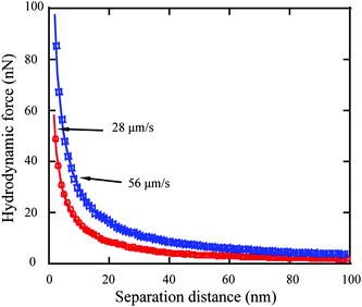
3.2.1.3 No-slip boundary condition on hydrophilic surface. After the electrostatic double-layer and Stokes friction components are subtracted from the cantilever deflection signal, the deflection signal solely generated by hydrodynamic force between the sphere and solid surface is obtained for both approach velocities of 28 and 56 μm s−1 by multiplying the deflection signal by the cantilever stiffness. Since both the sample surface and glass sphere are hydrophilic, eqn (3) and (5) are used to fit the obtained hydrodynamic force to obtain the slip length value for approach velocities of 28 and 56 μm s−1, as shown in Fig. 13. Slip lengths of 1.6 ± 1.5 and 0.7 ± 1.0 nm are obtained for approach velocities of 28 and 56 μm s−1, respectively. The small values are consistent and close to the derivation, which implies a no-slip boundary condition at the hydrophilic surface.68
 | ||
| Fig. 13 Hydrodynamic force as a function of separation distance at approach velocities of 28 and 56 μm s−1 and corresponding fitting curves (solid). | ||
3.2.2.1 Hydrodynamic force measurement and roughness treatment. By conducting the liquid drainage experiment on the hydrophobic and superhydrophobic surfaces at a velocity of 28 μm s−1, cantilever deflection as a function of PZT vertical displacement on hydrophobic and superhydrophobic surfaces was obtained, as shown in Fig. 14a.114 The data on the hydrophilic surface is shown for comparison. The obtained cantilever deflection signal is then processed as mentioned in Section 3.2.1, and the hydrodynamic force as a function of separation distance obtained after processing is shown in Fig. 14b. The hydrodynamic force gradually increases with decreasing separation distance for each surface. More importantly, one can see an apparent decrease of the hydrodynamic force as a sequence of hydrophilic, hydrophobic, and superhydrophobic surfaces.
 | ||
| Fig. 14 Comparison of (a) measured cantilever deflection versus PZT displacement and (b) calculated hydrodynamic forces as a function of separation distance on the hydrophilic, hydrophobic, and superhydrophobic surfaces with approach velocity of 28 μm s−1.114 | ||
Regarding hydrophobic and superhydrophobic surfaces, corresponding treatments were carried out before fitting the data to eliminate the influence of surface topography. As shown in Fig. 10, the hydrophobic and superhydrophobic sample surfaces are rough. Unlike the mica surface, the water among asperity structures on these surfaces will reduce the hydrodynamic force when the sphere contacts the surfaces. Therefore, surface roughness must be taken into consideration when conducting liquid drainage experiments on a rough surface with AFM. In other words, the position at which the sphere contacts the surfaces cannot be taken as a solid–liquid interface. Wang et al.114 took the mean surface as a virtual plane where the solid–liquid interface is located, called the virtual solid–liquid interface. The average peak-to-mean distance for each scan line of the whole area is taken as the distance offset between the actual contact position and virtual solid–liquid interface. For the hydrophobic and superhydrophobic surfaces, 34 nm and 185 nm offset to the separation distance are separately obtained by calculation.
3.2.2.2 Slip length calculation and approach velocity impact. After subtracting the electrostatic double layer force and Stokes friction force, and adding the relevant offset value to the corresponding separation distances, the measured hydrodynamic force data on hydrophobic and superhydrophobic surfaces are fitted with eqn (3) and (4) under the assumption that there is no slip on the sphere surface and boundary slip exists on the sample surfaces. The fitted curves are plotted in Fig. 15a and b with solid curves for hydrophobic and superhydrophobic surfaces at the approach velocity of 28 μm s−1, respectively. Slip lengths of 44 ± 10 nm and 257 ± 22 nm are obtained on hydrophobic and superhydrophobic surfaces, respectively, which implies the boundary slip increases with increasing hydrophobicity of solid surfaces.
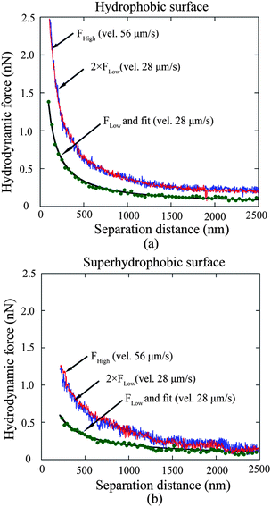 | ||
| Fig. 15 Hydrodynamic force at the approach velocity of 28 μm s−1 as a function of separation distance, and corresponding fitted curves on the hydrophobic (a) and superhydrophobic (b) surfaces. Experiments were also performed at the velocity 56 μm s−1 to explore velocity impact on boundary slip. Two times hydrodynamic force with approach velocity 28 μm s−1 is plotted to compare with that obtained with approach velocity 56 μm s−1 for each surface. Two curves agree with each other, which demonstrates the velocity independence of slip length measurement on both the hydrophobic and superhydrophobic surfaces in the study.114 | ||
Moreover, to explore the velocity dependence of slip length in liquid drainage experiments, a high approach velocity of 56 μm s−1 was applied to both hydrophobic and superhydrophobic surfaces, as shown in Fig. 15a and b, respectively. FLow and FHigh represent the hydrodynamic forces obtained with approach velocities of 28 μm s−1 and 56 μm s−1 for each surface. For each surface of approach velocity of 28 μm s−1, force versus distance was replotted using two times Flow in order to compare data at Fhigh. The two curves agree with each other well for each surface, which implies slip length is independent of approach velocity in a liquid drainage experiment with AFM, at least with an approach velocity up to 56 μm s−1.114
3.3 Tapping mode AFM measurement
In TMAFM experiments, the sample surfaces were driven at a very low velocity.15 The oscillation amplitude and phase signal were used to obtain the damping coefficient for slip length measurement, and the deflection signal was monitored as an indicator to determine hard contact position. The diameter of the sphere glued at the end of the cantilever used in TMAFM method was 42.4 ± 0.8 μm, and the stiffness of the cantilever was calibrated as 1.5 ± 0.1 N/m.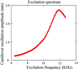 | ||
| Fig. 16 Excitation spectra and corresponding fitting of AFM cantilever oscillation as a function of excitation frequency in water. By fitting, a quality factor of 5.2 and resonance frequency of 11.7 kHz are obtained.15 | ||
The amplitude and phase shift data as functions of piezo displacement during the cantilever approach to the hydrophilic, hydrophobic, and superhydrophobic surfaces were obtained as shown in Fig. 17. Both oscillation amplitude and phase shift decrease with decreasing piezo displacement, which implies increasing hydrodynamic damping coefficient. Additionally, the amplitude drops more rapidly on the hydrophilic surface than the other two surfaces, indicating a bigger hydrodynamic damping coefficient on the hydrophilic surface. Unlike in contact mode AFM measurements where the deflection signal gradually increases with decreasing piezo displacement, the deflection signal remains around zero until contact with the sample surface. Therefore, in the tapping mode AFM method the contact position can be obtained directly from the DC-deflection in contrast to the contact mode AFM method where one has to extrapolate the linear part of the deflection to zero to get the contact position. The position at which the deflection signal turns to increase can be taken as the zero separation position. Because the deflection signal remains constant (zero) until the tip contacts the sample surface, a piezo displacement larger than zero can be directly taken as the separation distance between the sphere and sample surfaces.
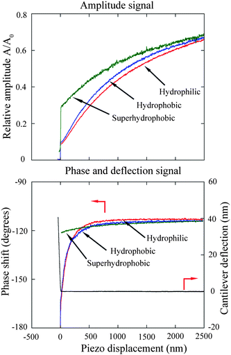 | ||
| Fig. 17 The measured relative amplitude, phase shift data, and deflection signal of the oscillating cantilever as functions of piezo displacement when the cantilever approaches the hydrophilic, hydrophobic, and superhydrophobic surfaces. The deflection signal is used to determine the actual contact position with a resolution of 1 nm.15 | ||
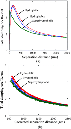 | ||
| Fig. 18 Total damping coefficient (a) as a function of separation distance between the sphere and sample surfaces and corresponding fitting curves (b) on the hydrophilic, hydrophobic and superhydrophobic surfaces. The separation distances are corrected by adding the offset distances for the hydrophobic and superhydrophobic surfaces due to high value of roughness in fitting curves (b). The hydrophilic surface has highest value of hydrodynamic damping coefficient, which implies lowest degree of boundary slip of three surfaces.15 | ||
As indicated in contact mode AFM method, the measured separation distance needs to be corrected for roughness effects. Distance offsets are added to the separation distances for the hydrophobic and superhydrophobic surfaces before these data are fitted. The average peak-to-mean distances, 34 and 185 nm for the hydrophobic and superhydrophobic surfaces, respectively, are taken as the distance offset between the measured contact position and the virtual solid–liquid interface. Then the distance offsets are added to the separation distance for fitting the data on the hydrophobic and superhydrophobic surfaces.
To quantitatively evaluate the degree of boundary slip at the solid–liquid interfaces of the three surfaces, the calculated hydrodynamic damping coefficients were separately fitted. For the hydrophilic surface, the damping coefficient was fitted with eqn (9) taking the factor f* = 1 with the assumption that no boundary slip exists at the hydrophilic surface, while the damping coefficients on the hydrophobic and superhydrophobic surfaces are fitted with eqn (4) and (9). After adding the offset values of 34 and 185 nm to the separation distance, the total damping coefficient as a function of corrected separation distance (distance + offset) are shown in Fig. 18b. Corresponding fitting curves are also shown here. Slip lengths of 43 ± 10 nm and 236 ± 18 nm are obtained on the hydrophobic and superhydrophobic surfaces, respectively. It is well known that air may be trapped in groove structures on rough hydrophobic surfaces.79 Bormashenko et al.20 reported a phenomenon of vibration-induced Cassie–Wenzel wetting transition (destruction of air pockets) by vibrating droplets on micro-patterned polystyrene surfaces. In the experiment, the pressure induced by the oscillating sphere is expected to be smaller than those reported by Bormashenko et al.20 to generate the Cassie–Wenzel transition.
Table 2 summarizes the surface properties and slip length values obtained with both contact mode AFM and TMAFM methods. The slip lengths obtained using both methods are close to each other for hydrophobic and superhydrophobic surfaces. The slip length value obtained for the rough hydrophobic surface is close to the value obtained on smooth hydrophobic surfaces using the PIV method.59 On superhydrophobic surfaces some authors reported a slip length ranging from 100 nm to several microns, depending on the patterns, using μ-PIV and AFM54 or a commercial rheometer.31
3.4 Role of nanobubbles on boundary slip
As stated in the Introduction, nanobubbles are generally thought to be the reason for boundary slip at the solid–liquid interface. In this section, nanobubble imaging and boundary slip studies will be correlated to explore the role of nanobubbles on boundary slip.114To check whether nanobubbles are present on the surfaces, the three surfaces were imaged with TMAFM in DI water.114 A featureless image was obtained on the mica surface with 95% setpoint of cantilever free oscillation, as shown in Fig. 19 (left). Then, a higher load (85% setpoint) was applied to image the surface. No change was observed. However, for the hydrophobic surface, spherical objects were observed over the whole area, as shown in Fig. 19 (right). The diameter and height of the objects are about 150 nm and 6 nm, respectively. To verify that the objects are nanobubbles, 85% setpoint of free oscillation amplitude was then applied. Similar to the experiment performed by Bhushan et al.,12 bigger nanobubbles with less density over the surface were observed at a lower setpoint. Here one can see that although the hydrophobic surface is rough, one can distinguish nanobubbles from the roughness. However, on the superhydrophobic surface, nanobubble images were not obtained due to the high value of roughness.
 | ||
| Fig. 19 AFM images of hydrophilic and hydrophobic surfaces in DI water with 95% and 85% setpoint of free amplitude, corresponding to about 0.09 nN and 0.26 nN normal forces, respectively. Nanobubbles with a typical diameter of 150 nm are observed on the hydrophobic surface. No change is observed on hydrophilic surface between high and low load scanning. However, nanobubble coalescence is observed on the hydrophobic surface after high load scanning.114 | ||
Tretheway and Meinhart105 calculated the slip length for fluid flow between two infinite parallel plates by modeling the presence of either a depleted water layer or nanobubbles as an effective air gap at the wall. They reported that the slip length increases with an increasing value of air gap thickness, assuming that air covers the wall continuously. For an intermittent surface coverage of nanobubbles, the slip length increases with increasing nanobubble height and surface fraction covered by nanobubbles. A schematic of the role of nanobubbles on boundary slip in liquid drainage experiments is shown in Fig. 20, where hb is an effective thickness of the air gap induced by nanobubbles. When a gas layer exists between a solid surface and a liquid, the slip length generated by the discontinuity of viscosity at the liquid–gas interface is given as,111
 | (15) |
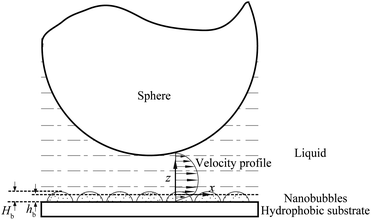 | ||
| Fig. 20 Schematic of a sphere–flat system with nanobubbles distributed on the flat surface. The presence of nanobubbles on the flat surface changes the velocity profile between the sphere and the plane surface, which results in an increase of slip length. The nanobubbles with a height Hb are approximated by a gas layer with effective thickness hb.114 | ||
The viscosity for water and air at a temperature of 300 K are about ηw = 851.5 μPa s and ηa = 18.6 μPa s, respectively.64 Thus, the obtained slip length b may be 45 times air gap thickness hb due to high value of ηw/ηa.
According to the theoretical analysis of eqn (15), an approximately 1.0 nm thick air gap hb is needed to generate a slip length of 44 nm (in contact mode AFM method) or 43 nm (in TMAFM method) on the hydrophobic surface. Because the nanobubbles are actually discretely distributed over the sample surface, but do not act as a continuous air gap, Wang et al.114 treated the effective air gap hb thickness as a function of nanobubble height Hb, given as
| hb = Hbϕ | (16) |
To summarize, theoretical analysis shows that nanobubbles favor boundary slip. The existence of nanobubbles on the hydrophobic surface is verified by conducting TMAFM in water. The increasing slip length from hydrophobic to superhydrophobic surfaces is expected to be because of increasing hydrophobicity.
3.5 Summary
Both contact mode AFM and TMAFM can be used to study boundary slip at solid–liquid interfaces through slip length measurement. In contact mode AFM method, the slip length is obtained by fitting the measured hydrodynamic force applied to a sphere as a function of separation distance between the sphere and solid surfaces when two surfaces approach each other. In data processing, the cantilever deflection impact on the actual separation distance and approach velocity, as well as the impact of the electrostatic double-layer force between the sphere and solid surfaces and Stokes friction force on cantilever deflection, need to be eliminated. Cantilever deflection signal is added to the measured PZT displacement to obtain the actual separation distance. The actual approach velocity is then obtained through time derivation of the actual separation distance. Electrostatic force can be determined by performing a liquid drainage experiment with two low velocities in order to minimize the hydrodynamic force so that the force measured is dominated by the electrostatic force. The cantilever deflection signal measured at a position far from the sample surface, where the deflection signal is independent of PZT displacement, is taken as the Stokes friction component. In the tapping mode AFM method, the amplitude and phase shift data of an oscillating sphere are recorded during approach to sample surfaces at low velocities. These data are then used to get the hydrodynamic damping coefficient to obtain the slip length.No-slip boundary condition on hydrophilic surfaces was obtained by performing liquid drainage experiments using contact mode AFM method. For hydrophobic and superhydrophobic surfaces, experimental results show velocity independence of boundary slip by performing the drainage experiment with different approach velocities. To separate influences of surface roughness and hydrophobicity on boundary slip for hydrophobic and superhydrophobic surfaces, the average of peak-to-mean distance for each surface can be added to the separation distance as an offset to compensate for roughness influence on the measurement. Slip lengths of 44 and 257 nm were obtained with contact mode AFM method for hydrophobic and superhydrophobic surfaces, respectively, which are close to the values of 43 and 236 nm obtained with TMAFM. The experimental results on surfaces with different hydrophobicities demonstrate increasing boundary slip with hydrophobicity of sample surface.
As a possible reason for boundary slip, nanobubbles can be correlated with boundary slip. By imaging nanobubbles on the hydrophobic surfaces, the measured slip length on the surface can be explained by approximately treating the intermittent nanobubbles as a continuous gas layer with an efficient thickness, which provides an approach to reveal the influence of nanobubbles on boundary slip.
4. Nanobubbles on hydrophobic surfaces
In this section, properties of nanobubbles on hydrophobic surfaces will be studied. Interaction of nanobubbles with the substrates supporting them may affect nanobubble immobility, which is of importance. To study the mechanical properties of nanobubbles and solid–liquid interactions on the nanoscale, tip–nanobubble interactions need to be investigated. Various studies including nanobubble imaging,12 nanobubble–substrate interaction,116 tip–nanobubble interaction,12,115 and nanobubble immobility115 will be discussed in this section.4.1 Experimental
Like in the boundary slip study, a modified tip holder was used to study nanobubbles.12,115,116 A silicon cantilever rotated force-modulation etched silicon probe (RFESP) (Digital Instruments) with a tip radius < 10 nm and a stiffness of 3 N/m quoted by the manufacturer was used. The measured resonance frequencies in air and water were about 73 and 26 kHz, respectively. While imaging in air and liquid, the cantilever is vibrated at the resonance frequency.A polystyrene (PS) surface for nanobubble imaging used in the study was prepared by the spin coating method on a silicon (100) wafer. The polystyrene particles (molecular weight 350![[thin space (1/6-em)]](https://www.rsc.org/images/entities/char_2009.gif) 000, Sigma-Aldrich) were dissolved in toluene (Mallinckrodt Chemical) with different concentrations to control the thickness of films, and the speed for spin coating was 500 rpm. The contact angle of the PS surface obtained with the sessile drop method was 95 ± 3° degrees for continuously coated PS films, which shows that the sample surface is hydrophobic.
000, Sigma-Aldrich) were dissolved in toluene (Mallinckrodt Chemical) with different concentrations to control the thickness of films, and the speed for spin coating was 500 rpm. The contact angle of the PS surface obtained with the sessile drop method was 95 ± 3° degrees for continuously coated PS films, which shows that the sample surface is hydrophobic.
All experiments were performed in deionized (DI) water. The sample surfaces were first imaged in air by TMAFM. Then the samples were immersed into DI water to perform liquid imaging. The free oscillation amplitude of the cantilever at working frequency was about 7.0 nm. An amplitude of 6.65 nm (namely 95% of free amplitude) was chosen for nanobubble imaging. In the study of nanobubble coalescence and movement, an amplitude of 6.30 nm (90% of free amplitude) was chosen to apply higher load.12 To compare the consequences of nanobubble coalescence and movement, a central 2 μm × 2 μm scan area was generally selected to perform higher load scans. Then imaging was carried out in a 5 μm × 5 μm scan area with a 95% setpoint to check corresponding changes. The choice of the 95% setpoint is important to avoid any unexpected change to nanobubbles.
In the study of nanobubble–substrate interaction,116 a PS film with a thickness of 2.8 ± 0.3 nm was used. After spin-coating, the PS samples were put into an oven at 45 ± 3 °C for about 4 h to remove the remaining toluene. The sample was first imaged in air using TMAFM and then immersed into DI water for time-series imaging.
In the study of tip–nanobubble interaction, a so-called auto ramp function combined with force modulation mode was used in TMAFM to get a series of amplitude and phase shift as a function of distance curves over a certain area in the liquid.12 In auto ramp function, the piezotube performs a vertical extending and retracting movement relative to the tapping cantilever tip along the x and y axes separately with a fixed step, and the cantilever driving frequency and amplitude remains constant. Piezotube vertical frequency was chosen as 1 Hz, and vertical extension was 200 nm during auto ramping. A step of 30 nm was chosen along both x and y axes on an approximate 1 μm × 1 μm scan area which contained a nanobubble. At each test location on the nanobubble, amplitude and phase as a function of distance curves were obtained. In the contact mode AFM study of tip–nanobubble interaction, the force distance curves were measured.
In the study of nanobubble immobility, the continuously and partially coated PS films were prepared by spin-coating a PS solution with concentrations of 0.20% (weight) and 0.04% (weight) in toluene (Mallinckrodt Chemical), respectively, onto silicon substrates.115 When spin coating the PS solution onto the silicon wafer, the spin-coated PS films will change from partially coated to continuously coated with increasing PS concentration.96 After imaging in air, the samples were first imaged with TMAFM in DI water after immersion in DI water for about 220 min to allow sufficient time for nanoindent formation.116 The amplitude setpoints were applied with a sequence of 95%, 80%, 95%, 60%, and 95% in order to study the effect of load on the mobility of the nanobubbles. There was a total of three 95% setpoint images. The first scan was used to check the initial stage of the nanobubbles, and the two later scans were used to check the status of the nanobubbles after high load imaging of 80% and 60% setpoint, respectively. The two high loads of amplitude setpoint were used to evaluate nanobubble immobility on each surface. After liquid experiments, the sample surfaces were imaged with TMAFM in air to check surface topography changes before and after adding water.
4.2 Nanobubble imaging
By performing TMAFM in air, a featureless image of the original PS coated silicon wafer surface was obtained, as shown in Fig. 21a. The RMS roughness and peak to valley distance Rmax are 0.21 nm and 2.3 nm, respectively. Fig. 21b shows the image of the PS surface immersed in DI water. The entire surface is covered with spherical cap like domains. The diameter and height of these caps are generally on the order of 200 nm and 20 nm, respectively. The RMS roughness and Rmax are 8.2 nm and 68.7 nm, respectively, which are about two orders of magnitude larger than that obtained in air. Some big domains are observed in the vicinity where nanobubble density is lower than other places. That may be because of local nanobubble coalescence.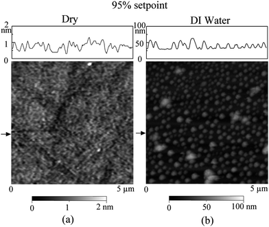 | ||
| Fig. 21 Comparison of images of PS coated silicon wafer using tapping mode AFM in (a) air and (b) DI water. Section profiles are taken at locations shown by arrows in AFM images.12 | ||
Fig. 22a (left) was obtained at 95% setpoint and full 5 μm × 5 μm area scan. Then the central 2 μm × 2 μm area scan was performed two times with the same 95% amplitude setpoint. After that, the 5 μm × 5 μm area was imaged again with 95% setpoint to get the image shown in Fig. 22a (right). One can find bigger nanobubbles generated in the central area with lower density. The diameter and height of the nanobubbles increase to 420 nm and 55 nm from 200 nm 20 nm, respectively, in Fig. 22a. Therefore, some nanobubbles must coalesce and generate bigger ones. The only difference between the 2 μm × 2 μm central area scan of Fig. 22a (right) and Fig. 22a (left) is the scan speed. When working at the same scan rate, the scan speed in the 5 μm × 5 μm area scan is one-and-a-half times higher than that in the 2 μm × 2 μm area scan. Assuming the power transferred from cantilever tip to sample surfaces is constant during the certain period of time, the low scan speed implies higher power transfer at the same scan area than at high scan speed, and nanobubbles suffer more disturbance. Therefore, the coalescence occurred even with the same setpoint of amplitude.
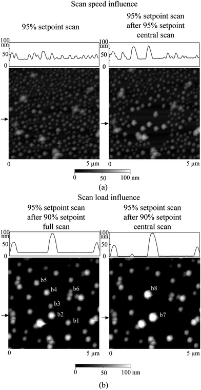 | ||
| Fig. 22 Sequence of nanobubble images obtained in the same 5 μm × 5 μm scan area with (a) 95% amplitude setpoint scan (left); 95% amplitude setpoint scan preceded by scanning with 95% amplitude setpoint in central 2 μm × 2 μm area for two times (right). Nanobubble coalescence is observed with lower scan speed in the central area. (b) 95% amplitude setpoint scan preceded by scanning with 90% amplitude setpoint in full 5 μm × 5 μm scan area (left); and 95% amplitude setpoint scan preceded by scanning with 90% amplitude setpoint in central 2 μm × 2 μm area for two times (right). Further coalescence of nanobubbles is observed. Section profiles are taken at locations shown by arrows in AFM images.12 | ||
From the above experiment, one can find that nanobubbles are very sensitive to scan parameters while imaging. In addition to scan load, scan speed can also affect nanobubble imaging. To get original nanobubble images without movement and coalescence, a higher setpoint (corresponding to lower scan load), higher scan rate, and larger scan area are desirable.12 If the scan parameters are not chosen properly, the nanobubbles will be coalesced or moved during imaging, and in some cases cannot be observed.
After applying 90% setpoint scan to the whole 5 μm × 5 μm area of Fig. 22a (right), a 95% setpoint scan was performed in the full area, and nanobubble images with a lower density were obtained, as shown in Fig. 22b (left). Nanobubble density is reduced while the nanobubble size abruptly increases with the normal diameter over 550 nm and height over 77 nm. With lower nanobubble density, it is possible to track certain nanobubbles' coalescence. In the central area containing six numbered nanobubbles of Fig. 22b (left), central 2 μm × 2 μm area scan was performed two times with 90% setpoint. After that, 95% setpoint scan was performed over the full area, and a further nanobubble coalescence image was obtained, as shown in Fig. 22b (right), where the diameter and height of nanobubbles increase from 550 nm, 77 nm up to 690 nm and 100, respectively.
By comparing Fig. 22b (left) with (right), one can find that, except for the six numbered nanobubbles in the left, the sizes and locations of other nanobubbles remained unchanged in Fig. 22b (right). Based on their locations, nanobubbles b1, b2, and b3 were believed to coalesce and generate the bigger nanobubble b7. Similarly, b4, b5, and b6 joined together and generated nanobubble b8. More importantly, one can find that during nanobubble coalescence, small nanobubbles (b1, b3 and b5, b6) tend to move first and coalesce with b2 and b4, generating bigger nanobubbles. This should be because the big nanobubbles have a strong interaction with the surface due to their long length of contact line with the surface.
To verify nanobubble coalescence, the quantity of gas molecules trapped in nanobubbles before and after coalescence was calculated. Bhushan et al.12 assumed the total number of gas molecules trapped in nanobubbles before and after coalescence kept constant. According to the Laplace–Young equation:5,6,49
| Δp = 2γ/R | (17) |
| Nanobubble | Height Hi/nm | Radius Ri/nm | Pressure pi (atm) | Volume Vi (×106nm3) | p i × Vi (×10−6 nNm) |
|---|---|---|---|---|---|
| b1 | 51.8 | 325.6 | 5.4 | 2.6 | 1.4 |
| b2 | 78.2 | 490.9 | 3.9 | 8.9 | 3.5 |
| b3 | 61.1 | 364.7 | 4.0 | 4.0 | 2.0 |
| b7 | 99.7 | 550.3 | 3.6 | 16.2 | 5.9 |
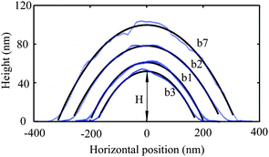 | ||
| Fig. 23 Cross section profiles of nanobubble b1, b2, b3 and b7 in Fig. 22b through the apex of nanobubbles, and the solid curves correspond to least-square fit curves by fitting the profiles as circular arcs. H is the height of nanobubbles shown in Table 3.12 | ||
The result shows that pb7 × Vb7 = 5.9 × 10⁻⁶ nNm, which is smaller than pb1 × Vb1 + pb2 × Vb2 + pb3 × Vb3 = 6.9 × 10⁻⁶ nNm of nanobubbles b1, b2, and b3. Note here a difference of 14.5% of the quantity pi × Vi before and after coalescence. This occurs because of uncertainties in the value of the measured volume and also to the gas dissolution during nanobubble movement and coalescence. Since nanobubbles are highly deformable and easily penetrated during imaging, the height of nanobubbles during imaging should be underestimated.110,28,123 According to the Laplace–Young equation, the pressure in big nanobubbles is smaller than that in small ones. The influence of height underestimation should be larger for big nanobubbles than small ones for their much softer properties. In summary, there should be less than 14.5% of the gas dissolved into water during this process.
4.3 Nanobubble–substrate interaction
Although nanobubbles show potential applications in micro/nanofluidics, little is known about the physical interaction of nanobubbles with the substrate supporting them, which are both fundamentally interesting and practically important. Physical interaction of nanobubbles with ultrathin polymer films in the presence of nanobubbles has seldom been done. Recently, a phenomenon of nanobubble induced nanoindents on ultrathin PS films in DI water has been reported by Wang et al.116 A time-series imaging was performed to study the evolution of nanoindents on PS surface in water. A strong correlation between the changes in surface morphology of PS surface and the presence of nanobubbles was observed and discussed by considering the interaction between the nanobubbles and the PS surface. Various factors that could influence the structure of PS surface, such as film thickness and nanobubble size, was discussed.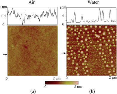 | ||
| Fig. 24 Comparison of images of PS coated silicon wafer using tapping mode AFM in (a) air and (b) DI water. Two groups of size of nanobubbles can be observed. The section profiles are taken at positions shown by arrows in AFM images and show structures of sample surface and nanobubbles.116 | ||
Time-series images of the PS sample immersed in water for a duration of several hours are shown in Fig. 25. The section profiles are taken at positions shown by arrows in AFM images. It is clear that the morphologies of the nanobubbles and the PS surface experienced continuous change with time.116 At the time of 10 min, spherical nanobubbles with smooth profiles are observed, which can be seen through the section profile of Fig. 25a. After 40 min, both small nanobubbles and large nanobubbles appear to shrink in size. Most distinctively, circular rims emerged at the perimeter of large nanobubbles, which also can be seen from the section profile (Fig. 25b). Typical height of the rims is about 1.0 nm. After 150 min, the typical height of rims increased to about 2.0 nm (Fig. 25c). Most of the small nanobubbles have disappeared in Fig. 25c, leaving small nanoindents at their original positions with a diameter of about 20 nm. One nanoindent is pointed out by an arrow in Fig. 25c for example. After 225 min, another scan area was chosen to exclude the possibility of cantilever tip influence on the evolution of nanobubbles and formation of nanoindents. All the small nanobubbles disappeared and left densely distributed nanoindents. However, bigger nanobubbles were still on the surface. The presence and evolution of nanobubbles can also be observed through phase images. The phase shift data is important to reveal mechanical properties in TMAFM.8 Using phase shift data, Bhushan et al.12 studied the viscoelastic properties of cantilever-tip interaction. Here, phase shift images are shown to help us distinguish surface features on the PS surface. In Fig. 25, the black circular objects in phase shift images represent the existence of nanobubbles. The phase images reveal that the density of small nanobubbles gradually reduced with time and finally disappeared at 225 min. 3D images for a certain nanobubble circled in Fig. 25a and c after 10 min and 150 min was given in Fig. 26a and b to illustrate the topography change. At the time of 10 min, the nanobubble has a smooth profile. However, a rim appeared around the nanobubble at the time of 150 min. The diameter of the nanobubble lightly shrinks after appearance of the rim.
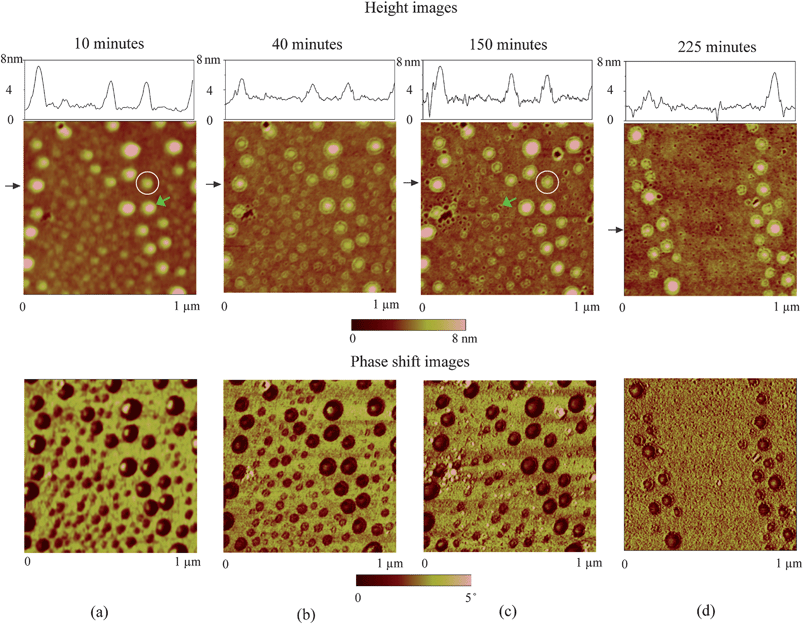 | ||
| Fig. 25 Sequence of nanobubble height images and phase shift images as a function of time immersed in DI water in 1 μm× 1 μm scan area: (a) 10 min; (b) 40 min; (c) 150 min; and (d) 225 min. Rims appear in (b). Small nanobubbles gradually disappear, leaving nanoindents at corresponding sites, one of which is pointed out by an arrow in (c) and finally small nanobubbles disappear in (d). The section profiles are taken at positions shown by arrows in AFM images. From section profiles, one can see that rims appear from 40 min and gradually grow up with immersion time. The nanobubble pointed out in (a) is used to calculated nanobubble inner pressure and the ones circled by white circles in the first and third images are used to show rim structures through 3D images.116 | ||
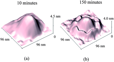 | ||
| Fig. 26 3D images of a nanobubble circled in Fig. 25a and 25c at 10 min (a) and 150 min (c) after the PS sample was immersed into DI water. The profile of the nanobubble is smooth at 10 min and a rim appeared around the nanobubble at 150 min.116 | ||
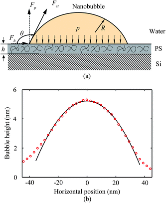 | ||
| Fig. 27 (a) Schematic of a nanobubble on the ultrathin PS film in water. The surface tension force Fst can be decomposed into perpendicular force Fp and horizontal force Fh. The inner pressure uniformly applies on the PS surface inside the nanobubble. (b) Cross section profile of a nanobubble marked by an arrow in Fig. 25a through apex of the nanobubble and corresponding least-square fit curves (solid) by fitting the profile as circular arcs.116 | ||
A nanobubble of moderate size is taken as an example as marked by an arrow in Fig. 25a. The cross section through the center of the nanobubble is fitted with a circular arc as shown in Fig. 27b, and the radius of the nanobubble is estimated to be 83.5 nm. The contact angle θ of water is derived to be about 162.5°, which is close to 168.4° reported by Simonson et al.95 for nanobubbles on a similar PS surface. The presence of the nanobubble clearly introduces two important factors to the PS film: the high inner pressure and surface tension force due to the three phase contact line, which increase the instability of PS film nearby nanobubbles.
4.3.2.1 Influence of inner pressure. According to the Laplace–Young eqn (17), for the nanobubble shown in Fig. 27b, the inner pressure is about 1.85 MPa, which is substantially larger than the ambient pressure (101 kPa). For nanobubbles with diameters smaller than 40 nm, the inner pressure should be even higher than that of the nanobubbles marked in Fig. 25. As illustrated in Fig. 27a, the large inner pressure would squeeze PS chains out of the nanobubble, contributing to the formation of rims around nanobubbles.
To demonstrate the contribution of inner pressure to the formation of rims and nanoindents, nanoindentation experiments using a silicon nitride AFM tip were carried out on a PS surface using a tip radius of about 50 nm. A normal load of 0.84 nN was continuously applied on the surface for about 30 min. After that, an apparent deformation was observed on the PS film. The mean contact pressure applied to the contact area is about 55.3 MPa based on Hertz analysis with the bulk value of elastic modulus of 3.2–3.4 GPa22 and Poisson's ratio of 0.32521 for PS. The actual value of elastic modulus for ultrathin PS film may be smaller than the bulk value, which would predict a lower Hertz stress. Thus, the data suggest that indentation of the PS film is possible with rather small loads.
Here, one should note that the thickness of PS film also contributes to the formation of rims and nanoindents. In the bulk state, polymer chains are entangled with each other, and the mobility of polymer chains is greatly impeded.94 Near the surface or interface, the degree of entanglement is greatly reduced, and the mobility of polymer chains is enhanced, leading to relatively weak interaction between PS chains. The polymer chain packing theory23 and dynamic molecular simulation,74 together with a recent experiment,94 reveal that the entanglement density in an ultrathin polymer surface is significantly reduced, which reduces the interaction between different chains. Hence, PS chains move towards the outside of the nanobubbles with high inner pressure p and perpendicular component Fp (to be described later) of surface tension force, resulting in the appearance of rims around nanobubbles.
4.3.2.2 Influence of three phase contact line. Based on the Wang et al.116 analysis, the total surface tension force Fst along the contact line can be decomposed into two sub-components: the perpendicular force Fp and the horizontal force Fh. Both Fp and Fh increase the instability of the PS films near the three phase contact line. The perpendicular component of surface tension force Fp works collaboratively with the inner pressure to pile up the PS chains at the perimeter of the nanobubble, contributing to the formation of rims as shown in the height images of Fig. 25. However, the horizontal component Fh is likely to stretch the PS film and lead to fracture.
The total horizontal force Fh acting along the three phase contact line is given as:
| Fh = Fstcos(180 − θ) = γ·πD·cos(180 − θ) | (18) |
| σ = Fh/(πD·h) = γ·cos(180 − θ)/h. | (19) |
If the horizontal component Fh is the main reason for the formation of nanoindents, there should be more nanoindents appearing around nanobubbles. From the height image of Fig. 25c, one can find that most nanoindents appear on the sites of small nanobubbles, and very few nanoindents appear around the bigger nanobubbles, which means it is high inner pressure p combining with perpendicular component Fp, but not Fh dominating the process of the generation of rims and nanoindents. This can also be observed through the structure of rims around bigger nanobubbles, as shown in section profiles of Fig. 25 and 3D image of Fig. 26b. After rims appear around the nanobubbles, the topography of PS film outside of rims remains flat. From the conservation of materials of PS chains, the appearance of rims should be mainly because of PS chain movement from inside to outside of nanobubbles due to high inner pressure.
Based on the experimental observation, a schematic diagram was given to demonstrate the detailed process of nanoindented surface formation and the influence of nanobubble size during this process, as shown in Fig. 28. At stage 1, different sizes of nanobubbles appear on the PS sample which is immersed into DI water for several minutes. Both nanobubbles and PS sample surface are not changed yet, corresponding to the image of Fig. 25a. At stage 2, the sample has stayed in DI water for several dozens of minutes. Because of the existence of inner Laplace pressure of nanobubbles and surface tension force along three phase contact line, the PS chains below the nanobubbles is under an imbalance condition, which leads to a fracture of the PS film. Rims appear around the nanobubbles. At the same time, the rims confine the nanobubbles and make them shrink. Stage 2 corresponds to the images of Fig. 25b and 25c, where round rims appear around the nanobubbles and gradually grow up, and parts of small nanobubbles begin to disappear. At stage 3 which corresponds to the image of Fig. 25d, the PS sample has been in DI water for over 200 min. The smaller nanobubbles have totally disappeared because the changed topography is no longer favorable for them.
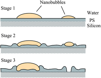 | ||
| Fig. 28 Schematic of the process for nanoindents formed on the PS surface. The whole process is divided into three stages. Stage 1: nanobubbles formation; Stage 2: Rims appear and nanobubbles shrink; and Stage 3: Rims grows around large nanobubbles and small nanobubbles disappear with appearance of nanoindents.116 | ||
It is clear that the size of nanobubbles is strongly correlated with the speed of nanobubble disappearance and nanoindent formation. Smaller nanobubbles have greater inner pressure. Therefore, the speed of topography change is expected to be faster than bigger ones. Additionally, smaller nanobubbles are much more sensitive to the change of topography. Once the nanoindents grow to a size comparable to the diameter of nanobubbles, small nanobubbles will disappear. However, bigger nanobubbles are not as sensitive as smaller ones to the topography change. As revealed through experimental observation, the rims around bigger nanobubbles gradually grow, and the nanobubbles continue to stay on the rims.
In summary, the presence of nanobubbles is crucial for the formation of nanoindents, and the size of nanobubbles can greatly influence the process. Based on this experiment, it is found that nanobubbles with diameters larger than 100 nm and smaller than 40 nm hinder the process. When the diameters of nanobubbles are larger than 100 nm, the inner pressure is low, and they cannot be dissolved easily during experiment. In contrast, when the diameters are smaller than 50 nm, the nanobubbles will dissolve quickly and leave smaller nanoindents sitting on the sites. Nanobubbles with a diameter of about 60–80 nm should be desirable for the process. In view of its ease of use, the phenomenon revealed in this paper could be applied to fabricate nanopattern structures on polystyrene surfaces. Additionally, this work should also provide instructive information for the application of polymer thin films in aqueous solutions.
4.4 AFM tip–nanobubble interactions
In order to show nanobubble mechanical properties and solid–liquid interaction on the micro/nanoscale, in this section, tip–nanobubble interaction study will be discussed. To study tip–nanobubble interactions, Bhushan et al.12 and Wang et al.115 applied force modulation curves in TMAFM and force distance curves in contact mode AFM.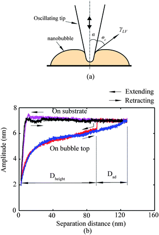 | ||
| Fig. 29 (a) Schematic of interaction between cantilever tip and nanobubble, and (b) amplitude signal as a function of separation distance during extending and retracting modes with a tapping cantilever tip on the PS substrate and a nanobubble top. The amplitude gradually decreases with decreasing separation distance for the nanobubble as compared with that on PS substrate.12 | ||
By performing force modulation experiments over a nanobubble, experimental results show a clear trend of variation for the value Dheight and Dad, as shown in Fig. 30b and c. Six curves are selected from the data taken at 16 points along a randomly selected scan line in the auto ramp function, as shown in Fig. 30a. The exact locations of these six curves are marked in Fig. 30b. For curve 1, one can expect that the tip is on the edge of the nanobubble. That is because the extending curve is just like that on the substrate while the retracting curve is typical of on-nanobubble response, similar to the retracting curve on nanobubble in Fig. 29b. From curve 2 to curve 5, the tip extends and retracts along the profile of the nanobubble until curve 6, where the tip interacts with the substrate, and on-nanobubble response is not observed. One should note that for all curves, the tip encountered hard contact with substrate surface at the same location where the amplitude drops down to a value close to zero. This can be used to distinguish nanobubbles from contamination particles during nanobubble imaging. According to the force modulation curve, Bhushan et al.12 believed that the cantilever tip penetrated the nanobubble, and the three phase contact line moves upward along the tip axis during the process of tip–nanobubble interaction in force modulation mode.
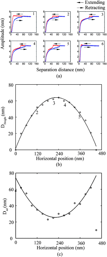 | ||
| Fig. 30 (a) Selected six curves (corresponding to points 1–6 in Fig. 30b) of amplitude as a function of separation distance along a scan line of a nanobubble. At locations 1 to 3, height of nanobubble increases and at locations 4–6, height of nanobubble decreases. (b) Height of nanobubble (Dheight) as a function of horizontal position along the scan line. The value first increases and then decreases following the profile of nanobubble. (c) The distance Dad with respect to each point of Fig. 30b. The value Dad decreases with increasing height of nanobubble (Dheight) along the scan line and vice versa.12 | ||
Two trends can be observed from the tip–nanobubble interaction curves. One is that Dheight first increases and then decreases following the profile of the nanobubble, as shown in Fig. 30b. The other observation is that the trend of Dad with horizontal position is inversely related with Dheight. It is clear that Dad reaches its minimum value around the apex of the nanobubble profile. At the edge of the nanobubble, Dad is large. The inverse relationship between Dad and Dheight is believed to be due to the variation of the length of the contact line between the cantilever tip and the nanobubble at the different position of the nanobubble. When the tip–nanobubble interaction occurs at the edge of the nanobubble, much of the area of the side of the tip will contact the nanobubble. The total length of the contact line is expected to be larger than that on the apex of the nanobubble due to the profile and small radius of cantilever tip. Hence, the adhesive force on the edge is larger than that on the apex of the nanobubble. To simply explain the influence of interaction position on Dad, a schematic of tip–nanobubble interaction is given in Fig. 31. In the figure, the cantilever tip is treated as a cylindrical tip with the radius r, and the radius of the nanobubble is R. The diameter of the contact line at the apex of the nanobubble can be simply regarded as the diameter of the cylindrical tip. When the cylindrical tip contacts the nanobubble at the position x relative to the axis of the spherical cap, the radius of the contact area can be approximately treated as r/cosαx, where αx is the central angle at the position x. Therefore, the diameter of the contact area at the position x can be given as 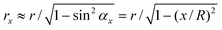 . The adhesion force Fad which is due to the capillary force from a capillary bridge during the retracting movement of the cantilever tip is proportional to the perimeter Sx of the contact area, and hence the diameter rx, Fad∝rx. Meanwhile, the value Dad is proportional to the adhesive force Fad. Therefore, the relationship Dad∝rxis satisfied. From the expression of rx, one can find that the contact line increases with the increasing value of x (horizontal position), which indicates that the adhesion force increases when the tip approaches the edge of the nanobubble.
 | ||
| Fig. 31 Schematic of a simplified cylindrical tip and the nanobubble at different positions of the nanobubble. In the figure, r is the radius of a cylindrical tip, R is the radius of nanobubble, Sx is the perimeter of the contact area. The perimeter of the contact area at the edge is larger than that close to the apex of the nanobubble.12 | ||
Wang et al.115 investigated the contact angle hysteresis and the validity of the use of surface tension for nanobubbles through tip–nanobubble interaction analysis by using force–distance curves. (Note here that the force–distance curves are different from the force modulation curves used in the TMAFM method.) The static, advancing, and receding contact angles of nanobubbles are taken as θs, θadv, and θrec, respectively. A schematic is shown in Fig. 32 to demonstrate the tip–nanobubble interaction in extending and retracting movements. In Fig. 32, γLV is liquid–vapor surface tension, h(x) is the distance between the three phase contact line and bottom of the tip, and α is half of the tip cone angle. First, let us assume the macroscopic concept of contact angle hysteresis (θrec < θs < θadv) is still valid in the length scale of the nanobubbles studied here. Therefore, the component force of surface tension force along the axis of the cantilever tip should be different because of the distinction of θrec and θadv. Taking the perimeter of the three phase contact line as s(x), which is a linear function of h(x) and can be approximately given as
| s(x) = c h(x) | (20) |
| Fγ,e(x) = γLVs(x)cos(α + θrec) | (21) |
| Fγ,r(x) = γLVs(x)cos(α + θadv). | (22) |
 | (23) |
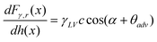 | (24) |
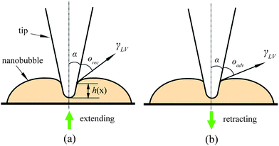 | ||
| Fig. 32 Schematic of tip–nanobubble interaction for (a) extending and (b) retracting movements. The angles α, θrec, and θadv represent half of the tip cone angle, receding contact angle, and advancing contact angle, respectively, and h(x) is the separation distance between three phase contact line and bottom of the tip.115 | ||
With the macroscopic concept of contact angle hysteresis and surface tension, the relationship of eqn (23) and (24) was derived. The next step is to verify the relationship for nanobubble studies. To get a larger interaction distance between the cantilever tip and nanobubbles and to make sure that the type of interaction shown in Fig. 32 occurs in the experiment, it is necessary to generate a larger nanobubble. In this experiment, the larger nanobubble with a height of about 90 nm was obtained with a higher load, as mentioned in the previous research reported by Bhushan et al.12 Then, the force–distance curves were obtained on areas with and without the nanobubble.
The force–distance curves on areas with and without the nanobubble are shown in the left and right images of Fig. 33a, respectively. Most times, the cantilever deflection signal is not flat before getting into hard contact with sample surfaces because optical interference causes it to fluctuate.84 The cantilever deflection component generated by the tip–nanobubble interaction was obtained by subtracting a reference signal from the total cantilever deflection signal on the nanobubble. The average of three force–distance curves shown in the left image of Fig. 33a from different positions without the nanobubble is taken as the reference signal. The three force–distance curves superimpose on each other for extending and retracting movements, especially for the portion before getting contact with the sample surface. However, one can find apparent fluctuations of the cantilever deflection signal on the nanobubble and the distinction between extending and retracting movements, as shown in the right image. Point A in the right image represents a snap-in point, at which the cantilever tip contacts with the nanobubble and the tip begins to penetrate the nanobubble, like the response of the cantilever at the snap-in point in force modulation curves. Point B corresponds to the beginning of the hard contact with the PS film. Point C represents the point at which the cantilever tip overcomes the adhesion force and loses contact with the nanobubble.
 | ||
| Fig. 33 (a) Three force distance curves for both extending and retracting movement obtained on the PS film without nanobubbles (left). The average of the three force–distance curves is taken as the reference cantilever deflection signal for determination of tip–nanobubble component signal. Force–distance curves for both extending and retracting movement on the top of a nanobubble (right). Points A, B, and C represent the points at which the tip contacts with the nanobubble, gets hard contact with the PS film, and loses contact with the nanobubble, respectively. (b) Cantilever deflection signal components solely produced by tip–nanobubble interaction for both extending and retracting movement obtained by subtracting the reference cantilever deflection signal obtained in the left image of (a) from the total cantilever deflection signal in the right image of (a). The distinction between two slopes in the range of piezo vertical position 60 and 120 nm verifies the existence of contact angle hysteresis, as predicted in eqn (23) and (24).115 | ||
Compared with hard contact, the variation of cantilever deflection signal is relatively small, and the cantilever deflection signal is fluctuating. Therefore, it is not accurate if the tip–nanobubble interaction analysis is just based on the curve on the nanobubble itself. Here the reference signal obtained by averaging the three cantilever deflection signals shown in the left image is subtracted from the total cantilever deflection signal obtained on the nanobubble. The cantilever deflection signal component solely produced by the tip–nanobubble interaction is then obtained, as shown in Fig. 33b. During extending and retracting movements, the separation distance h(x) in eqn (23) and (24) is the same distance of the piezo vertical position between the point B and a given tip location in the range of A to B and B to C in the right image of Fig. 33a. From Fig. 33b, it is clear that the signal in the range of 60 to 120 nm piezo vertical position separately follows two slopes of about −0.0178 and −0.0056 for extending and retracting movements, respectively. The existence of two slopes verifies the relationship of eqn (23) and (24). Therefore, one can expect that the concepts of contact angle hysteresis and surface tension should still be used for nanobubbles.
4.5 Nanobubble immobility study
From the point of view of reducing drag force in micro/nanofluidics, it is desirable that nanobubbles stay on the hydrophobic surfaces with limited or no movement, called nanobubble immobility.115 Therefore, improving nanobubble immobility is desirable. Moreover, nanobubble immobility study can also provide further information about the physical interaction between nanobubbles and the substrate supporting them.Wang et al.115 investigated the relationship between nanobubble immobility and surface structures on two kinds of micro/nanostructured surfaces. The first kind of surface was a continuously coated PS film. As mentioned earlier, nanoindents are expected to be generated on the continuously coated PS film after immersion in water for a period of time. Nanobubble immobility was thereafter studied with respect to nanoindents. The second kind of surface was a partially coated PS film which was fabricated by a spin coating method with a low PS concentration. On the partially coated PS film, the hydrophobic structures will coexist with the hydrophilic substrate in the form of island-like structures, and nanobubbles will appear on hydrophobic structures. It was investigated whether island-like structures on partially coated PS film will improve nanobubble immobility. A model was then developed to explain the experimental observation based on contact angle hysteresis and surface tension.
TMAFM images of continuously and partially coated PS films in air are shown in Fig. 34. Unlike the continuously coated PS film, where a smooth PS film is obtained and no surface structures are found, some island-like structures are generated on the partially coated PS film. Additionally, the light dots outside the island-like structures on the partially coated PS film should be PS debris generated during spin coating the surface.
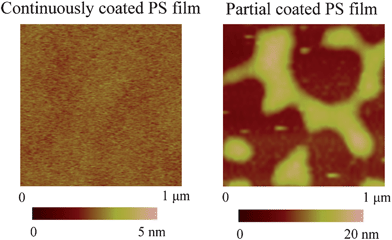 | ||
| Fig. 34 AFM images of continuously coated PS film (left) and partially coated PS film (right) in air. A smooth surface is obtained on the continuously coated PS film, while the island-like structures are obtained on the partially coated PS film.115 | ||
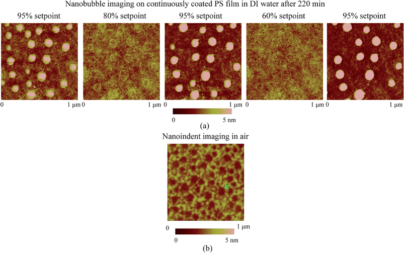 | ||
| Fig. 35 (a) Nanobubble images on the continuously coated PS film as a sequence of applied amplitude setpoints of 95%, 80%, 95%, 60%, and 95% on the same scan area in DI water, and (b) PS film imaged in air after the water was removed from the surface. Some nanobubbles are moved and coalesced by applying an amplitude setpoint of 60%. Arrows indicated in images 3 and 5 in (a) correspond to a nanobubble used in force modulation experiments. Nanoindents were found on the surface after the water was removed and a nanoindent is pointed by an arrow.115 | ||
By comparing the first, the third, and the fifth images in Fig. 35a, one can see that the density of nanobubbles decreases with the increasing size of some nanobubbles, which is the result of nanobubble movement and coalescence.12,115 Although nanobubbles coalesce by sequentially increasing scan load, the response of the nanobubbles to high loads reported here represents improved immobility compared with the nanobubble coalescence observed in the nanobubble imaging section of this paper as well as others95 on a similar PS film. In the experiment performed by Bhushan et al.12 on a similar PS surface, nanobubbles coalesced by increasing the scan load from 95% to 90%. Finally, all nanobubbles were coalesced, generating one single nanobubble in a 2 μm × 2 μm scan area. The difference between the two experiments is the immersion time in water. In the previous research, the experiment was performed within 30 min after immersion in water. However, in this research, the experiments were performed about 220 min after the surface was immersed in water. According to the phenomenon of nanobubble induced nanoindents,116 when a PS film is immersed in water, nanoindents will be induced by high internal pressure combined with surface tension force along the three phase contact line. The generation of nanoindents is dependant on the immersion time in water and nanobubble size. With time, the rim structures gradually increased around the nanobubbles. For the continuously coated PS film studied in this paper, nanoindent generation should also be expected. To verify whether there were nanoindents on the PS film, water was removed from the surface, and then the surface was imaged in air with TMAFM, as shown in Fig. 35b. Nanoindents were found over the surface and an example of a nanoindent is pointed out by an arrow. Compared with PS films without nanoindents, the nanoindents on the PS film are expected to affect nanobubble immobility.
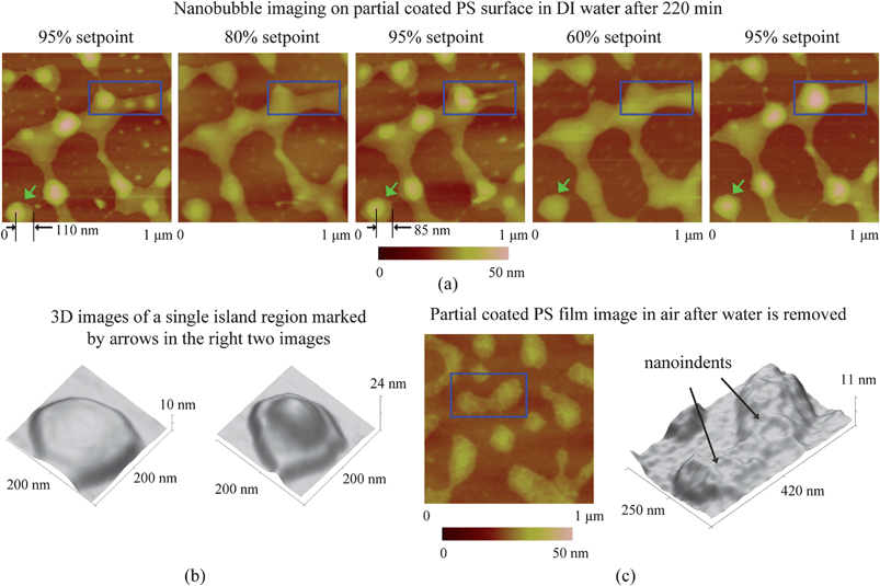 | ||
| Fig. 36 (a) Nanobubble images on the partially coated PS film as a sequence of applied amplitude setpoints of 95%, 80%, 95%, 60%, and 95% on the same scan area in DI water. Three nanobubbles coalesce and generate a big nanobubble in the boxed area, while the other nanobubbles stay on PS islands. The nanobubble pointed to by arrows in the first and third images shows evidence of nanobubble movement based on the measurement of the distance between the center of the nanobubble and edge of the PS island. (b) 3D images for the PS island pointed by the arrows in the fourth and fifth AFM images of (a). In the left image, the nanobubble cannot be imaged because of the penetration of AFM tip into the nanobubble. The image represents the topography of PS island. In the right image, nanobubble is imaged and sits on top of the PS island. (c) AFM image of the partially coated PS film in air after water was removed (left) and corresponding 3D image for the boxed area (right). Nanoindents are found on PS islands as pointed by arrows in the 3D image.115 | ||
A half image of one nanobubble is found in the selected area of the third image. The incomplete nanobubble image is due to nanobubble movement.115 The scan direction of the third image is downward. When the nanobubble was imaged, it was not moved. Therefore, one can still get the nanobubble image. With the perturbation of the AFM tip, it was finally moved and merged into a bigger nanobubble to the right of it. As a result, a half image of the nanobubble with increasing size of the bigger nanobubble in the right was obtained. Therefore, the incomplete nanobubble images can be taken as evidence of nanobubble movement and/or coalescence in TMAFM imaging of nanobubbles. After applying a 60% amplitude setpoint to the area, as shown in the fourth image, the final stage of nanobubbles is shown in the fifth image with 95% amplitude setpoint. A single large nanobubble is finally obtained in the selected area.
One nanobubble sitting on a single PS island is marked by an arrow in the first, third, and fifth images of Fig. 36a. Compared with the nanobubble in the first image, the nanobubble in the third image is moved about 25 nm to the right based on measurement of the distance between the center of the nanobubble and the right edge of the PS single island before (110 nm) and after (85 nm) movement. However, during the process, it does not move out of the PS island and disappear. Nanobubbles on other PS islands do not disappear either. The left and right three dimensional (3D) images in Fig. 36b correspond to the area marked by arrows in the fourth and fifth images of Fig. 36a and show the PS island structure with and without the nanobubble.
As on the continuously coated PS film, nanoindents are expected to be generated on the island-like structures due to nanobubbles. To verify the generation of nanoindents, the surface was imaged in air after water was removed, as shown in Fig. 36c. The right image of Fig. 36c shows a 3D structure of the area selected by a box in the left AFM image. The structures pointed out by arrows are nanoindents generated by nanobubbles, similar to those on the continuously coated PS film reported by Wang et al.116 Therefore, one can expect that the nanoindents on PS islands should also contribute to improved immobility on the partially coated PS film, like on the continuously coated PS film. More importantly, through the above experimental result, one can see that although nanobubble movement and coalescence can occur within island-like structures, none of the nanobubbles moved out of the island structures during experiments. In another words, the island-like structures themselves limit the movement of nanobubbles, which shows improved nanobubble immobility.
Three cases are shown in Fig. 37a, b, and c, which correspond to nanobubbles on a continuously coated PS film without nanoindents, a continuously coated PS film with nanoindents, and a partially coated PS film with island-like structures. In each case, solid and dashed profiles represent nanobubbles statically sitting on the surface and under perturbation of an AFM tip, respectively. Ff and Fb represent components of surface tension forces exerted on the front and back sides of the nanobubble, respectively. The initial force Finit needed to move the nanobubble in each case can be given as Finit = Fb- Ff. Therefore, the mechanism of improved nanobubble immobility can be revealed by comparing Finit in each case.
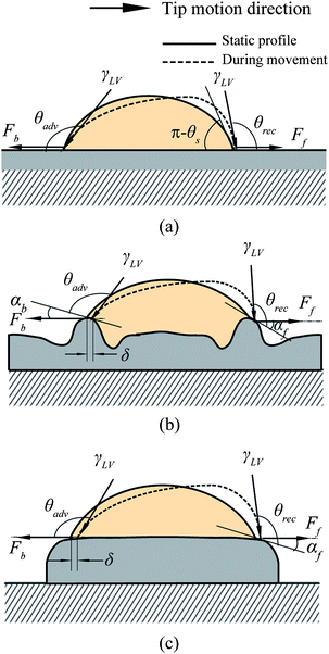 | ||
| Fig. 37 Schematic of movement of a nanobubble on continuously coated PS film without nanoindents (a) and with nanoindents (b) and on partially coated PS film with island-like structures (c). In cases (b) and (c), a finite displacement of δ will lead to the change of the angle of surface tangent relevant to the horizontal plane and hence change the component forces of surface tension along horizontal directions for both front and back side of the nanobubble.115 | ||
Furmidge40 derived an equation describing the relationship between contact angle hysteresis and the sliding angle of a water droplet on a slope, which is widely used to study the movement and manipulation of water droplets.88 The sliding angle is the angle of tilted surface necessary to produce sliding of the water droplet. Based on his analysis, a model to explain nanobubble movement was derived.115 Although water droplets and nanobubbles are different things, it is valid to apply the Furmidge analysis of moving water droplets to nanobubble movement studies, because essentially moving a water droplet and moving a nanobubble deals with the same thing, the three phase contact line. Only if contact angle hysteresis still exists for nanobubbles, which is verified through force–distance curve analysis, could the Furmidge analysis of a moving water droplet be applied to the moving nanobubbles study. According to the tip–nanobubble interaction analysis using force–distance curves, static, advancing, and receding contact angles for nanobubbles follow the same relationship as on the macroscopic scale: θrec < θs < θadv.
Fig. 38 shows the movement of a nanobubble on a flat surface. The dashed and solid profiles represent the nanobubble before and after movement, respectively. Note here the contact angle at the front side of nanobubble movement is the receding contact angle, while the contact angle at the back side is the advancing contact angle. This is opposite from the water droplet case. Because the contact line tension force is along the three phase contact line and is symmetrical and self-equilibrating for the entire contact line, only the external force and surface tension force need to be considered when nanobubble movement is under discussion. Before the nanobubble can be moved, the applied initial horizontal force (Finit marked by a horizontal arrow in Fig. 38) must be big enough to overcome the unbalanced surface tension force produced by the hysteresis of the contact angle (θrec < θadv). When the nanobubble slides the distance dl on the surface without acceleration, the work W done by Finit can be given as
| W = Finitdl | (25) |
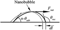 | ||
| Fig. 38 Schematic of a nanobubble sliding on a surface. The dash and solid profile separately represents the droplet before and after the displacement dl. Finit represents the initial force needed to move the nanobubble.115 | ||
Similar to the analysis for moving water droplets,40 the work done by the nanobubble in moving the distance dl can be given as
| W = γLVwdlcos(π − θadv) − γLVwdlcos(π − θrec) | (26) |
| Finit = Fb − Ff = γLVw[cos(π − θadv) − cos(π − θrec)] | (27) |
For case (b) in Fig. 37, it is assumed that a finite virtual displacement δ is made to the nanobubble under the perturbation of a cantilever tip. The change of surface topography resulting from the displacement δ will lead to inclined angles αb and αf of tangential planes for the back and front sides of the nanobubble, respectively, which therefore leads to the angle change of the surface tension force relative to the horizontal direction. Note here that the inclined angles αb and αf are virtual angles assuming the small displacement δ is made to the nanobubble. From a physical point of view, one can expect both the angles π − (θadv + αb) and π − (θrec – αf) should be acute angles. This is based on the following facts. The angle π − (θadv + αb) represents the inclined angle of the surface tension force at the back side of the nanobubble relative to the negative direction of the tip motion (the positive motion direction of the nanobubble is shown by an arrow at the top of Fig. 37). Based on the fact that the curve of the nanobubble is outward, the value of the angle π − (θadv + αb) has to be larger than zero. Additionally, because θadv should be larger than 90° and the angle αb is positive, the angle π − (θadv + αb) is smaller than 90°. Therefore, π − (θadv + αb) is an acute angle. Similarly, π − (θrec – αf) represents the inclined angle of surface tension force at the front side of the nanobubble relative to the positive direction of the tip motion. It is clear that π − (θrec – αf) is larger than zero based on the fact that the curve of the nanobubble is outward. The existence of αf in the angle π − (θrec – αf) makes it larger than π − θrec, except that the angle αf is large enough to make the term π − (θrec – αf) larger than 90°. If so, it will further increase the force needed to move the nanobubble.
The initial force Finit needed to move the nanobubble in case (b) can then be given as
| Finit = Fb − Ff = γLVw[cos(π − (θadv + αb)) − cos(π−(θrec − αf))] | (28) |
For case (c) in Fig. 37, which corresponds to the partially coated PS film, the nanobubble locates on the top of a PS island. When the displacement δ is made, it is assumed that the inclined angle remains unchanged for the back side of the nanobubble, while there is an inclined angle αf for the tangential plane at the front side of the nanobubble due to the displacement δ. Similarly, the initial force Finit needed is given as
| Finit = Fb − Ff = γLVw[cos(π−θadv) − cos(π−(θrec−αf)] | (29) |
From the above analysis, one can see that the presence of nanoindents and island-like structures improves nanobubble immobility through increasing the initial force needed to move nanobubbles compared with smooth hydrophobic surfaces without surface structures.
4.6 Summary
Fig. 39 summarizes the nanobubble study on hydrophobic surfaces. Nanobubbles are sensitive to scan speed and scan load during imaging with TMAFM. Step by step nanobubble coalescence can be achieved by changing either the scan speed or scan load. During coalescence, smaller nanobubbles were easier to move than bigger nanobubbles due to their lower interaction with sample surfaces than that of bigger nanobubbles. The moved nanobubbles then merged into bigger ones and generated new nanobubbles.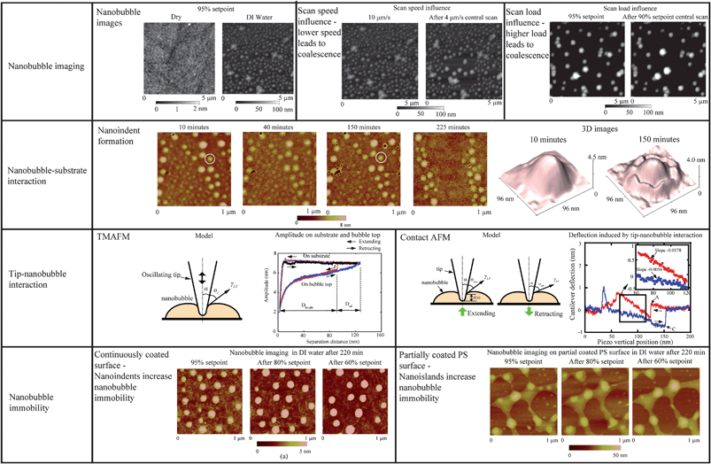 | ||
| Fig. 39 Summary of nanobubble study through aspects of nanobubble imaging, nanobubble–substrate interaction, tip–nanobubble interaction, and nanobubble immobility. | ||
After an immersion time of over 220 min of a thin PS film in DI water, nanobubble induced nanoindents are observed. With time, nanobubbles first shrank and rims appeared around them. Small nanobubbles with diameters less than 50 nm gradually disappeared, leaving nanoindents at their sites. However, bigger nanobubbles with diameters larger than 70 nm were more stable and still remained after 200 min with rims growing around them. The combination of high inner pressure and the perpendicular component of surface tension force along the three phase contact line are believed to be responsible for the appearance of rims and the formation of nanoindents. The size of the nanobubbles is greatly correlated with the speed of nanobubble disappearance and nanoindent formation. Small nanobubbles disappeared at about 150 min. In contrast, big nanobubbles continue to stay on the rims during the experiment. This is believed to be due to the higher inner pressure of small nanobubbles than that of big nanobubbles. Small nanobubbles are also more sensitive to topography change than bigger ones.
Both force modulation and force distance curves can be used to study nanobubble mechanical properties and solid–liquid interaction on the micro/nanoscale. Using force modulation mode, nanobubble height and tip–nanobubble adhesion information can be obtained. Experiments reveal that adhesion force inversely increases with the nanobubble height along nanobubble section profiles with tip–nanobubble interaction. The experimental results obtained using force–distance curves on a nanobubble top reveal that contact angle hysteresis and surface tension force are still valid at the length scale of nanobubbles.
Regarding nanobubble immobility study, experimental results show both nanoindents on continuously coated PS film and nanoisland structures on partially coated PS film improve nanobubble immobility. A model is developed to reveal the mechanism of the improved nanobubble immobility based on contact angle hysteresis and surface tension. Analysis shows that nanoindents and nanoislands on the films will increase the initial force needed to move nanobubbles. Hence, nanobubble immobility is improved on both surfaces as compared with smooth hydrophobic surfaces.
5. Liquid micro droplet sliding with presence of electric field
As stated in the Introduction, the measurement of sliding forces can provide evidence for the quantitative evaluation of the capability of liquid droplet sliding on specified surfaces, which is of significance for liquid manipulation related micro/nanofluidics applications. In this section, a method of quantitative measurement of liquid droplet sliding force with the presence of an electric field using atomic force microscopy will be discussed based on Wang and Bhushan.1135.1 Experimental
The droplet sliding experiments were performed by Wang and Bhushan113 on a polystyrene (PS) surface spin coated on a p-type boron doped silicon wafer (1–20 Ω cm, Silicon Quest International) with a 300 nm thick silicon oxide coating grown thermally on the wafer. The silicon oxide wafer was first cleaned in a sonication bath of acetone and then water before spin-coating. PS film with a thickness of about 60 nm obtained using spin coating method is taken as the hydrophobic surface. After that, the PS surface was glued to a metal AFM sample plate with conductive silver paint to make sure the doped silicon substrate and the sample plate was electrically connected.The droplet sliding experiment was performed with a commercial AFM. An n-type silicon (0.5–2 Ω cm) cantilever with a nominal spring constant of 3 N/m and tip radius less than 10 nm was used to slide liquid droplets. The liquid is a mixture of water, glycerin, and sodium chloride (NaCl). The glycerin was added to keep droplets from evaporating in the ambient environment, whereas the NaCl was added to make the liquid conductive in order to perform the electrowetting experiment. The static contact angle was measured with a sessile drop method, as shown in Fig. 40 (left). To measure dynamic contact angle, the glycerin drop was put on an inclined PS surface. The incline angle was gradually increased until the liquid drop started to slide and then the image was taken, as shown in Fig. 40 (right). The advancing and receding contact angles measured from the profile of sliding profile at lower contact line and upper contact line were 98.9 ± 2.3° and 60.3 ± 1.7°, respectively.
 | ||
| Fig. 40 Images of a static glycerin droplet (left) on a horizontal surface and a sliding glycerin droplet (right) on an inclined surface with PS spin coated on SiO2 substrate. The static and dynamic contact angles can then be measured from the profiles of the static and dynamic droplets, respectively. The obtained static, advancing, and receding contact angles are 82.2°, 98.9°, and 60.3°, respectively.113 | ||
Before performing the droplet sliding experiment, the AFM cantilever was first used to laterally scan on a silicon (100) substrate to calibrate lateral friction force using a method called the pivot method.25,113 The conversion factor which converts lateral deflection signal to friction force was obtained as 1.40 × 10⁴ nN/V. During the experiment, there is a separation distance of 3 μm between the bottom of the tip and the sample surface. Therefore the conversion factor C needs to be adjusted. The corrected one is about 1.05 × 10⁴ nN/V. To deposit small droplets and then conduct the droplet sliding experiment, a small amount of the liquid mixed with large amount of air was quickly sprayed on the PS sample.10 Droplets with diameters of less than 100 μm were obtained on the surface. Before sliding, the relative positions between the cantilever tip and target liquid droplets were adjusted by adjusting the positions of the sample stage with the integrated function of the Dimension AFM. Then, droplets with different sizes were first lined up through cantilever tip manipulation, then slid by the cantilever tip. The sliding speed is 100 μm s−1. Here, one should make sure all liquid in a droplet slides with the cantilever tip, otherwise the friction force will be underestimated due to the decreased size of the droplets. By optical microscopy observation, it is found to be satisfied on the PS surface, and the PS surface remains dry after droplets slide over.
To investigate the impact of applied potentials on droplet sliding, applied potentials in the range of 0–80 V were applied between the cantilever tip and the sample substrate using a DC power supply (E3612A, HP), and the sample substrate was connected to ground of the power supply.
5.2. Impact of electrowetting on micro droplets
Fig. 41a left and right show a liquid droplet before and after the potentials are applied between the tip and the substrate.113θY and θV, w1 and w2 are static contact angles and width of the droplet before and after the potential V is applied, and d is the separation distance between the bottom of the cantilever tip and the sample surface of the PS film.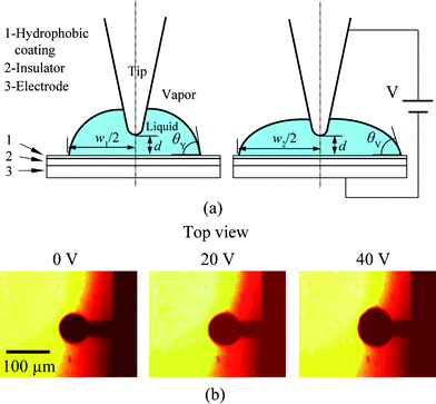 | ||
| Fig. 41 (a) Schematic of a liquid droplet without (left) and with (right) an applied potential V. Before applying V, the contact angle is θY with diameter of w1. When V is applied, the contact angle decreases to θV, and diameter of the droplet increases to w2. During experiment, the distance d between the bottom of the tip and the sample surface is kept as 3 μm. (b) Top view of a droplet attached by the AFM cantilever with different applied potentials. The diameter increases with increasing potentials.113 | ||
The presence of V reduces interface tension and hence reduces the static contact angle. When V is applied between the droplet and doped silicon substrate, the contact angle θV of the droplet can be expressed by the so-called Lippmann equation,76
 | (30) |
In addition to the decrease of contact angle demonstrated in Fig. 41a, the width of the droplet is expected to increase due to the decrease of the contact angle. To verify the change of the width, the cantilever is first attached to a droplet with a diameter of about 60 μm, as shown in Fig. 41b. Then, the applied voltages are increased to 20 V and 40 V. It is clear that the size of droplet increases with applied potentials. From eqn (30), one can see that in addition to electric potential V, the thickness td also influences the variation of contact angle. When the thickness decreases, the contact angle will further decrease. Correspondingly, the width of droplets will increase.
5.3 Sliding of droplets with different size
When liquid droplets are slid, the driving force is provided by the cantilever tip.113Fig. 42 demonstrates a droplet sliding without (left) and with (right) an applied potential. During sliding, the front side and back side contact angle of the droplet are expected to be the advancing and receding contact angles of the droplet.88 Therefore, the angles θY,a, θV,a, and θY,r, θV,r are advancing and receding contact angles for the droplet without and with the applied potential, respectively.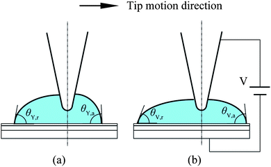 | ||
| Fig. 42 Schematic of a liquid droplet sliding by the motion of the AFM tip without (left) and with (right) the potential V. θY, a and θY, r are advancing and receding contact angles without V, while θV, a and θV, r are advancing and receding contact angles with V.113 | ||
The immersion of an AFM tip into the droplet may change the profile of the droplet, which will further change the width of the droplet. Therefore, it is necessary to check the portion of the AFM tip immersed into liquid droplet. Wang and Bhushan113 reported that according to the geometry of the cantilever tip used and experimental setup, during working, the volume of cantilever tip immersed into the liquid droplet takes less than 5% of the liquid droplet volume for each droplet. Therefore, the width of the droplet before the immersion of the cantilever tip can be approximately taken as the value during liquid droplet sliding. Similar to the treatment of nanobubble movement as mentioned in the section of nanobubble immobility, the initial forces FY,init and FV,init needed to drive the droplet without and with the applied potential can be separately given as,113
| FY,init = γLVw1(cosθY,r − cosθY,a) | (31) |
| FV,init = γLVw2(cosθV,r − cosθV,a) | (32) |
Four droplets with diameters less than 30 μm were slid by Wang and Bhushan,113 as shown in the inset image of Fig. 43. The droplets were first lined up in a sequence of increasing size. Then they were separately slid without applied potentials. After that, 20 V potential was applied between the tip and the substrate. The lateral friction force for droplets without and with the 20 V potential are plotted in Fig. 43. Without the potential, friction force linearly increases with droplet diameters, as indicated by eqn (31). After the 20 V potential is applied, the friction force also increases with increasing droplet diameter. More importantly, the applied potential greatly increases the friction force for each droplet. To further investigate the impact of applied potentials on lateral friction force, different potentials were applied to a droplet with a diameter of about 16.5 μm. The friction force as a function of applied potentials is plotted in Fig. 44. Friction forces are also found to increase with applied potentials. The phenomenon of increased friction force with applied potentials is consistent with the increasing diameter of droplets induced by the applied potentials as shown in Fig. 41b. As mentioned earlier, since the thickness of insulator will change the contact angle and hence the width of droplets, in addition to applied electric field, one can also increase the sliding force through decreasing the thickness of the coating. From the point of view of reducing sliding force, because the composite interface between droplets and superhydrophobic surfaces can greatly decrease contact angle hysteresis and hence reduce sliding force,9 the superhydrophobic surfaces are desirable. However, whether the composite interface exists or not depends on droplet size and distribution of microstructures on the superhydrophobic surfaces,70,63 the selection of liquid droplet should be consistent with surface structures to generate composite interfaces.
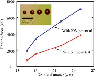 | ||
| Fig. 43 Friction force as a function of droplet diameters with and without 20 V potential when droplets are slid by the cantilever tip. Friction force increases with droplet size as well as with the applied potential. The inset shows optical image of droplets with different sizes.113 | ||
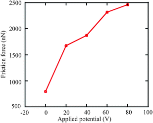 | ||
| Fig. 44 Friction force as a function of applied potential. The friction force increases with applied potentials.113 | ||
6. Outlook
We have reviewed the recent development of boundary slip and nanobubble study using AFM. Both contact mode AFM and TMAFM can be used to study boundary slip at solid–liquid interfaces through slip length measurement. No-slip boundary condition on hydrophilic surfaces was found in liquid drainage experiments using the contact mode AFM method. For hydrophobic and superhydrophobic surfaces, experimental results show velocity independence of boundary slip by performing drainage experiments with different approach velocities. Slip lengths of 44 and 257 nm were obtained with the contact mode AFM method for hydrophobic and superhydrophobic surfaces, respectively, which are close to the values of 43 and 236 nm obtained with TMAFM. The experimental results on surfaces with different hydrophobicities demonstrate increasing boundary slip with hydrophobicity of sample surface.As a possible reason for boundary slip, nanobubbles can be correlated with boundary slip. By imaging nanobubbles on the hydrophobic surfaces, the measured slip length on the surface can be explained by approximately treating the intermittent nanobubbles as a continuous gas layer with an efficient thickness, which provides an approach to reveal the influence of nanobubbles on boundary slip. Nanobubbles are found to be sensitive to scan parameters during imaging. Step by step nanobubble coalescence can be achieved by changing either the scan speed or scan load. Both force modulation and force distance curves can be used to study nanobubble mechanical properties and solid–liquid interaction on micro/nanoscale. The experimental results obtained using force distance curves on a nanobubble top reveal that contact angle hysteresis and surface tension force are still valid at the length scale of nanobubbles. Nanobubbles are found to influence the substrates supporting them and nanobubble induced nanoindents can be observed. The combination of high inner pressure and the perpendicular component of surface tension force along the three phase contact line is believed to be responsible for the formation of the nanoindents. The generated nanoindents are expected to influence nanobubble immobility. Experimental results show both nanoindents on continuously coated PS film and nanoisland structures on partially coated PS film improve nanobubble immobility as compared with smooth hydrophobic surfaces.
Although nanobubbles are thought to be a reason for boundary slip on hydrophobic surfaces, more effort needs to be made to further verify the role of nanobubble on boundary slip through experiments and simulations. In practice, it is difficult to study both nanobubbles and boundary slip for rough sample surfaces. One way to study the relationship between nanobubbles and boundary slip is by using liquid drainage experiments with an AFM. However, because nanobubbles are fragile, they may be destroyed during the liquid drainage experiments. The production of nanobubbles is found to be irreproducible, and they are sensitive to the surface properties, such as roughness and hydrophobicity, which makes the study complicated. Therefore, the controllable formation of nanobubbles is desirable for both boundary slip and nanobubble studies.
Acknowledgements
Yuliang Wang acknowledges financial support from Chinese Scholarship Council. Authors thank Dr Abdelhamid Maali for extensive help and many useful discussions.References
- J. L. Barrat and L. Bocquet, Large slip effect at a nonwetting fluid-solid interface, Phys. Rev. Lett., 1999, 82, 4671–4674 CrossRef CAS
.
-
G. K. Batchelor, An Introduction to Fluid Dynamics, Cambridge University Press, Cambridge, England, 1970 Search PubMed
- J. Baudry, E. Charlaix, A. Tonck and D. Mazuyer, Experimental evidence for a large slip effect at a nonwetting fluid-solid interface, Langmuir, 2001, 17, 5232–5236 CrossRef CAS
- D. Bernoulli, Hydrodynamica, 1738 Search PubMed
-
B. Bhushan, Principles and Applications of Tribology(Wiley, New York, 1999) Search PubMed
-
B. Bhushan, Introduction to Tribology, Wiley, New York, 2002 Search PubMed
-
B. Bhushan, Springer Handbook of Nanotechnology, second edn, Springer, Heidelberg, Germany, 2007 Search PubMed
-
B. Bhushan, Nanotribology And Nanomechanics: An Introduction, second edn, Springer, Heidelberg, Germany, 2008 Search PubMed
- B. Bhushan and Y. C. Jung, Wetting, adhesion and friction of superhydrophobic and hydrophilic leaves and fabricated micro/nanopatterned surfaces, J. Phys.: Condens. Matter, 2008, 20, 225010 CrossRef
- B. Bhushan and X. Ling, Integrating electrowetting into micromanipulation of liquid droplets, J. Phys.: Condens. Matter, 2008, 20, 485009 CrossRef
- B. Bhushan and X. Ling, Manipulating microobject by using liquid droplet as a transporting vehicle, J. Colloid Interface Sci., 2009, 329, 196–201 CrossRef CAS
- B. Bhushan, Y. Wang and A. Maali, Coalescence and Movement of Nanobubbles studied with Tapping Mode AFM and Tip-bubble Interaction Analysis, J. Phys.: Condens. Matter, 2008, 20, 485004 CrossRef
- B. Bhushan, K. Koch and Y. C. Jung, Nanostructures for superhydrophobicity and low adhesion, Soft Matter, 2008, 4, 1799–1804 RSC
- B. Bhushan, Y. C. Jung and K. Koch, Micro-, nano- and hierarchical structures for superhydrophobicity, self-cleaning and low adhesion, Philos. Trans. R. Soc. London, Ser. A, 2009, 367, 1631–1672 CrossRef CAS
- B. Bhushan, Y. Wang and A. Maali, Boundary Slip Study on Hydrophilic, Hydrophobic, and Superhydrophobic Surfaces with Dynamic Atomic Force Microscopy, Langmuir, 2009, 25, 8117–8121 CrossRef CAS
- E. Bonaccurso, M. Kappl and H. J. Butt, Hydrodynamic force measurements: Boundary slip of water on hydrophilic surfaces and electrokinetic effects, Phys. Rev. Lett., 2002, 88, 076103 CrossRef
- E. Bonaccurso, H. J. Butt and V. S. J. Craig, Surface roughness and hydrodynamic boundary slip of a newtonian fluid in a completely wetting system, Phys. Rev. Lett., 2003, 90, 144501 CrossRef
- B. M. Borkent, S. M. Dammer, H. Schonherr, G. J. Vancso and D. Lohse, Superstability of surface nanobubbles, Phys. Rev. Lett., 2007, 98, 204502 CrossRef
- E. Bormashenko, On the role of contact line tension and 2D defects in the formation of the water depletion layer on hydrophobic surfaces, Chem. Phys. Lett., 2008, 456, 186–188 CrossRef CAS
- E. Bormashenko, R. Pogreb, G. Whyman and M. Erlich, Cassie-wenzel wetting transition in vibrating drops deposited on rough surfaces: Is the dynamic Cassie–Wenzel wetting transition a 2D or 1D affair?, Langmuir, 2007, 23, 6501–6503 CrossRef CAS
-
R. H. Boundy and R. F. E. Boyer, Styrene, Its Polymers, Copolymers and Derivatives, Reinhold, New York, 1952 Search PubMed
-
J. Brandrup, E. H. Immergut and E. A. Grulke, Polymer Handbook, Wiley, New York, 1999 Search PubMed
- H. R. Brown and T. P. Russell, Entanglements at polymer surfaces and interfaces, Macromolecules, 1996, 29, 798–800 CrossRef CAS
- M. A. Burns, B. N. Johnson, S. N. Brahmasandra, K. Handique, J. R. Webster, M. Krishnan, T. S. Sammarco, P. M. Man, D. Jones, D. Heldsinger, C. H. Mastrangelo and D. T. Burke, An integrated nanoliter DNA analysis device, Science, 1998, 282, 484–487 CrossRef CAS
- R. G. Cain, S. Biggs and N. W. Page, Force calibration in lateral force microscopy, J. Colloid Interface Sci., 2000, 227, 55–65 CrossRef CAS
- A. Carambassis, L. C. Jonker, P. Attard and M. W. Rutland, Forces measured between hydrophobic surfaces due to a submicroscopic bridging bubble, Phys. Rev. Lett., 1998, 80, 5357–5360 CrossRef CAS
- M. K. Chaudhury and G. M. Whitesides, How to Make Water Run Uphill, Science, 1992, 256, 1539–1541 CrossRef CAS
- X. Chen, M. C. Davies, C. J. Roberts, S. J. B. Tendler, P. M. Williams, J. Davies, A. C. Dawkes and J. C. Edwards, Interpretation of tapping mode atomic force microscopy data using amplitude-phase-distance measurements, Ultramicroscopy, 1998, 75, 171–181 CrossRef CAS
- J. H. J. Cho, B. M. Law and F. Rieutord, Dipole-dependent slip of Newtonian liquids at smooth solid hydrophobic surfaces, Phys. Rev. Lett., 2004, 92, 166102 CrossRef
- S. K. Cho, H. J. Moon and C. J. Kim, Creating, transporting, cutting, and merging liquid droplets by electrowetting-based actuation for digital microfluidic circuits, Journal of Microelectromechanical Systems, 2003, 12, 70–80 CrossRef
- C. H. Choi and C. J. Kim, Large slip of aqueous liquid flow over a nanoengineered superhydrophobic surface, Phys. Rev. Lett., 2006, 96, 066001 CrossRef
- H. K. Christenson and P. M. Claesson, Direct measurements of the force between hydrophobic surfaces in water, Adv. Colloid Interface Sci., 2001, 91, 391–436 CrossRef CAS
- N. V. Churaev, V. D. Sobolev and A. N. Somov, Slippage of Liquids over Lyophobic Solid-Surfaces, J. Colloid Interface Sci., 1984, 97, 574–581 CrossRef CAS
- C. Cottin-Bizonne, C. Barentin, E. Charlaix, L. Bocquet and J. L. Barrat, Dynamics of simple liquids at heterogeneous surfaces: Molecular-dynamics simulations and hydrodynamic description, Eur. Phys. J. E, 2004, 15, 427–438 CrossRef CAS
- C. Cottin-Bizonne, B. Cross, A. Steinberger and E. Charlaix, Boundary slip on smooth hydrophobic surfaces: Intrinsic effects and possible artifacts, Phys. Rev. Lett., 2005, 94, 056102 CrossRef CAS
- V. S. J. Craig, C. Neto and D. R. M. Williams, Shear-dependent boundary slip in an aqueous Newtonian liquid, Phys. Rev. Lett., 2001, 87, 054504 CrossRef CAS
- S. Daniel, M. K. Chaudhury and J. C. Chen, Fast drop movements resulting from the phase change on a gradient surface, Science, 2001, 291, 633–636 CrossRef CAS
- P. L. G. Du Buat, Principes d′ Hydraulique, 1786 Search PubMed
- P. D. I. Fletcher, S. J. Haswell, E. Pombo-Villar, B. H. Warrington, P. Watts, S. Y. F. Wong and X. L. Zhang, Micro reactors: principles and applications in organic synthesis, Tetrahedron, 2002, 58, 4735–4757 CrossRef CAS
- C. G. L. Furmidge, Studies at phase interfaces. I. The sliding of liquid drops on solid surfaces and a theory for spray retention, J. Colloid Sci., 1962, 17, 309–324 CrossRef CAS
-
S. Goldstein, Modern Development in Fluid Dynamics, Clarendon, Oxford, 1938 Search PubMed
- S. Goldstein, Fluid Mechanics in First Half of This Century, Annu. Rev. Fluid Mech., 1969, 1, 1–28 CrossRef
- H. Helmholtz and G. Pictowsky, Uber Reibung tropfbarer Flussigkeiten, Sitzungsber. Kais. Akad. Wiss. Wein, Math.-Naturwiss. Kl., Abt. 2, 1868, 40 Search PubMed
- M. Holmberg, A. Kuhle, J. Garnaes, K. A. Morch and A. Boisen, Nanobubble trouble on gold surfaces, Langmuir, 2003, 19, 10510–10513 CrossRef CAS
- C. D. F. Honig and W. A. Ducker, No-slip hydrodynamic boundary condition for hydrophilic particles, Phys. Rev. Lett., 2007, 98, 028305 CrossRef
- X. Hong, X. F. Gao and L. Jiang, Application of superhydrophobic surface with high adhesive force
in no lost transport of superparamagnetic microdroplet, J. Am. Chem. Soc., 2007, 129, 1478–1479 CrossRef CAS
- K. Ichimura, S. K. Oh and M. Nakagawa, Light-driven motion of liquids on a photoresponsive surface, Science, 2000, 288, 1624–1626 CrossRef CAS
- N. Ishida, T. Inoue, M. Miyahara and K. Higashitani, Nano bubbles on a hydrophobic surface in water observed by tapping-mode atomic force microscopy, Langmuir, 2000, 16, 6377–6380 CrossRef CAS
-
J. Israelachvili, Intermolecular & Surface Forces, 3rd edn,Academic Press, London, 1992 Search PubMed
- J. Israelachvili and R. Pashley, The Hydrophobic Interaction Is Long-Range, Decaying Exponentially with Distance, Nature, 1982, 300, 341–342 CAS
- C. Jai, T. Cohen-Bouhacina and A. Maali, Analytical description of the motion of an acoustic-driven atomic force microscope cantilever in liquid, Appl. Phys. Lett., 2007, 90, 113512 CrossRef
- T. R. Jensen, M. O. Jensen, N. Reitzel, K. Balashev, G. H. Peters, K. Kjaer and T. Bjornholm, Water in contact with extended hydrophobic surfaces: Direct evidence of weak dewetting, Phys. Rev. Lett., 2003, 90, 086101 CrossRef
- P. Joseph and P. Tabeling, Direct measurement of the apparent slip length, Phys. Rev. E: Stat., Nonlinear, Soft Matter Phys., 2005, 71, 035303 CrossRef
- P. Joseph, C. Cottin-Bizonne, J. M. Benoit, C. Ybert, C. Journet, P. Tabeling and L. Bocquet, Slippage of water past superhydrophobic carbon nanotube forests in microchannels, Phys. Rev. Lett., 2006, 97, 156104 CrossRef CAS
- Y. C. Jung and B. Bhushan, “Biomimetic Structures for Fluid Drag Reduction in Laminar and Turbulent Flows” J. Phys.: Condens. Matter, 2009, in press Search PubMed.
- K. Koch, B. Bhushan, Y. C. Jung and W. Barthlott, Fabrication of artificial Lotus leaves and significance of hierarchical structure for superhydrophobicity and low adhesion, Soft Matter, 2009, 5, 1386–1393 RSC
- T. Koishi, S. Yoo, K. Yasuoka, X. C. Zeng, T. Narumi, R. Susukita, A. Kawai, H. Furusawa, A. Suenaga, N. Okimoto, N. Futatsugi and T. Ebisuzaki, Nanoscale hydrophobic interaction and nanobubble nucleation, Phys. Rev. Lett., 2004, 93, 185701 CrossRef CAS
- P. Lambert and A. Delchambre, A study of capillary forces as a gripping principle, Assem. Autom., 2005, 25, 275–283 CrossRef
- D. Lasne, A. Maali, Y. Amarouchene, L. Cognet, B. Lounis and H. Kellay, Velocity profiles of water flowing past solid glass surfaces using fluorescent nanoparticles and molecules as velocity probes, Phys. Rev. Lett., 2008, 100, 214502 CrossRef CAS
- E. Lauga and H. A. Stone, Effective slip in pressure-driven Stokes flow, J. Fluid Mech., 2003, 489, 55–77 Search PubMed
-
E. Lauga, M. P. Brenner and H. A. Stone, Handbook of Experimental Fluid Dynamics, American Chemical Society, New York, 2005 Search PubMed
- S. W. Lee and P. E. Laibinis, Directed movement of liquids on patterned surfaces using noncovalent molecular adsorption, J. Am. Chem. Soc., 2000, 122, 5395–5396 CrossRef CAS
- W. Li and A. Amirfazli, A thermodynamic approach for determining the contact angle hysteresis for superhydrophobic surfaces, J. Colloid Interface Sci., 2005, 292, 195–201 CrossRef CAS
-
D. R. Lide, CRC Handbook of Chemistry and Physics, 90th edn, CRC Press Inc., Boca Raton, FL, 2009 Search PubMed
- S. T. Lou, Z. Q. Ouyang, Y. Zhang, X. J. Li, J. Hu, M. Q. Li and F. J. Yang, Nanobubbles on solid surface imaged by atomic force microscopy, J. Vac. Sci. Technol., B, 2000, 18, 2573–2575 CrossRef CAS
- A. Maali, C. Hurth, T. Cohen-Bouhacina, G. Couturier and J. P. Aime, Improved acoustic excitation of atomic force microscope cantilevers in liquids, Appl. Phys. Lett., 2006, 88, 163504 CrossRef
- A. Maali and B. Bhushan, Nanorheology and boundary slip in confined liquids using atomic force microscopy, J. Phys.: Condens. Matter, 2008, 20, 315201 CrossRef
- A. Maali, Y. Wang and B. Bhushan, Evidence of no-slip boundary condition of water flow between hydrophilic surfaces using atomic force microscopy, Langmuir, 2009, 25, 12002–12005 CrossRef CAS
-
J. E. Mark, Polymer data handbook, Oxford University Press, Oxford, 1999 Search PubMed
- A. Marmur, Wetting on hydrophobic rough surfaces: To be heterogeneous or not to be?, Langmuir, 2003, 19, 8343–8348 CrossRef CAS
- G. A. Matei, E. J. Thoreson, J. R. Pratt, D. B. Newell and N. A. Burnham, Precision and accuracy of thermal calibration of atomic force microscopy cantilevers, Rev. Sci. Instrum., 2006, 77, 083703 CrossRef
- J. C. Maxwell, On Stresses in rarefied gases arising from inequalities of temperature, Philos. Trans. R. Soc. London, 1879, 170, 231–256 CrossRef
- C. D. Meinhart, S. T. Wereley and J. G. Santiago, PIV measurements of a microchannel flow, Exp. Fluids, 1999, 27, 414–419 CrossRef
- H. Meyer, T. Kreer, A. Cavallo, J. P. Wittmer and J. Baschnagel, On the dynamics and disentanglement in thin and two-dimensional polymer films, Eur. Phys. J. Spec. Top., 2007, 141, 167–172 Search PubMed
- K. B. Migler, H. Hervet and L. Leger, Slip Transition of a Polymer Melt under Shear-Stress, Phys. Rev. Lett., 1993, 70, 287–290 CrossRef CAS
- F. Mugele and J. C. Baret, Electrowetting: From basics to applications, J. Phys.: Condens. Matter, 2005, 17, R705–R774 CrossRef CAS
- C. L. M. H. Navier, Memoire sur les lois du mouvement des fluides, Memoires de l'Academie Royale des sciences de l'Institut de France VI, 1823, 389–440 Search PubMed
- C. Neto, D. R. Evans, E. Bonaccurso, H. J. Butt and V. S. J. Carig, Boundary slip in Newtonian liquids: a review of experimental studies, Rep. Prog. Phys., 2005, 68, 2859–2897 CrossRef CAS
-
M. Nosonovsky and B. Bhushan, Multiscale Dissipative Mechanisms and Hierarchical Surfaces: Friction, Superhydrophobicity, and Biomimetics, Springer, Heidelberg, Germany, 2008 Search PubMed
- K. J. Obata, T. Motokado, S. Saito and K. Takahashi, A scheme for micro-manipulation based on capillary force, J. Fluid Mech., 2004, 498, 113–121 Search PubMed
- J. Ou, B. Perot and J. P. Rothstein, Laminar drag reduction in microchannels using ultrahydrophobic surfaces, Phys. Fluids, 2004, 16, 4635–4643 Search PubMed
- R. Pit, H. Hervet and L. Leger, Friction and slip of a simple liquid at a solid surface, Tribol. Lett., 1999, 7, 147–152 CrossRef CAS
- R. Pit, H. Hervet and L. Leger, Direct experimental evidence of slip in hexadecane: Solid interfaces, Phys. Rev. Lett., 2000, 85, 980–983 CrossRef CAS
- M. A. Poggi, J. S. Boyles and L. A. Bottomley, Measuring the compression of a carbon nanospring, Nano Lett., 2004, 4, 1009–1016 CrossRef CAS
- M. G. Pollack, R. B. Fair and A. D. Shenderov, Electrowetting-based actuation of liquid droplets for microfluidic applications, Appl. Phys. Lett., 2000, 77, 1725–1726 CrossRef CAS
- A. Poynor, L. Hong, I. K. Robinson, S. Granick, Z. Zhang and P. A. Fenter, “How water meets a hydrophobic surface”, Phys. Rev. Lett., 2006, 97, 266101 CrossRef
- C. Quilliet and B. Berge, Electrowetting: a recent outbreak, Curr. Opin. Colloid Interface Sci., 2001, 6, 34–39 CrossRef CAS
- P. Roura and J. Fort, Comment on “effects of the surface roughness on sliding angles of water droplets on superhydrophobic surfaces”, Langmuir, 2002, 18, 566–569 CrossRef CAS
- S. Saito, T. Motokado, K. J. Obata and K. Takahashi, Capillary force with a concave probe-tip for micromanipulation, Appl. Phys. Lett., 2005, 87, 234103 CrossRef
- M. Sakamoto, Y. Kanda, M. Miyahara and K. Higashitani, Origin of long-range attractive force between surfaces hydrophobized by surfactant adsorption, Langmuir, 2002, 18, 5713–5719 CrossRef CAS
- M. Sbragaglia and A. Prosperetti, Effective velocity boundary condition at a mixed slip surface, J. Fluid Mech., 2007, 578, 435–451 Search PubMed
- T. Schmatko, H. Hervet and L. Leger, Friction and slip at simple fluid-solid interfaces: The roles of the molecular shape and the solid-liquid interaction, Phys. Rev. Lett., 2005, 94, 244501 CrossRef
- E. Schnell, Slippage of Water over Nonwettable Surfaces, J. Appl. Phys., 1956, 27, 1149–1152 CrossRef
- L. Si, M. V. Massa, K. Dalnoki-Veress, H. R. Brown and R. A. L. Jones, Chain entanglement in thin freestanding polymer films, Phys. Rev. Lett., 2005, 94, 127801 CrossRef
- A. C. Simonsen, P. L. Hansen and B. Klosgen, Nanobubbles give evidence of incomplete wetting at a hydrophobic interface, J. Colloid Interface Sci., 2004, 273, 291–299 CrossRef CAS
- T. G. Stange, R. Mathew, D. F. Evans and W. A. Hendrickson, Scanning Tunneling Microscopy and Atomic Force Microscopy Characterization of Polystyrene Spin-Coated onto Silicon Surfaces, Langmuir, 1992, 8, 920–926 CrossRef CAS
- R. Steitz, T. Gutberlet, T. Hauss, B. Klosgen, R. Krastev, S. Schemmel, A. C. Simonsen and G. H. Findenegg, Nanobubbles and their precursor layer at the interface of water against a hydrophobic substrate, Langmuir, 2003, 19, 2409–2418 CrossRef CAS
- S. G. G. Stokes, On the theories of the internal friction of fluids in motion, and of the equilibrium and motion of elastic solids, Trans. Cambridge Philos. Soc., 1849, 8, 287–319 Search PubMed
- S. G. G. Stokes, On the Effect of the Internal Friction of Fluids on the Motion of Pendulums, Trans. Cambridge Philos. Soc., 1851, 9, 8–106 Search PubMed
- M. Switkes and J. W. Ruberti, Rapid cryofixation/freeze fracture for the study of nanobubbles at solid-liquid interfaces, Appl. Phys. Lett., 2004, 84, 4759–4761 CrossRef CAS
- W. C. Tang and A. P. Lee, Defense applications of MEMS, MRS Bulletin, 2001, 26, 318–319
- T. Thorsen, S. J. Maerkl and S. R. Quake, Microfluidic large-scale integration, Science, 2002, 298, 580–584 CrossRef CAS
- J. Traube and S. H. Whang, Uber reibungskonstante und wandschicht, Z. Physikal Chem. A, 1928, 138, 102–122 Search PubMed
- D. C. Tretheway and C. D. Meinhart, Apparent fluid slip at hydrophobic microchannel walls, Phys. Fluids, 2002, 14, L9–L12 CrossRef CAS
- D. C. Tretheway and C. D. Meinhart, A generating mechanism for apparent fluid slip in hydrophobic microchannels, Phys. Fluids, 2004, 16, 1509–1515 Search PubMed
- J. W. G. Tyrrell and P. Attard, Atomic force microscope images of nanobubbles on a hydrophobic surface and corresponding force-separation data, Langmuir, 2002, 18, 160–167 CrossRef
- M. A. Unger, H. P. Chou, T. Thorsen, A. Scherer and S. R. Quake, Monolithic microfabricated valves and pumps by multilayer soft lithography, Science, 2000, 288, 113–116 CrossRef CAS
- O. D. Velev, B. G. Prevo and K. H. Bhatt, On-chip manipulation of free droplets, Nature, 2003, 426, 515–516 CrossRef CAS
- E. Villari, Introno all'efflusso del mercurio per tubi di vetro di piccolissimo diametro, Accademia delle Scienze dell Instituto di Bologna, 1875, 6 Search PubMed
- A. Vinckier, C. Dumortier, Y. Engelborghs and L. Hellemans, Dynamical and mechanical study of immobilized microtubules with atomic force microscopy, J. Vac. Sci. Technol., B, 1996, 14, 1427–1431 CrossRef CAS
- O. I. Vinogradova, Drainage of a Thin Liquid-Film Confined between Hydrophobic Surfaces, Langmuir, 1995, 11, 2213–2220 CrossRef CAS
- O. I. Vinogradova and G. E. Yakubov, Dynamic effects on force measurements. 2. Lubrication and the atomic force microscope, Langmuir, 2003, 19, 1227–1234 CrossRef CAS
- Y. Wang and B. Bhushan, Liquid micro droplet sliding on hydrophobic surfaces in the presence of electric field, Langmuir, 2009 DOI:10.1021/la903460a
- Y. Wang, B. Bhushan and A. Maali, AFM measurement of boundary slip on hydrophilic, hydrophobic and superhydrophobic surfaces, J. Vac. Sci. Technol., A, 2009, 27, 754–760 CrossRef CAS
- Y. Wang, B. Bhushan and X. Zhao, Improved nanobubble immobility induced by surface structures on hydrophobic surfaces, Langmuir, 2009, 25, 9328–9336 CrossRef CAS
- Y. Wang, B. Bhushan and X. Zhao, Nanoindents produced by nanobubbles on ultrathin polystyrene films in water, Nanotechnology, 2009, 20, 045301 CrossRef
- E. G. Warburg, Poggendorff's Annalen, 1870, 140 Search PubMed
- G. M. Whitesides, The origins and the future of microfluidics, Nature, 2006, 442, 368–373 CrossRef CAS
- J. Yamada, Evanescent wave Doppler velocimetry for a wall's near field, Appl. Phys. Lett., 1999, 75, 1805–1806 CrossRef CAS
- V. V. Yaminsky and B. W. Ninham, Hydrophobic Force - Lateral Enhancement of Subcritical Fluctuations, Langmuir, 1993, 9, 3618–3624 CrossRef CAS
- J. W. Yang, J. M. Duan, D. Fornasiero and J. Ralston, Very small bubble formation at the solid-water interface, J. Phys. Chem. B, 2003, 107, 6139–6147 CrossRef CAS
- X. H. Zhang, X. D. Zhang, S. T. Lou, Z. X. Zhang, J. L. Sun and J. Hu, Degassing and temperature effect on the formation of nanobubbles at the mica/water interface, Langmuir, 2004, 20, 3813–3815 CrossRef CAS
- X. H. Zhang, N. Maeda and V. S. J. Craig, Physical properties of nanobubbles on hydrophobic surfaces in water and aqueous solutions, Langmuir, 2006, 22, 5025–5035 CrossRef CAS
- X. H. Zhang, A. Quinn and W. A. Ducker, Nanobubbles at the interface between water and a hydrophobic solid, Langmuir, 2008, 24, 4756–4764 CrossRef CAS
- Y. X. Zhu and S. Granick, Rate-dependent slip of Newtonian liquid at smooth surfaces, Phys. Rev. Lett., 2001, 87, 096105 CrossRef CAS
- Y. X. Zhu and S. Granick, Limits of the hydrodynamic no-slip boundary condition, Phys. Rev. Lett., 2002, 88, 106102 CrossRef
| This journal is © The Royal Society of Chemistry 2010 |