The geometric structure of single-walled nanotubes
Richard K. F.
Lee
*,
Barry J.
Cox
* and
James M.
Hill
*
Nanomechanics Group, School of Mathematics and Applied Statistics, University of Wollongong, Wollongong, NSW 2522, Australia. E-mail: kfrl145@uow.edu.au; barryc@uow.edu.au; jhill@uow.edu.au
First published on 14th May 2010
Abstract
In this paper, we survey a number of existing geometric structures which have been proposed by the authors as possible models for various nanotubes. Atoms assemble into molecules following the laws of quantum mechanics, and in general computational approaches to predicting the molecular structure can be arduous and involve considerable computing time. Fortunately, nature favours minimum energy structures which tend to be either very symmetric or very unsymmetric, and which therefore can be analyzed from a geometrical perspective. The conventional rolled-up model of nanotubes completely ignores any effects due to curvature and the present authors have proposed a number of exact geometric models. Here we review a number of these recent developments relating to the geometry of nanotubes, including both the traditional rolled-up models and some exact polyhedral constructions. We review a number of formulae for four materials, carbon, silicon, boron and boron nitride, and we also include results for the case when the bond lengths may take on distinct values.
 Richard K. F. Lee | Richard K. F. Lee completed a Bachelor of Science in Physics and Mathematics with Distinction in 2006 from the University of Wollongong, Australia. In 2008, he enrolled in a Master of Science in Mathematics by Research in the area of Mathematical Modelling in Nanotechnology, and in the same year converted this enrolment to a PhD. His research interests include the mathematical modelling of the mechanics and geometric structures of nanotubes and fullerenes. |
 Barry J. Cox | Barry Cox obtained his PhD at the University of Wollongong in 2007. Following this he began as a postdoctoral researcher in the Nanomechanics Group at the University of Wollongong and in 2009 was awarded an Australian Postdoctoral (APD) Fellowship from the Australian Research Council. He is currently a senior lecturer at the University of Wollongong and has authored and co-authored 30 research articles in applied mathematical modeling of nanoscale materials, devices and phenomena. His current research focus is on producing mathematical and mechanical models for nano-engineering and nanomedicine. |
 James M. Hill | Hill completed his PhD at the University of Queensland in 1972 followed by a Postdoctoral appointment in Theoretical Mechanics at the University of Nottingham. He has had a research focused career at the University of Wollongong. His areas of Applied Mathematics include finite elasticity; heat transfer, nonlinear diffusion, granular materials and presently works in nanotechnology. He works with scientists, engineers and industry, and is committed to research with practical outcomes. He received the ANZIAM Medal for 2008 in recognition of his personal research and sustained contributions to the discipline. |
1 Introduction
Nanotechnology has brought a revolutionary period, namely the age of nano-materials, for which the physical size of the smallest devices has changed from the micrometre to the nanometre scale. The age of nanotechnology has its origins in the 20th century, and it is defined as the science of components or devices which are nanometres in scale. The nanometre is one of the International System of Units (SI Unit) which is one billionth, or 10−9, of a meter. Many materials at the nanometre scale display exceptional physical characteristics such as their mechanical and electronic properties,1 and these properties are quite different compared to those at the micro-scale. In the 21st century, nanotechnology is expected to be even more important in many areas such as lab-on-chip devices and targeted drug and gene delivery.2Recent interest in carbon nanotubes was initiated by Iijima's discovery in 1991,3 which also triggered interest in other nanotube materials such as B,4–6 Si,7–9 BN,10–17 WS2,18 Bi2S3,19,20 ZnS,21,22 ZnO,23–28 GaN,29 AlN,30 InP,31 SiO2,32 TiO233–35 and Eu2O3.36 The traditional conceptualisation of nanotube structure is a rolled-up model that is developed from the work of Dresselhaus et al.37–39 for carbon nanotubes, Gindulyte et al.40,41 for boron nanotubes and Rubio et al.42 and Saxena et al.43 for boron nitride nanotubes.
In the traditional rolled-up models,37–43 nanotubes are conceptualized by beginning with a two dimensional sheet which is then rolled into a right circular cylinder. The curvature of the structure is not considered in these traditional rolled-up models and therefore values for the radius differ appreciably from those predicted by molecular dynamics simulations, especially for the smaller radii nanotubes where curvature is significant. Polyhedral models for single-walled nanotubes are proposed that inherently include the curvature of the nanotube structure, for carbon nanotubes,44,45 silicon nanotubes,46 boron nanotubes47 and boron nitride nanotubes48 which give predictions for the geometric parameters of the tube that are in excellent agreement with first-principles calculations.44–48 The traditional rolled-up models37–43 and the idealized polyhedral models for carbon nanotubes44,45 and for silicon nanotubes46 all assume that all bond lengths and bond angles are equal, while for boron nanotubes47 and boron nitride nanotubes48 it is assumed that only all the bond lengths are equal, but the bond angles are allowed to vary.
The nanotube radius depends on the bond lengths and the chiral vector numbers (n, m), so that when the bond lengths are not equal, the nanotube radius may vary greatly from the predictions of the traditional rolled-up models and the ideal geometric polyhedral models. From molecular dynamics simulations results for carbon nanotubes49–54 and silicon nanotubes,55,56 the bond lengths of nanotubes may vary depending on the direction of the bond. These features should not be ignored and therefore the traditional rolled-up models and the idealized polyhedral models are extended to include distinct bond lengths for carbon nanotubes,57 silicon nanotubes56 and boron nanotubes58 and these models are shown to be in excellent agreement with first-principles calculations.
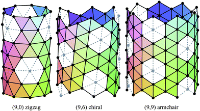
The carbon nanotubes considered here are assumed to be formed by sp2 hybridization3 and the nanotube structure is assumed to comprise hexagonal lattices as shown in Fig. 1. Silicon prefers sp3 bond formation55,60,61 and it is predicted that the four-coordinated atoms form a skewed rhomboid lattice55,60,61 as shown in Fig. 2. The boron nanotubes considered here are assumed to be formed by sp2 hybridization and π-bonds62–67 The lattice structures for boron nanotubes that have been proposed include flat equilateral triangles,40,41,62,71,77–81 puckered equilateral triangles63–65,71,72,81–83 and a novel lattice pattern66 that is a triangular lattice structure with 1/9 hexagonal holes, a structure which is believed to be energetically more stable than a pure triangular lattice.73 However, analysis of the raw data of Yang73,74 reveals a far more complex structure and the model of Yang74 involves three distinct radii; three-quarters of the atoms have an hexagonal based radius, one-eighth have a puckered outer radius and one-eighth have a puckered inner radius. However, although we acknowledge that the polymorphism of boron nanotubes is an important consideration with a number of possible structures which may be more stable than a homogeneous triangular lattice,66 here for simplicity we consider the lattice for boron nanotubes to comprise only equilateral triangles with vertices which are all equidistant from a common axis. As a result, the nanotube lattice assumed here comprises a flat triangular pattern62–67 as shown in Fig. 3. Boron nitride nanotubes have a complex electronic structure such that boron atoms are formed by sp2 hybridization and nitrogen atoms are formed by the unhybridized s and p orbitals.59 Accordingly, the boron nitride nanotube structure is similar to the carbon nanotube but it has two distinct radii.59Fig. 1, 2 and 3 show the general polyhedral model and the atoms are represented by black dots and the bonds between atoms are indicated by black lines. Fig. 4 is the ideal polyhedral model for boron nitride nanotubes and the boron atoms and nitride atoms are represented by solid dots and hollow dots, respectively, and the black lines indicate the bonds. In Fig. 1 and 4 the gray lines represent the conceptual division of each hexagon into four triangles.
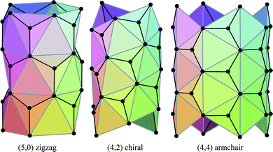 | ||
| Fig. 1 General polyhedral model for carbon nanotubes for zigzag, chiral and armchair tubes. | ||
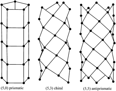 | ||
| Fig. 2 General polyhedral model for silicon nanotubes for prismatic, chiral and antiprismatic tubes. | ||
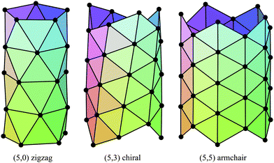 | ||
| Fig. 3 General polyhedral model for boron nanotubes for zigzag, chiral and armchair tubes. | ||
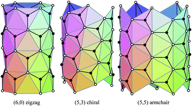 | ||
| Fig. 4 Ideal polyhedral model for boron nitride nanotubes for zigzag, chiral and armchair tubes. | ||
In the follow sections, we present the traditional rolled-up model, the rolled-up model with distinct bond lengths, the ideal polyhedral model and the general polyhedral model for carbon nanotubes (section 2), silicon nanotubes (section 3) and boron nanotubes (section 4). The traditional rolled-up model and the ideal polyhedral model for boron nitride nanotubes are presented in section 5. In section 6, the nanotube radius is discussed and some concluding remarks are made. Throughout this paper we use the subscripts re, pe, rd and pd to designate respectively quantities associated with rolled-up model with equal bond lengths, polyhedral model with equal bond lengths, rolled-up model with distinct bond lengths and polyhedral model with distinct bond lengths.
2 Carbon nanotubes
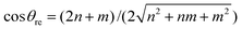
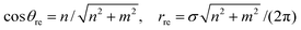
The traditional rolled-up model for carbon nanotubes assumes that all bond lengths and all bond angles are equal and the nanotube can be envisaged as a two dimensional sheet which is rolled into a seamless right circular cylinder.37–39 Carbon nanotubes are categorized into three types, namely zigzag, armchair and chiral, based on the values of the chiral vector Ch = na1 + ma2 where n and m are non-negative integer chiral vector numbers, a1 and a2 are basis vectors and the naming of the nanotubes is indicated by the chiral vector numbers (n, m). Carbon nanotubes are termed zigzag when m = 0 and armchair when m = n. In all other cases, when 0 < m < n they are termed chiral nanotubes.The traditional chiral angle is the angle between the chiral vector Ch and the basis vector a1. The chiral angle for the traditional rolled-up model is given by
 | (1) |
 | (2) |
Experimental results49–54 show that the bond lengths of the nanotubes vary depending on the bond direction because the bond lengths and the bond angles may vary with nanotube curvature.49 The bonds paralleled to the nanotube axis, are found to be shorter than the bonds around the nanotube circumference.49–53 Therefore, from symmetric considerations zigzag and armchair tubes can have two distinct bond lengths and bond angles, while chiral tubes can have three different bond lengths and bond angles.49–54,57
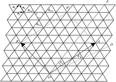
The general rolled-up model must accommodate three different bond lengths57 and thus requires three basis vectors a1, a2 and a3, as shown in Fig. 5. Employing the same notion as the traditional rolled-up model, the two dimensional sheet with distinct bond lengths is rolled along the chiral vector which is still given by Ch = na1 + ma2, but the lengths and direction of the basis vectors may be different from the traditional rolled-up model.
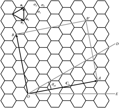 | ||
| Fig. 5 Carbon nanotube constructed from two dimensional sheet with distinct bond lengths. | ||
Since there are three different bond lengths, the nanotubes may have three different bond angles in the plane but the rolled-up model with distinct bond lengths and distinct bond angles could restructure into many different hexagonal patterns such that the sum of the bond angles is less than 2π.50–52,54 The three different bond angles all asymptote to a sum of 2π in the limit as n becomes large50–52 and therefore for the rolled-up model we assume that the three bond angles are equal ϕre = 2π/3.
In Fig. 5, the origin O is located at an arbitrary lattice point. The chiral vector Ch goes from O to A. The sheet is rolled so that the point A coincides with the origin O and the point B coincides with the point B′. When m = 0, which is equivalent to rolling up the nanotube in the direction of OE, the carbon nanotubes is called zigzag. When m = n, which is equivalent to rolling the nanotube in the direction of OD, the resulting to be termed armchair. In all other cases, when 0 < m < n they are termed chiral.
The chiral angle for the general rolled-up models bases on the different bond lengths and given by
 | (3) |
 ,
,  and
and 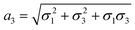 . We note that throughout we use the subscript rd for the rolled-up model with distinct bond lengths. For the special case (m = 0), the chiral angle θrd is zero.
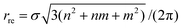
The nanotube radius for the general rolled-up model is given by
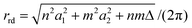 | (4) |
The conventional rolled-up model37–39 and the general rolled-up model,57 all assume that a flat sheet of graphene is rolled into a seamless right circular cylinder. However, a real nanotube has a curvature49 and recently, Cox and Hill44,45 propose a new ideal geometric polyhedral model of single-walled carbon nanotubes, in which all bond lengths are assumed to be equal but the curvature is properly accommodated. This model makes very accurate predictions on the geometric parameters of the nanotube which are in excellent agreement with certain first-principles calculations.68–70
The ideal polyhedral model is based on three fundamental postulates:44,45 (i) all bond lengths are equal σ; (ii) all the adjacent bond angles are equal ϕpe; and (iii) all atomic nuclei are equidistant from a common axis rpe. We note that throughout we use the subscript pe for the polyhedral model with equal bond lengths. For carbon nanotubes, each component of the hexagonal lattice is divided into three isosceles triangles and one equilateral triangle.44,45 The equilateral triangular pattern is shown in Fig. 1 by gray lines and the dots denote the atomic location on each of the isosceles triangles making up a pyramid.
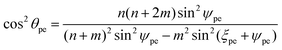
A fundamental parameter for the ideal polyhedral model is the subtend semi-angle ψpe which is the semi-angle subtended at the nanotube axis in the xy-plane of one edge of a equilateral triangle from the lattice. This angle is a root of the following transcendental equation:
| (n2 − m2) sin2(ξpe + ψpe) − n(n + 2m) sin2ξpe + m(2n + m) sin2ψpe = 0 | (5) |
| π/(n + m) ≤ ψpe ≤ π/n | (6) |
While no explicit equation is know for ψpe, an accurate numerical value for the root of the transcendental eqn (5) may be determined after a small number of iterations of Newton's method, using the initial estimate
| ψ0pe = π(2n + m)/[2(n2 + nm + m2)] | (7) |
The chiral angle θpe for the ideal polyhedral model, by which we mean ΔQPQ′, may be derived from the two triangles, ΔPQQ′ and ΔPCQ′ as shown in Fig. 6. The point Q′ defines as the point determined by projecting Q into the xy-plane. The length of PQ is the length of the basis vector a1 and the lengths of CP and CQ′ are the radii rpe. The chiral angle is given by
 | (8) |
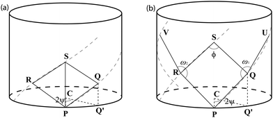 | ||
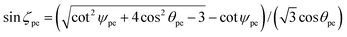
| Fig. 6 Points lying on some helices in three dimensional space for (a) CNTs/BNTs/BNNTs and for (b) SiNTs. | ||
For certain special cases, the chiral angle has two simple exact values. The chiral angle θpe is zero for zigzag tubes (m = 0), and takes the value π/6 for armchair tubes (m = n).
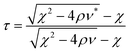
The adjacent bond angle ϕpe is defined as the angle between two bonds when the atoms that are being bonded comprise a single lattice. We need to introduce a new parameter to provide an equation for the adjacent bond angle, since it includes a new parameter which is the angle of incline ζpe of the pyramidal components of the surfaces. The incline angle ζpe is given by
 | (9) |
| cos ϕpe = (– 2 + k2)/(4 + k2) | (10) |
 | (11) |
The nanotube radius for the ideal polyhedral model is given by
| rpe = [σ sin(ϕpe/2) cos θpe]/sin ψpe | (12) |
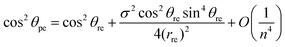
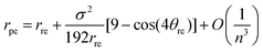
Using the asymptotic expansions method, the chiral angle θpe for the ideal polyhedral model may be written in terms of the traditional chiral angle θre and the traditional nanotube radius rre and is given by
 | (13) |
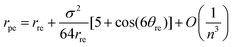 | (14) |
By examining the asymptotic expansions of the equations for the ideal polyhedral model for the chiral angle (8) and the nanotube radius (12) we observe from eqn (13) and (14) that the leading order term of the analytical expressions gives the traditional formulae for rolled-up model (1) and (2) as their leading order term and the next term may be viewed as a first-order correction to the traditional model. This demonstrates that the ideal polyhedral model converges to the traditional rolled-up model for large n.
Table 1 compares the traditional rolled-up model, the ideal polyhedral model and the simulation results Cabria et al.,68 and shows that the results of the ideal polyhedral model are in good agreement with those from the simulation results. The traditional rolled-up model is only close to the simulation results for large values of the nanotube radius. However, the ideal polyhedral model provides much closer results to these from simulation than the traditional rolled-up model.
| (n, m) | r re/Å | r pe/Å | r */Å |
|---|---|---|---|
| (4,0) | 1.5878 | 1.7125 | 1.71 |
| (3,2) | 1.7303 | 1.8109 | 1.80 |
| (4,1) | 1.8191 | 1.9178 | 1.91 |
| (5,0) | 1.9848 | 2.0840 | 2.06 |
| (3,3) | 2.0626 | 2.1258 | 2.12 |
| (4,2) | 2.1005 | 2.1724 | 2.17 |
| (5,1) | 2.2102 | 2.2934 | 2.28 |
| (6,0) | 2.3817 | 2.4641 | 2.45 |
| (4,3) | 2.4146 | 2.4703 | 2.46 |
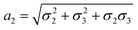
The ideal polyhedral model, which assumes all bond lengths are equal, may be extended to having distinct bond lengths to give the general polyhedral model. The general polyhedral model is similar to the ideal polyhedral model in that it is also based on certain postulates. For carbon nanotubes there are two general polyhedral models, (Model I) and (Model II). Model I is the polyhedral model with distinct bond lengths and distinct bond angles. Model II is the polyhedral model with distinct bond lengths but equal bond angles. In other words, the difference between the two carbon models is the values of the bond angles. Model I assumes three prescribed distinct bond angles but Model II assumes that all the bond angles are the same. In Model I, the bond angles cannot be determined from the bond lengths, and therefore the bond lengths and bond angles must be prescribed. Without prescribed bond angles the general polyhedral model for Model I is not fully determined, and therefore to model nanotubes with the bond angles are not known we have developed the general polyhedral Model II.
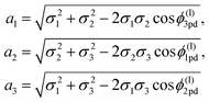
The general polyhedral model for carbon nanotubes (Model I)57 is based on two fundamental postulates: (i) corresponding bonds lying on the same helix are equal in length, either σ1, σ2 or σ3 which are assumed generally to be distinct; and (ii) all atomic nuclei are equidistant rpd from a common axis. For Model II,57 there are three fundamental postulates: (i) corresponding bonds lying on the same helix are equal in length to either σ1, σ2 or σ3 which are assumed generally to be distinct; (ii) all adjacent bond angles are equal to ϕpd; and (iii) all atomic nuclei are equidistant rpd from a common axis. We note that throughout we use the subscript pd for the polyhedral model with distinct bond lengths. We use the superscripts (I) and (II) for models I and II, respectively.
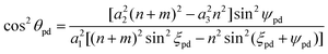
The leading parameter for both models is the subtend semi-angle ψpd which is determined as a root of the following transcendental equations:
| [a22(n + m)2 − a32n2] sin2ψpd + [a32m2 − a12(n + m)2] sin2ξpd + (a12n2 − a22m2) sin2(ξpd + ψpd) = 0 | (15) |
 | (16) |
| ψ0pd = [π(2na21 + mΔ)]/[2(n2a21 + m2a22 + nmΔ)] | (17) |
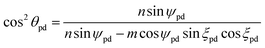
The chiral angle for both Models I and II is given by
 | (18) |
| rpd = a1 cos θpd/(2 sin ψpd) | (19) |
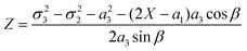
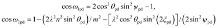
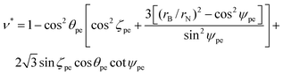
The subtend semi-angle ψ(II)pd and the bond angle ϕ(II)pd for Model II both appear in the transcendental eqn (15), and therefore the angles cannot be determined and we need further constraints. For the ideal polyhedral model, we need to determine the incline angle parameter ζpe by considering the pyramidal components of the surfaces and through the properties of the pyramid and the nanotube radius, we obtain the three unknowns ψ(II)pd, ϕ(II)pd and ζ(II)pd in two equations which are given by
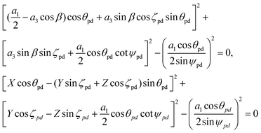 | (20) |
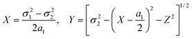
and cos β = (a12 + a32 − a22)/(2a1a3).
For eqn (15) and (20), it is not easy to determine simple strict inequalities on the variables. However, we have found that accurate numerical values can be determined using MAPLE and restricting the angles to the following ranges:
| 0 ≤ ψ(II)pd ≤ π/n, 5π/9 ≤ ϕ(II)pd ≤ 2π/3, − π/4 ≤ ζ(II)pd ≤ π/4 | (21) |
Using the method of asymptotic expansions, the chiral angle θpd is given by
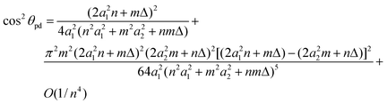 | (22) |
Similarly, the nanotube radius may be rewritten as
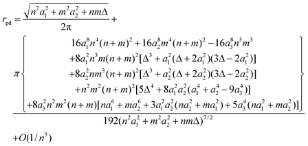 | (23) |
By an examination of these asymptotic expansions for the general polyhedral model for the chiral angle θpd(22) and for the nanotube radius rpd(23), we observe that the leading order terms coincide exactly with the general rolled-up model eqn (3) and (4) and we view the second terms as first-order corrections to the general rolled-up model.
In Table 2, the values of the various bond lengths and bond angles for carbon nanotubes are provided from Table 1 of Jiang et al.51 and compared with the general polyhedral model for Model I. The values of the carbon bond lengths for Table 3 are provided from Table 1 of Budyka et al.,49 while the bond angle values are not given. Accordingly, we use the bond angle arising from the general polyhedral model with distinct bond lengths and the same bond angle and the general polyhedral model for carbon nanotubes for Model II, in order to compare with Budyka et al.49Tables 2 and 3 show that the results of the general polyhedral model to be in excellent agreement with the first-principle simulations.
| (n, m) | σ 1/Å | σ 2/Å | σ 3/Å | ϕ (I)1pd (°) | ϕ (I)2pd (°) | ϕ (I)2pd (°) | r (I) pd/Å | θ (I) pd (°) | r rd/Å | r */Å | θ * (°) |
|---|---|---|---|---|---|---|---|---|---|---|---|
| (5,0) | 1.4669 | 1.4669 | 1.4542 | 118.99 | 118.99 | 112.59 | 2.0761 | 0.000 | 2.0219 | 2.0761 | 0.000 |
| (7,0) | 1.4586 | 1.4586 | 1.4528 | 119.40 | 119.40 | 116.28 | 2.8553 | 0.000 | 2.8146 | 2.8552 | 0.000 |
| (10,0) | 1.4544 | 1.4544 | 1.4518 | 119.69 | 119.69 | 118.20 | 4.0385 | 0.000 | 4.0093 | 4.0386 | 0.000 |
| (20,0) | 1.4516 | 1.4516 | 1.4510 | 119.92 | 119.92 | 119.55 | 8.0178 | 0.000 | 8.0031 | 8.0180 | 0.000 |
| (30,0) | 1.4511 | 1.4511 | 1.4508 | 119.96 | 119.96 | 119.80 | 12.0103 | 0.000 | 12.0005 | 12.0150 | 0.000 |
| (4,2) | 1.4603 | 1.4675 | 1.4555 | 116.92 | 120.59 | 114.19 | 2.1678 | 19.650 | 2.1364 | 2.1678 | 18.702 |
| (6,2) | 1.4564 | 1.4592 | 1.4531 | 118.61 | 120.07 | 116.72 | 2.9284 | 14.074 | 2.8983 | 2.9284 | 13.673 |
| (9,3) | 1.4532 | 1.4544 | 1.4518 | 119.36 | 120.02 | 118.56 | 4.3557 | 13.972 | 4.3351 | 4.3556 | 13.794 |
| (16,6) | 1.4514 | 1.4518 | 1.4510 | 119.79 | 120.01 | 119.57 | 7.8929 | 15.320 | 7.8823 | 7.8930 | 15.262 |
| (25,9) | 1.4510 | 1.4511 | 1.4508 | 119.91 | 120.00 | 119.82 | 12.2120 | 14.810 | 12.2050 | 12.2125 | 14.786 |
| (4,4) | 1.4548 | 1.4604 | 1.4548 | 117.31 | 120.45 | 117.31 | 2.8036 | 30.476 | 2.7856 | 2.8036 | 29.833 |
| (5,5) | 1.4533 | 1.4568 | 1.4533 | 118.27 | 120.26 | 118.27 | 3.4897 | 30.299 | 3.4751 | 3.4899 | 29.887 |
| (6,6) | 1.4525 | 1.4549 | 1.4525 | 118.80 | 120.17 | 118.80 | 4.1782 | 30.204 | 4.1657 | 4.1782 | 29.919 |
| (12,12) | 1.4511 | 1.4517 | 1.4511 | 119.70 | 120.04 | 119.70 | 8.3229 | 30.050 | 8.3165 | 8.3230 | 29.979 |
| (18,18) | 1.4509 | 1.4511 | 1.4509 | 119.87 | 120.02 | 119.87 | 12.4752 | 30.023 | 12.4707 | 12.4750 | 29.991 |
| (n, m) | σ 1/Å | σ 2/Å | σ 3/Å | ϕ (II)pd (°) | θ (II)pd (°) | r (II)pd/Å | r rd/Å | r */Å | Method used in49 |
|---|---|---|---|---|---|---|---|---|---|
| (4,4) | 1.424 | 1.429 | 1.424 | 118.285 | 29.942 | 2.773 | 2.726 | 2.759 | PM3 |
| (4,4) | 1.437 | 1.442 | 1.437 | 118.285 | 29.943 | 2.798 | 2.751 | 2.786 | PBEPBE/3-21C* |
| (4,4) | 1.435 | 1.439 | 1.435 | 118.285 | 29.954 | 2.793 | 2.746 | 2.783 | PBEPBE/6-31C* |
| (4,4) | 1.432 | 1.435 | 1.432 | 118.285 | 29.965 | 2.786 | 2.739 | 2.773 | PBEPBE/6-311C* |
| (4,4) | 1.432 | 1.439 | 1.432 | 118.285 | 29.919 | 2.791 | 2.744 | 2.773 | B3LYP/6-31G |
| (4,4) | 1.429 | 1.435 | 1.429 | 118.285 | 29.931 | 2.784 | 2.737 | 2.773 | B3LYP/3-21G* |
| (5,5) | 1.423 | 1.426 | 1.423 | 118.906 | 29.965 | 3.439 | 3.402 | 3.427 | PM3 |
| (5,5) | 1.420 | 1.425 | 1.420 | 118.906 | 29.942 | 3.435 | 3.398 | 3.421 | PM5 |
| (5,5) | 1.435 | 1.438 | 1.435 | 118.906 | 29.965 | 3.468 | 3.431 | 3.381 | PBEPBE/3-21G* |
| (5,5) | 1.428 | 1.431 | 1.428 | 118.906 | 29.965 | 3.451 | 3.414 | 3.422 | B3LYP/3-21G* |
| (6,6) | 1.422 | 1.424 | 1.422 | 119.241 | 29.977 | 4.109 | 4.078 | 4.099 | PM3 |
| (8,8) | 1.421 | 1.423 | 1.421 | 119.574 | 29.977 | 5.456 | 5.433 | 5.448 | PM3 |
| (9,9) | 1.420 | 1.423 | 1.420 | 119.664 | 29.965 | 6.131 | 6.111 | 6.123 | PM3 |
| (10,10) | 1.420 | 1.422 | 1.420 | 119.728 | 29.977 | 6.805 | 6.786 | 6.799 | PM3 |
| (10,10) | 1.433 | 1.434 | 1.433 | 119.728 | 29.988 | 6.864 | 6.845 | 6.859 | PBEPBE/3-21G* |
| (12,12) | 1.420 | 1.422 | 1.420 | 119.811 | 29.977 | 8.159 | 8.144 | 8.153 | PM3 |
| (15,15) | 1.420 | 1.422 | 1.420 | 119.879 | 29.977 | 10.192 | 10.180 | 10.184 | PM3 |
3 Silicon nanotubes
The nanotube lattice for silicon nanotubes is assumed to comprise only skewed rhombi. The traditional rolled-up model for silicon nanotubes is similar to that for carbon nanotubes in that it assumes that all bond lengths and all bond angles are equal. An extension of the traditional rolled-up model might be described as the general rolled-up model which assumes two distinct bond lengths and that all bond angles are equal. The chiral vector Ch for both models is Ch = na1 + ma2 where the two basis vectors are a1 and a2. The lengths of the basis vectors for the traditional rolled-up model are a1 = a2 = σ where σ is bond length. However, the general rolled-up model may have different bond lengths and a1 = σ1 and a2 = σ2 where σ1 and σ2 are distinct. Fig. 7 shows the general rolled-up model initially drawn on a two dimensional sheet. The terminology for silicon nanotubes is different to that of carbon nanotubes because of the different lattice structure.46,56 When m = 0, which is equivalent to rolling up the nanotube in the direction of OE, we term the nanotubes prismatic because the tube comprises regular n-gon prisms. When m = n, we term the tube antiprismatic which occurs when the sheet is rolled following the direction OD. In all other cases 0 < m < n, the nanotube is termed as chiral.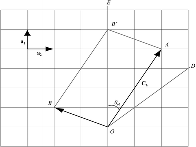 | ||
| Fig. 7 Silicon nanotube constructed from rolling-up a two dimensional sheet with distinct bond lengths. | ||
The main equations for the traditional rolled-up model are given by
 | (24) |
while for the general rolled-up model we have
 | (25) |
For m = 0, the chiral angles θre and θrd are zero. In the case m = n, the chiral angle θre for the traditional rolled-up model is π/4 and the chiral angle θrd for the general model is  which we observe depends upon the bond lengths only. The adjacent bond angle is π/2 for the traditional rolled-up model ϕre and the general rolled-up model ϕrd. Eqn (25) show that when the bond lengths are equal (σ1 = σ2), these equations coincide with eqn (24), and therefore the traditional rolled-up model is a special case of the general rolled-up model.
The ideal polyhedral model is based on three fundamental postulates46 that: (i) all bond lengths are equal to σ; (ii) all the adjacent bond angles are equal to ϕpe; and (iii) all atomic nuclei are equidistant from a common axis rpe. In this event, the subtend semi-angle is determined as a root of the following transcendental equation:
| n tan ξpe + m tan ψpe = 0 | (26) |
The chiral angle can be shown to be given by
 | (27) |
| cos ϕpe = (m2 sin2ψpe)/(n2 cos2ψpe + m2), |
so that the adjacent bond angle ϕpe for the prismatic tube has the constant value π/2. The value of the adjacent bond angle ϕpe for chiral and antiprismatic tubes asymptotes to π/2 in the limit as n becomes large, since the surface of the nanotube approaches a flat plane in this limit. The nanotube radius can be shown to be given by
| rpe = (σ cos θpe)/(2 sin ψpe) | (28) |
The chiral angle θpe and the nanotube radius rpe may be written in terms of the traditional chiral angle θre and the traditional nanotube radius rre by using the method of asymptotic expansions to yield
 | (29) |
 | (30) |
Eqn (29) and (30) show that the leading order terms of the analytical expressions give the traditional formulae (24) as their highest order terms and the second terms provide first-order corrections to the traditional model.
Table 4 compares the nanotube radii for the traditional rolled-up model, the ideal polyhedral model and the simulation results, and show that the results of the ideal polyhedral model are in good agreement with the simulation results of Li et al.,61 who examine a number of prismatic silicon nanotubes using an empirical full-potential linear-muffin-tin-orbital molecular dynamics method. Their silicon nanorings and nanotubes are prismatic silicon nanotubes with atoms at the surface, and their nanotubes are similar to the prismatic nanotubes described here.
| (n, m) | r re/Å | r pe/Å | r */Å |
|---|---|---|---|
| (6,0) | 2.201 | 2.305 | 2.35 |
| (8,0) | 2.935 | 3.012 | 3.00 |
| (10,0) | 3.669 | 3.730 | 3.75 |
For the general polyhedral model, we employ the following three fundamental postulates:56 (i) corresponding bonds lying on the same helix are equal in length to either σ1 or σ2 which are assumed generally to be distinct; (ii) all adjacent bond angles are equal to ϕpd; and (iii) all atomic nuclei are equidistant rpd from a common axis. It may be shown that the subtend semi-angle ψpd for the general polyhedral model is determined as a root of the following transcendental equation:
| 4nm(σ22 sin2ψpd − σ21 sin2ξpd) + (σ21n2 − σ22m2)[sin2(ξpd + ψpd) − sin2(ξpd − ψpd)] = 0, |
 | (31) |
The adjacent bond angle ϕpd is defined as the angle between two bonds where the atoms that are being bonded form part of the same rhombus in the nanotube lattice while the opposite bond angle is the angle between two bonds where the atoms that are being bonded do not form part of the same rhombus in the nanotube lattice. The adjacent bond angle ϕpd is given by
| cos ϕpd = [(λ2 + 1)m2 sin2ψpd − λ2m2 cos2θpd sin2(ξpd + ψpd) − λ2(n + m)2 sin2θpd sin2ψpd]/(2λm2 sin2ψpd) | (32) |
 | (33) |
Table 5 shows a comparison of the silicon nanotube radius for the general polyhedral model and the general rolled-up model as compared with the molecular dynamics simulations at 100 K. We have relaxed the idealised silicon nanotube structures with all the bond lengths set equal to 2.35 Å using the LAMMPS software (see Lee et al.46 and Plimpton75) and we model the silicon pairwise interactions using a Stillinger–Weber potential.76 The σ1*, σ2* and r* are the molecular dynamics simulations results. The numerical data of the structures considered here shows them to be at least metastable in these simulations, the structures obtained from the molecular dynamics simulations for (4, 0), (4, 1) and (4, 2) are shown in Fig. 8, 9 and 10, respectively.
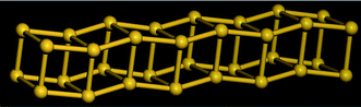 | ||
| Fig. 8 Molecular dynamics result for SiNT (4, 0) at 100 K. | ||
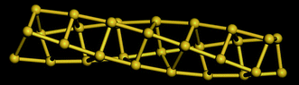 | ||
| Fig. 9 Molecular dynamics result for SiNT (4, 1) at 100 K. | ||
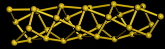 | ||
| Fig. 10 Molecular dynamics result for SiNT (4, 2) at 100 K. | ||
| (n, m) | σ 1*/Å | σ 2*/Å | r*/Å | r pd/Å | r rd/Å |
|---|---|---|---|---|---|
| (4,0) | 2.462 ± 0.031 | 2.573 ± 0.040 | 1.74 ± 0.08 | 1.74 | 1.57 |
| (4,1) | 2.431 ± 0.032 | 2.588 ± 0.017 | 1.75 ± 0.07 | 1.78 | 1.60 |
| (4,2) | 2.479 ± 0.023 | 2.611 ± 0.040 | 1.88 ± 0.03 | 1.96 | 1.78 |
| (5,0) | 2.418 ± 0.051 | 2.574 ± 0.038 | 2.12 ± 0.01 | 2.06 | 1.92 |
| (5,1) | 2.413 ± 0.012 | 2.571 ± 0.021 | 2.07 ± 0.05 | 2.10 | 1.96 |
| (6,0) | 2.429 ± 0.066 | 2.580 ± 0.087 | 2.42 ± 0.07 | 2.43 | 2.32 |
| (6,1) | 2.449 ± 0.055 | 2.564 ± 0.076 | 2.47 ± 0.45 | 2.49 | 2.37 |
| (7,0) | 2.466 ± 0.098 | 2.571 ± 0.091 | 2.84 ± 0.69 | 2.84 | 2.75 |
| (7,1) | 2.447 ± 0.037 | 2.602 ± 0.028 | 2.83 ± 0.43 | 2.85 | 2.76 |
Table 6 shows the bond angles for the polyhedral model with distinct bond lengths compared with these obtained from the molecular dynamics simulations at 100 K. The bond angles ϕ*, ω1* and ω2* are the average of the bond angles measured from two rings of the nanotube and the error is two standard deviations. The bond angles ϕpd, ω1pd and ω2pd are calculated from the polyhedral model using the values σ1* and σ2* from Table 5. The results of the adjacent bond angle ϕpd and the opposite bond angle ω1pd of the polyhedral model and the molecular dynamics simulations are in excellent agreement. The calculated adjacent bond angle ϕ* has a large error, and therefore we have grouped the raw data into two groups as either above or below π/2 which are termed the adjacent bond angles ϕa* and ϕb*. The low value of the error obtained for the adjacent bond angles ϕa* and ϕb* suggests that the adjacent bond angle may have two distinct values. The opposite bond angle ω2pd for prismatic tubes does not match well with the molecular dynamics simulations results because the tubes possess an off-centred structure which alternates along the nanotube length as shown in Fig. 8. The structures of the molecular dynamics simulations results for (4,1) and (4,2), which are shown in Fig. 9 and 10, are similar to those predicted by the general polyhedral model. However, Table 5 shows that the results of the general polyhedral model are in excellent agreement with the molecular dynamics simulations.
| (n, m) | ϕ* (°) | ϕ a* (°) | ϕ b* (°) | ω 1* (°) | ω 2* (°) | ϕ pd (°) | ω 1pd (°) | ω 2pd (°) |
|---|---|---|---|---|---|---|---|---|
| (4,0) | 90.13 ± 15.69 | 82.57 ± 1.72 | 97.68 ± 1.34 | 90.00 ± 5.21 | 158.08 ± 2.40 | 90.00 | 90.00 | 180.00 |
| (4,1) | 88.49 ± 10.82 | 83.27 ± 0.87 | 93.71 ± 0.99 | 98.63 ± 0.56 | 174.79 ± 1.34 | 86.98 | 100.27 | 170.59 |
| (4,2) | 85.58 ± 12.83 | 79.39 ± 0.97 | 91.78 ± 1.01 | 118.03 ± 1.31 | 162.86 ± 3.04 | 84.34 | 119.02 | 157.60 |
| (5,0) | 89.99 ± 12.08 | 84.70 ± 5.30 | 95.29 ± 5.54 | 107.99 ± 2.15 | 162.30 ± 2.04 | 90.00 | 108.00 | 180.00 |
| (5,1) | 89.40 ± 8.37 | 85.37 ± 1.18 | 93.44 ± 1.29 | 112.12 ± 1.08 | 178.13 ± 1.20 | 88.79 | 113.19 | 175.61 |
| (6,0) | 89.98 ± 13.58 | 83.94 ± 5.69 | 96.02 ± 5.90 | 119.94 ± 4.90 | 160.33 ± 4.69 | 90.00 | 120.00 | 180.00 |
| (6,1) | 89.46 ± 14.81 | 82.49 ± 4.85 | 96.43 ± 3.41 | 112.43 ± 11.90 | 158.94 ± 8.96 | 89.46 | 122.87 | 177.73 |
| (7,0) | 89.93 ± 18.04 | 81.59 ± 5.65 | 98.26 ± 6.67 | 128.39 ± 10.76 | 152.97 ± 8.32 | 90.00 | 128.57 | 180.00 |
| (7,1) | 89.52 ± 12.95 | 83.68 ± 5.42 | 95.36 ± 5.03 | 130.32 ± 8.49 | 160.01 ± 7.15 | 89.70 | 130.41 | 178.57 |
4 Boron nanotubes
The traditional rolled-up model40,41 assumes that the lattice pattern of a boron nanotube comprises flat equilateral triangles and that all bond lengths and all bond angles are equal. The terminology for boron nanotubes is precisely the same as that used for carbon nanotubes with zigzag tubes where m = 0, armchair where m = n and chiral where 0 < m < n. The chiral angle θre coincides with that for carbon nanotubes (1) but the radius rre is different and is given by
In generalising this model, Lee et al.47 have proposed a rolled-up model with distinct bond lengths. Since there are three different bond lengths, the nanotubes will have three different adjacent bond angles, which are defined as the angle between two of the bonds where the atoms that are being bonded comprise a single triangle in the nanotube lattice. There are three adjacent bond angles ϕ1rd, ϕ2rd and ϕ3rd, which are shown in Fig. 11, and are given by
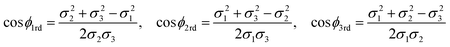 | (34) |
 | ||
| Fig. 11 Boron nanotube constructed from two dimensional sheet with distinct bond lengths. | ||
The ideal polyhedral model is based on the two fundamental postulates47 that: (i) all bond lengths are equal σ; and (ii) all atomic nuclei are equidistant from a common axis rpe. The number of fundamental postulates for boron nanotubes are fewer than is the case for carbon nanotubes and silicon nanotubes because the adjacent bond angle ϕpe = π/3 for the boron nanotubes may be derived immediately from postulate (i) trivially, and therefore an independent adjacent bond angle is not postulated.47
The basis vectors and the pattern for boron nanotubes are the same as for the ideal polyhedral model for carbon nanotubes with each hexagon divided into six equilateral triangles,44,45 and therefore only equilateral triangles need be considered for boron nanotubes.47Fig. 1 shows that the equilateral triangles pattern by gray lines and without pyramids are the same as in Fig. 3. The length of the basis vectors for boron nanotubes is a1 = a2 = σ. As a result, the equations for the subtend semi-angle ψpe, an initial value for a small number of iterations of Newton's method, the chiral angle θpe and the radius rpe are the same as the ideal polyhedral model for carbon nanotubes, eqn (5), (7), (8) and (12), respectively. Since the adjacent bond angle ϕpe for boron nanotubes is π/3 therefore the radius rpe might be simplified to rpe = (σ cos θpe)/(2 sin ψpe). Table 7 shows that the results of the ideal polyhedral model are in good agreement with local density simulation results.
| (n, m) | σ/Å | r re/Å | r pe/Å | r*/Å |
|---|---|---|---|---|
| (12,0) | 1.72 | 3.285 | 3.323 | 3.35 |
| (15,0) | 1.71 | 4.082 | 4.112 | 4.12 |
The general polyhedral model for boron nanotubes58 is also based on two fundamental postulates that: (i) corresponding bonds lying on the same helix are equal in length, either σ1, σ2 or σ3 which are assumed generally to be distinct; and (ii) all atomic nuclei are equidistant rpd from a common axis. Similarly, the equations for the subtend semi-angle ψpd, an initial value for a small number of iterations of Newton's method, the chiral angle θpd and the radius rpd are the same as the general polyhedral model for carbon nanotubes, eqn (15), (17), (18) and (19), respectively. The lengths of the basis vectors for boron nanotubes are a1 = σ1, a2 = σ2 and a3 = σ3.
Fig. 12 shows the general polyhedral model with 1/9 hexagonal holes. In this Figure the missing boron atoms are represented by gray dots and the image bonds between boron atoms and missing atoms are indicated by gray dashed lines. Table 8 compares the general rolled-up model, the general polyhedral model for zigzag and armchair tubes with Yang et al.73 We emphasize that the data shown in the final column of Table 8 arises from Yang et al.73 and Yang74 upon averaging three distinct radii and the comparison is with a different lattice structure involving both triangles and 1/9 missing atoms. In Table 8 we have arbitrarily adopted values of σ1 for zigzag and σ1, σ2 and σ3 for armchair, such that use of our formulae gives an excellent agreement with the results of Yang et al.73 and Yang.74 We comment that since σ2 and σ3 do not appear in the formula for the radius for zigzag, these can adopt any values. We see that on adopting this strategy for both zigzag and armchair nanotubes, the polyhedral model is in excellent agreement with these studies.73,74
 | ||
| Fig. 12 Polyhedral model for boron nanotubes with 1/9 hexagonal holes for zigzag, chiral and armchair tubes. | ||
| (n, m) | σ 1/Å | σ 2/Å | σ 3/Å | r rd/Å | r pd/Å | r */Å |
|---|---|---|---|---|---|---|
| (12,0) | 1.679 | — | — | 3.207 | 3.244 | 3.242 |
| (15,0) | 1.679 | — | — | 3.008 | 4.038 | 4.036 |
| (18,0) | 1.679 | — | — | 4.810 | 4.834 | 4.836 |
| (21,0) | 1.679 | — | — | 5.612 | 5.633 | 5.634 |
| (24,0) | 1.679 | — | — | 6.413 | 6.332 | 6.431 |
| (27,0) | 1.679 | — | — | 7.215 | 7.231 | 7.229 |
| (9,9) | 1.670 | 1.670 | 1.647 | 4.162 | 4.183 | 4.180 |
| (12,12) | 1.670 | 1.670 | 1.647 | 5.549 | 5.565 | 5.568 |
| (15,15) | 1.670 | 1.670 | 1.647 | 6.937 | 6.950 | 6.944 |
| (18,18) | 1.670 | 1.670 | 1.647 | 8.324 | 8.335 | 8.329 |
| (21,21) | 1.670 | 1.670 | 1.647 | 9.712 | 9.721 | 9.736 |
5 Boron nitride nanotubes
Boron nitride nanotubes have a similar structure to that of carbon nanotubes but they have two radii such that all boron atoms have one radius and all nitrogen atoms have another radius.43 As is the case for carbon, the traditional rolled-up model for boron nitride has both atomic spaces located on a flat two dimensional sheet and therefore all the equations of the traditional rolled-up model are the same as those for carbon nanotubes,42 including the chiral angle (1) and the radius (2).Cox and Hill48 propose an ideal polyhedral model for single-walled boron nitride nanotubes that includes the two radii structure. Their ideal polyhedral model has five postulates: (i) all bonds are of equal length σ; (ii) all bond angles ϕB for the boron atoms are equal; (iii) all boron atoms lie at an equal distance rB from the nanotube axis; (iv) all nitrogen atoms lie at an equal distance rN from the nanotube axis; and (v) there exits a fixed ratio of pyramidal height τ between the boron species, compared to the corresponding height in a symmetric single species nanotube. The boron atoms have a flatter structure of bonds which are located closer to the nanotube axis as compared to the nitrogen atoms. If all the bond angles are equal for the nitrogen atoms then the model would be forced to be exactly that for carbon nanotubes when all the bond angles are equal.
The subtend semi-angle ψpe, the chiral angle θpe and the incline angle ζpe for boron nitride nanotubes are the same as those for carbon nanotubes, namely eqn (5), (8) and (9). The adjacent bond angles and the radii are different to carbon nanotubes but the coefficients of the constituent pyramids are the same as those for eqn (11). The adjacent bond angle for boron atoms is
| cos ϕB = (−2 + τ2k2)/(4 + τ2k2) | (35) |
The two radii for boron nitride nanotubes are given by
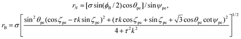 | (36) |
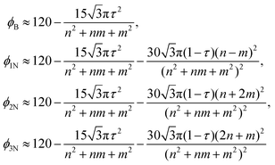 | (37) |
The value for the constant of proportionality τ may be determined by the boron angles,
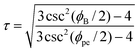 | (38) |
where
In Table 9, the bond angles ϕB* and ϕN* in are found by density functional theory within the generalized-gradient approximation, implemented via the Vienna ab initio Simulation Package (VASP).84 The value of τ is calculated from (38). A comparison of the bond angles shows that the average of nitrogen bond angles are a close match with the results of Barnard et al.84
| (n, m) | ϕ B* (°) | ϕ N* (°) | ϕ (°) | τ |
|---|---|---|---|---|
| (6,6) | 119.75 | 118.48 ± 0.82 | 119.24 | 0.57 ± 0.01 |
| (9,9) | 119.89 | 119.32 ± 0.38 | 119.66 | 0.57 ± 0.03 |
| (12,12) | 119.94 | 119.62 ± 0.21 | 119.81 | 0.56 ± 0.04 |
| (n, m) | ϕ 1N (°) | ϕ 2N (°) | ϕ 3N (°) | ![[small phi, Greek, macron]](https://www.rsc.org/images/entities/char_e0d6.gif) N (°) N (°) |
|---|---|---|---|---|
| (6,6) | 119.75 | 117.86 | 117.86 | 118.49 ± 0.89 |
| (9,9) | 119.89 | 119.04 | 119.04 | 119.32 ± 0.40 |
| (12,12) | 119.94 | 119.45 | 119.45 | 119.61 ± 0.23 |
6 Results and conclusions
For the general rolled-up model the equations for the chiral angle, (3) and (25)1 and for radius (4) and (25)2 are the same as the traditional rolled-up model defined by (1), (2) and (24), when the bond lengths are equal so that the traditional rolled-up model is a special case of the general rolled-up model.56–58 The equations for the general polyhedral model (18), (19) and (31) are also the same as the equations for the ideal polyhedral model (8), (12), (27) and (28) when the bond lengths are equal, and therefore the general polyhedral model includes the ideal polyhedral model.56–58 The traditional rolled-model is a special case of the general rolled-up model and similarly the ideal polyhedral model is a special case of the general polyhedral model.From the asymptotic expansions (13), (14), (29), (30) and (37) for the ideal polyhedral model,44,46–48 the first terms are exactly the traditional rolled-up model eqn (1), (2) and (24) and the second term may be viewed as a first-order correction to the traditional model. Similarly, the first terms of the asymptotic expansions (22), (23), (29) and (30) for the general polyhedral model56–58 are exactly the general rolled-up model eqn (3), (4) and (25) and the second term is a first-order correction to the traditional model. This demonstrates that the polyhedral models converge to the rolled-up models for large n. As a result, the polyhedral models include the rolled-up and ideal models or corresponding general cases, and therefore the general polyhedral model incorporates both rolled-up models and the ideal polyhedral model.
Tables 1, 4 and 7 show that the results of the ideal polyhedral model are in good agreement with those arising from simulation results. For the smaller radii nanotubes, there is a large difference in the radius predicted by the traditional rolled-up model and that arising from the molecular dynamics simulations. This phenomenon is due to the increasing curvature of the tube surface as n becomes small, so that the nanotubes with the smallest values of n have the largest curvature. Tables 2, 3, 5 and 8 show comparisons of the radius from computational studies (molecular dynamics simulations or ab initio) with the results of the general polyhedral model and the general rolled-up model. In almost all cases, the results for the general polyhedral model and the computational studies are in excellent agreement.
In summary, the conventional rolled-up model of nanotubes is an approximate model and completely ignores any effects due to curvature. Accordingly, this opens up the possibility of providing exact geometric constructions which correctly take into account the curvature of the nanotube, but are in complete accord with traditional models for large radii nanotubes. The present paper summarizes the work of the authors which addresses exact nanotube construction based upon certain geometric principles. Polyhedral models are proposed for the four materials, carbon, silicon, boron and boron nitride. In general, the proposed new geometric models are in excellent agreement with existing data from purely numerical approaches and the models can be readily extended to incorporate distinct bond lengths.
| Symbols | Meaning | Equation where first used |
|---|---|---|
| β | Parameter cos β = (a12 + a32 − a22)/(2a1a3) | (20) |
| Δ | Parameter Δ = (a12 + a22 − a32) | (3) |
| ϕ pe | Bond angle for the ideal polyhedral model | (10) |
| ϕ re | Bond angle for the traditional rolled-up model for CNT, SiNT and BNNT | |
| ϕ (I)1pd, ϕ(I)2pd, ϕ(I)2pd | Distinct bond angles for the CNT general polyhedral Model I | (16) |
| ϕ (II)pd | Bond angle for the CNT general polyhedral Model II | (21) |
| ϕ 1rd, ϕ2rd, ϕ3rd | Distinct bond angles for the rolled-up model for BNT | (34) |
| ϕ B | Bond angles for the ideal polyhedral model for boron atoms of BNNT | (35) |
| ϕ 1N, ϕ2N, ϕ3N | Distinct bond angles for the ideal polyhedral model for nitride atoms of BNNT | (37) |
| λ | The ratio of the bond lengths λ = σ1/σ2 | (32) |
| θ re | Chiral angle for the traditional rolled-up model | (1) |
| θ rd | Chiral angle for the general rolled-up model | (3) |
| θ pe | Chiral angle for the ideal polyhedral model | (8) |
| θ pd | Chiral angle for the general polyhedral model | (18) |
| ρ, χ, ν | Parameter | (11) |
| σ | Bond length | (2) |
| σ 1, σ2, σ3 | Distinct bond lengths | (16) |
| τ | A fixed ratio of pyramidal height | (35) |
| ω 1pd, ω2pd | Distinct opposite bond angles for SiNT | (33) |
| ξ | Parameter (nψ − π)/m | (5) |
| ψ pe | Subtend semi-angle for the ideal polyhedral model | (5) |
| ψ pd | Subtend semi-angle for the general polyhedral model | (15) |
| ψ 0pe | Initial value of Newton's method for the ideal polyhedral model | (7) |
| ψ 0pd | Initial value of Newton's method for the general polyhedral model | (17) |
| ζ pe | Incline angle for the ideal polyhedral model | (9) |
| ζ pd | Incline angle for the general polyhedral model | (20) |
| a 1 , a2, a3 | Basis vectors | (3) |
| C h | Chiral vector | |
| k | Parameter k2ρ + kχ + ν = 0 and k is the nondimensional pyramidal height | (10) |
| n, m | Chiral vector numbers | (1) |
| r re | Nanotube radius for the traditional rolled-up model | (2) |
| r rd | Nanotube radius for the general rolled-up model | (4) |
| r pe | Nanotube radius for the ideal polyhedral model | (12) |
| r pd | Nanotube radius for the general polyhedral model | (19) |
| r B | Nanotube radius for boron atoms of the ideal polyhedral model | (36) |
| r N | Nanotube radius for nitride atoms of the ideal polyhedral model | (36) |
| X, Y, Z | Cartesian coordinates for the atomic location at the top of a pyramid | (20) |
Acknowledgements
The support of the Australian Research Council, both through the Discovery Project Scheme and for providing an Australian Professorial Fellowship for JMH and an Australian Post-doctoral Fellowship for BJC is gratefully acknowledged. The authors are also grateful to Dr Xiaobao Yang74 for providing the raw numerical data from Yang et al.73References
- P. V. Kamat and L. M. Liz-marzan, in Nanoscale Materials, 2003, Kluwer Academic Publishers, London Search PubMed.
- B. J. Cox, T. A. Hilder, D. Baowan, N. Thamwattana and J. M. Hill, Int. J. Nanotechnol., 2008, 5, 197–217 Search PubMed.
- S. Iijima, Nature, 1991, 354, 56–8 CrossRef CAS.
- I. Boustani, A. Quandt and P. Kramer, Europhys. Lett., 1996, 36, 583 CrossRef CAS.
- I. Boustani and A. Quandt, Europhys. Lett., 1997, 39, 527 CrossRef CAS.
- D. Ciuparu, R. F. Klie, Y. Zhu and L. Pfefferle, J. Phys. Chem. B, 2004, 108, 3967–9 CrossRef CAS.
- J. Sha, J. Niu, X. Ma, J. Xu, X. Zhang, Q. Yang and D. Yang, Adv. Mater., 2002, 14, 1219 CrossRef CAS.
- P. Castrucci, M. Scarselli, M. D. Crescenzi, M. Diociaiuti, P. S. Chaudiari, C. Balasubramanian, T. M. Bhave and S. V. Bhoraskar, Thin Solid Films, 2006, 508, 226 CrossRef CAS.
- S. Y. Jeong, J. Y. Kim, H. D. Yang, B. N. Yoon, S. H. Choi, H. K. Kang, C. W. Yang and Y. H. Lee, Adv. Mater., 2003, 15, 1172 CrossRef CAS.
- N. G. Chopra, R. J. Luyken, K. Cherrey, V. H. Crespi, M. L. Cohen, S. G. Louie and A. Zettle, Science, 1995, 269, 966 CrossRef CAS.
- R. Ma, Y. Bando and T. Sato, Adv. Mater., 2002, 14, 366 CrossRef CAS.
- T. Laude, Y. Matsui, A. Marraud and B. Jouffrey, Appl. Phys. Lett., 2000, 76, 3239 CrossRef CAS.
- V. V. Pokropivny, V. V. Skorokhod, G. S. Oleinik, A. V. Kurdyumov, T. S. Bartnitskaya, A. V. Pokropivny, A. G. Sisonyuk and D. M. Sheichenko, J. Solid State Chem., 2000, 154, 214 CrossRef CAS.
- W. Han, Y. Bando, K. Kurashima and T. Sato, Appl. Phys. Lett., 1998, 73, 3085 CrossRef CAS.
- K. B. Shelimov and M. Moskovits, Chem. Mater., 2000, 12, 250 CrossRef CAS.
- O. R. Lourie, C. R. Jones, B. M. Bartlett, P. C. Gibbons, R. S. Ruoff and W. E. Buhro, Chem. Mater., 2000, 12, 1808 CrossRef CAS.
- Y. Chen, J. F. Gerald, J. S. Williams and S. Bulcock, Chem. Phys. Lett., 1999, 299, 260 CrossRef CAS.
- A. Rothschild, J. Sloan and R. Tenne, J. Am. Chem. Soc., 2000, 122, 5169–79 CrossRef CAS.
- C. Ye, G. Meng, Z. Jiang, Y. Wang, G. Wang and L. Zhang, J. Am. Chem. Soc., 2002, 124, 15180–1 CrossRef CAS.
- X. P. Shen, G. Yin, W. L. Zhang and Z. Xu, Solid State Commun., 2006, 140, 116–9 CrossRef CAS.
- H. Zhang, S. Zhang, S. Pan, G. Li and J. Hou, Nanotechnology, 2004, 15, 945–8 CrossRef CAS.
- Y. C. Zhu, Y. Bando and Y. Uemura, Chem. Commun., 2003, 836–7 RSC.
- J. Q. Hu, Q. Li, X. M. Meng, C. S. Lee and S. T. Lee, Chem. Mater., 2003, 15, 305 CrossRef CAS.
- Y. J. Xing, Z. H. Xi, Z. Q. Xue, X. D. Zhang, J. H. Song, R. M. Wang, J. Xu, Y. Song, S. L. Zhang and D. P. Yu, Appl. Phys. Lett., 2003, 83, 1689 CrossRef CAS.
- X. H. Zhang, S. Y. Xie, Z. Y. Jiang, X. Zhang, Z. Q. Tian, Z. X. Xie, R. B. Huang and L. S. Zheng, J. Phys. Chem. B, 2003, 107, 10114 CrossRef CAS.
- Ş. Erkoç and H. Kökten, Phys. E., 2005, 28, 162 CrossRef CAS.
- Z. C. Tu and X. Hu, Phys. Rev. B: Condens. Matter Mater. Phys., 2006, 74, 035434 CrossRef.
- S. L. Elizondo and J. W. Mintmire, J. Phys. Chem. C, 2007, 111, 17821 CrossRef CAS.
- J. Goldberger, R. He, Y. Zhang, S. Lee, H. Yan, H. J. Choi and P. Yang, Nature, 2003, 422, 599 CrossRef CAS.
- Q. Wu, Z. Hu, X. Wang, Y. Lu, X. Chen, H. Xu and Y. Chen, J. Am. Chem. Soc., 2003, 125, 10176 CrossRef CAS.
- E. P. A. M. Bakkers and M. A. Verheijen, J. Am. Chem. Soc., 2003, 125, 3440 CrossRef CAS.
- R. Fan, Y. Wu, D. Li, M. Yue, A. Majumdar and P. Yang, J. Am. Chem. Soc., 2003, 125, 5254 CrossRef CAS.
- J. H. Jung, H. Kobayashi, K. J. C. van Bommel, S. Shinkai and T. Shimizu, Chem. Mater., 2002, 14, 1445 CrossRef CAS.
- S. M. Liu, L. M. Gan, L. H. Liu, W. D. Zhang and H. C. Zeng, Chem. Mater., 2002, 14, 1391 CrossRef CAS.
- Z. R. Tian, J. A. Voigt, B. Mckenzie and H. Xu, J. Am. Chem. Soc., 2003, 125, 12384 CrossRef CAS.
- G. Wu, L. Zhang, B. Cheng, T. Xie and X. Yuan, J. Am. Chem. Soc., 2004, 126, 5976–7 CrossRef CAS.
- M. S. Dresselhaus, G. Dresselhaus and R. Saito, Phys. Rev. B: Condens. Matter, 1992, 45, 6234–42 CrossRef CAS.
- M. S. Dresselhaus, G. Dresselhaus and R. Saito, Carbon, 1995, 33, 883–91 CrossRef CAS.
- R. A. Jishi, M. S. Dresselhaus and G. Dresselhaus, Phys. Rev. B: Condens. Matter, 1993, 47, 16671–4 CrossRef CAS.
- A. Gindulyte, W. N. Lipscomb and L. Massa, Inorg. Chem., 1998, 37, 6544–5 CrossRef CAS.
- V. Dadashev, A. Gindulyte, W. N. Lipscomb, L. Massa and R. Squire, Proposed new materials: boron fullerenes, nanotubes and nanotori in Structures and Mechanisms: from Ashes to Enzymes, ed. G. R. Eaton, D. C. Wiley and O. Jardetzky, Oxford University Press, Washington, 2002, Ch. 5, pp. 79–102 Search PubMed.
- A. Rubio, J. L. Corkill and M. L. Cohen, Phys. Rev. B: Condens. Matter, 1994, 49, 5081–4 CrossRef CAS.
- P. Saxena and S. P. Sanyal, Phys. E., 2004, 24, 244–8 CrossRef CAS.
- B. J. Cox and J. M. Hill, Carbon, 2007, 45, 1453–62 CrossRef CAS.
- B. J. Cox and J. M. Hill, Carbon, 2008, 46, 711–3 CrossRef CAS.
- R. K. F. Lee, B. J. Cox and J. M. Hill, J. Phys.: Condens. Matter, 2009, 21, 075301 CrossRef.
- R. K. F. Lee, B. J. Cox and J. M. Hill, J. Phys. A: Math. Theor., 2009, 42, 065204 CrossRef.
- B. J. Cox and J. M. Hill, J. Phys. Chem. C, 2008, 112, 16248–55 CrossRef CAS.
- M. F. Budyka, T. S. Zyubina, A. G. Ryabenko, S. H. Lin and A. M. Mebel, Chem. Phys. Lett., 2005, 407, 266–71 CrossRef CAS.
- J. Kurti, V. Zolyomi, M. Kertesz and G. Sun, New J. Phys., 2003, 5, 125 CrossRef.
- H. Jiang, P. Zhang, B. Liu, Y. Huans, P. H. Geubelle, H. Gao and K. C. Hwang, Comput. Mater. Sci., 2003, 28, 429–42 CrossRef CAS.
- V. K. Jindal and A. N. Imtani, Comput. Mater. Sci., 2008, 44, 156–62 CrossRef CAS.
- P. M. Agrawal, B. S. Sudalayandi, L. M. Raff and R. Komanduri, Comput. Mater. Sci., 2008, 41, 450–6 CrossRef CAS.
- K. Kanamitsu and S. Saito, J. Phys. Soc. Jpn., 2002, 71, 483–6 CrossRef CAS.
- J. Bai, X. C. Zeng, H. Tanaka and J. Y. Zeng, Proc. Natl. Acad. Sci. U. S. A., 2004, 101, 2664–8 CrossRef CAS.
- R. K. F. Lee, B. J. Cox and J. M. Hill, J. Math. Chem., 2010, 47, 569–89 CrossRef CAS.
- R. K. F. Lee, B. J. Cox and J. M. Hill, Fullerenes, Nanotubes and Carbon Nanostructures Search PubMed , accepted.
- R. K. F. Lee, B. J. Cox and J. M. Hill, J. Phys. Chem. C, 2009, 113, 19794–805 CrossRef CAS.
- N. Park, J. Cho and H. Nakamura, J. Phys. Soc. Jpn., 2004, 73, 2469–72 CrossRef CAS.
- X. Wang, Z. Huang, T. Wang, Y. W. Tang and X. C. Zeng, Phys. B, 2008, 403, 2021 CrossRef CAS.
- B. X. Li and P. L. Cao, J. Mol. Struct. (THEOCHEM), 2004, 679, 127 CrossRef CAS.
- B. Kiran, S. Bulusu, H. J. Zhai, S. Yoo, X. C. Zeng and L. S. Wang, Proc. Natl. Acad. Sci. U. S. A., 2005, 102, 961–4 CrossRef CAS.
- J. Kunstmann and A. Quandt, Phys. Rev. B: Condens. Matter Mater. Phys., 2006, 74, 035413 CrossRef.
- I. Boustani, A. Quandt and A. Rubio, J. Solid State Chem., 2000, 154, 269–74 CrossRef CAS.
- M. H. Evans, J. D. Joannopoulos and S. T. Pantelides, Phys. Rev. B: Condens. Matter Mater. Phys., 2005, 72, 045434 CrossRef.
- H. Tang and S. Ismail-Beigi, Phys. Rev. Lett., 2007, 99, 115501 CrossRef.
- K. C. Lau and R. Pandey, J. Phys. Chem. C, 2007, 111, 2906–12 CrossRef CAS.
- I. Cabria, J. W. Mintmire and C. T. White, Phys. Rev. B: Condens. Matter Mater. Phys., 2003, 67, 121406 CrossRef.
- M. Machon, S. Reich, C. Thomsen, D. Sanchez-Portal and P. Ordejon, Phys. Rev. B: Condens. Matter Mater. Phys., 2002, 66, 155410 CrossRef.
- V. N. Popov, New J. Phys., 2004, 6, 17 CrossRef.
- I. Cabria, M. J. Lopez and J. A. Alonso, Nanotechnology, 2006, 17, 778–85 CrossRef CAS.
- I. Cabria, J. A. Alonso and M. J. Lopez, Phys. Status Solidi A, 2006, 203, 1105–10 CrossRef CAS.
- X. Yang, Y. Ding and J. Ni, Phys. Rev. B: Condens. Matter Mater. Phys., 2008, 77, 041402 CrossRef.
- X. Yang, Personal communication.
- S. J. Plimpton, J. Comput. Phys., 1995, 117, 1–19 CrossRef CAS.
- F. H. Stillinger and T. A. Weber, Phys. Rev. B: Condens. Matter, 1985, 31, 5262–71 CrossRef CAS.
- N. G. Szwacki, A. Sadrzadeh and B. I. Yakobson, Phys. Rev. Lett., 2007, 98, 166804 CrossRef.
- I. Boustani and A. Quandt, Comput. Mater. Sci., 1998, 11, 132–7 CrossRef CAS.
- D. L. V. K. Prasad and E. D. Jemmis, J. Mol. Struct. (THEOCHEM), 2006, 771, 111–5 CrossRef CAS.
- I. Boustani, A. Quandt, E. Hernandez and A. Rubio, J. Chem. Phys., 1999, 110, 3176–85 CrossRef CAS.
- J. Kunstmann and A. Quandt, Chem. Phys. Lett., 2005, 402, 21–6 CrossRef CAS.
- A. Quandt, A. Y. Liu and I. Boustani, Phys. Rev. B: Condens. Matter Mater. Phys., 2001, 64, 125422 CrossRef.
- A. Sebetci, E. Mete and I. Boustani, J. Phys. Chem. Solids, 2008, 69, 2004–12 CrossRef CAS.
- A. S. Barnard, I. K. Snook and S. P. Russo, J. Mater. Chem., 2007, 17, 2892–98 RSC.
| This journal is © The Royal Society of Chemistry 2010 |