Co-production of decarbonized synfuels and electricity from coal + biomass with CO₂ capture and storage: an Illinois case study

Abstract

Energy, carbon, and economic performances are estimated for facilities co-producing Fischer–Tropsch Liquid (FTL) fuels and electricity from a co-feed of biomass and coal in Illinois, with capture and storage of by-product CO₂. The estimates include detailed modeling of supply systems for corn stover or mixed prairie grasses (MPG) and of feedstock conversion facilities. Biomass feedstock costs in Illinois (delivered at a rate of one million tonnes per year, dry basis) are $ 3.8/GJ_HHV for corn stover and $ 7.2/GJ_HHV for MPG. Under a strong carbon mitigation policy, the economics of co-producing low-carbon fuels and electricity from a co-feed of biomass and coal in Illinois are promising. An extrapolation to the United States of the results for Illinois suggests that nationally significant amounts of low-carbon fuels and electricity could be produced this way.

---

Broader context

This analysis highlights the merits of making low-carbon liquid fuels thermochemically rather than biochemically by simultaneously: (i) capturing and storing CO₂ from biomass to increase its carbon-mitigation potential; (ii) co-processing biomass with coal to exploit the scale economies of coal conversion, the low cost of coal as a feedstock, and, with CO₂ capture and storage (CCS), the reduced amount of biomass needed to make low-carbon fuels relative to conventional biofuels; and (iii) producing electricity as a major co-product to increase energy conversion efficiency and reduce capital costs relative to separate systems for producing liquid fuels and electricity. It shows the strategic importance of simultaneously pursuing carbon mitigation for transportation fuels and electricity and that the pursuit of carbon mitigation and energy security goals for transportation fuels need not be in conflict. Although the approach involves radically different energy system configurations from systems currently in use, the systems described involve components that are either already commercial or could become commercially available during the next decade. Requirements are: (i) demonstration that CCS is viable as a major carbon mitigation option, (ii) commercialization of large biomass gasifiers, and (iii) commercial-scale demonstrations of co-production systems that co-process coal and biomass with CCS.

1 Introduction

In the United States, interest has been intensifying in recent years in secure domestic alternatives to oil for satisfying transportation energy needs. Moreover, when a carbon mitigation policy is put in place, mitigation strategies will be needed for the transportation sector, which accounts for one-third of US. fossil fuel greenhouse gas (GHG) emissions. Significant energy supply options for meeting these challenges are biomass and coal.

Biomass grown on a sustainable basis can help mitigate climate change because the CO₂ released in its ultimate combustion is offset by the CO₂ extracted from the atmosphere during photosynthesis. Historically the biomass primarily used for liquid fuels in the US has been corn (converted to ethanol). However, concerns about food price impacts,¹ the potential for significant net GHG emissions from land use change when growing biomass for energy on fertile land,^2,3 as well as more general concerns⁴ have led to a growing emphasis on biofuel production using non-food feedstocks that are not grown as dedicated energy crops on cropland—such as crop and forest residues and energy crops that can be grown on degraded lands.

Coal-to-liquid (CTL) fuels, especially Fischer–Tropsch liquid (FTL) fuels, have been gaining attention in recent years. FTL fuels made from coal without capture and storage of by-product CO₂ are characterized by net fuel-cycle-wide GHG emission rates that are more than double those for crude oil-derived fuels.⁵ With CO₂ capture and storage (CCS) at the plant, the net GHG emission rate is approximately the same as for the crude oil products displaced.

One approach to producing liquid fuels with lower net lifecycle GHG emissions than petroleum-derived fuels is to co-process coal and biomass while capturing and storing the by-product CO₂ (CBTL-CCS). The storage of photosynthetically-derived CO₂ provides negative GHG emissions to offset positive coal-related CO₂ emissions. Utilizing biomass in this fashion enables economies of scale inherent in coal conversion to be exploited for biomass, with average feedstock costs that are lower than for a facility processing only biomass. Since the CBTL-CCS idea was first introduced,⁶ the concept has attracted much government and industrial interest.^7–11 Utilizing the comprehensive analytical framework and database described by Kreutz, et al.,⁵ we present a performance and cost analysis of CBTL-CCS systems located at an Illinois coal mine mouth site, along with comparisons to CTL and biomass-to-liquid (BTL) systems. We consider as biomass feedstocks either corn stover or low-input, high-diversity perennial grasses grown on Conservation Reserve Program (CRP) lands or abandoned and degraded former cropland.

2 Feedstock supply costs

Feedstock properties are given in Table 1. We assume coal is available at the US Energy Information Administration's projected 2020 mine mouth reference price for the interior US ($ 1.44/GJ_HHV).¹² (All costs/prices in this paper are given in mid-year average 2007 dollars.) For comparison, the average mine mouth price in Illinois in 2007 was $ 37 per metric ton¹³ or $ 1.36/GJ_HHV.

Table 1 Feedstock characteristics^a

	Coal	Corn Stover	MPG
a Properties are for bituminous coal (Illinois #6),^15 for corn stover,^16 and switchgrass^16 (representing mixed prairie grasses).
Proximate analysis (weight%, as-received)
Fixed carbon	44.19	17.15	18.1
Volatile matter	34.99	58.04	61.6
Ash	9.7	4.81	5.3
Moisture	11.12	20.0	15.0
LHV (MJ/kg)	25.861	12.473	14.509
HHV (MJ/kg)	27.114	13.932	15.935
Ultimate analysis (weight%, dry basis)
Carbon	71.72	44.50	46.96
Hydrogen	5.06	5.56	5.72
Oxygen	7.75	43.31	40.18
Nitrogen	1.41	0.61	0.86
Chlorine	0.33	0	0
Sulfur	2.82	0.01	0.09
Ash	10.91	6.01	6.19
HHV (MJ/kg)	30.506	17.415	18.748
LHV (MJ/kg)	29.402	16.202	17.500

---

To estimate delivered costs for the biomass feedstocks, we carried out detailed analyses of the operations involved in production and delivery, assuming that the conversion facility will use 10⁶ metric t/yr (dry matter). The choice of this scale of biomass supply is discussed later. Our analysis took into account cultivation, harvesting, and storage operations at the field, biomass transport to the facility, and pre-processing at the plant to size the feedstock for gasification.

We modeled mixed prairie grasses (MPG) as a high-diversity mix of 16 native grasses grown with low inputs on carbon-depleted soils, as proposed by Tilman, et al.¹⁴ They found this approach can provide (i) sustained biomass yields about 3-fold higher than for monocultures with similar inputs (since legumes provide the necessary nitrogen), (ii) relatively low annual yield fluctuations (due to the diversity of species), and (iii) soil carbon restoration via accumulation in soil and roots. Lehman¹⁷ has estimated potential MPG yields on cropland on a county-by-county basis for the US using a yield model with annual rainfall and temperature as inputs. A set of state-average MPG yields for selected US states derived using Lehman's model was provided to us by Tilman.¹⁸ Following Tilman's suggestion, we developed a regression correlation (Fig. 1) between these state-average MPG yields and state-average hay yields (published by USDA¹⁹). This enabled us to estimate the average MPG yield for any state from the known average hay yield. The resulting MPG yield for Illinois is 5.38 dry tonne per hectare per year (dt/ha/yr), which we assumed for our case study analysis. (Collection and storage losses result in a delivered yield of 4.75 dt/ha/yr.) We also assume an average permanent carbon accumulation rate in soil and roots for the first 30 years of 0.3 tC per dry t of harvested MPG.¹⁴ We assumed MPG would be planted primarily on CRP lands, of which there were 0.43 million ha in Illinois in 2007. This is 3% of Illinois' land area, which we assume to be the planting density around the conversion facility. Not all CRP land is suitable or desirable for planting with MPG, but there are additional lands not used for cropland that might support MPG: abandoned or degraded cropland (as defined in the Agricultural Census²⁰). In Illinois, the land area thus categorized in 2002 was some 0.75 million hectares.²¹

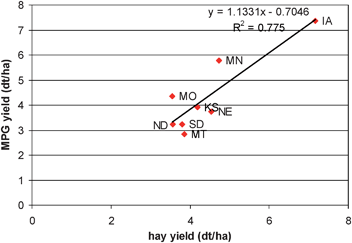Fig. 1 State-average MPG yield vs. hay yield in selected states.

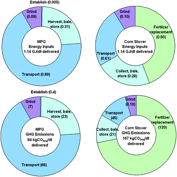
Delivered MPG costs and associated energy use and GHG emissions are estimated (details in the Appendix) assuming that in the establishment year seeds are purchased and the soil is ploughed and planted. The field is then harvested annually (after senescence) for thirty years (the assumed physical life of the conversion facility). Every year, MPG are mowed and raked and then gathered in large rectangular bales containing 95% of the produced biomass. Bales are moved to the field edge, where they are tarped and stored, losing 7% of their dry matter in the process.²² Bales are then hauled by trucks (42 bales, or about 15 dry t, per truck-load) to the plant where they are ground to the appropriate size for the conversion process. Providing 10⁶ t of MPG to a plant with a 3% planting density involves a planting area of about 0.2 million hectares but a biomass collection area larger than 7 million hectares, resulting in an average one-way hauling distance of 141 km. The energy requirements and greenhouse gas emissions associated with MPG production and delivery amount to 1.14 GJ and 84 kgCO_2eq per dry t, respectively, with transportation the dominant component (Fig. 2, Table 2).

Table 2 Estimated energy inputs and GHG emissions associated with production and delivery of MPG and corn stover in Illinois. Calculation details are given in the Appendix

	MPG	Corn stover
Gross yield (dry t/ha/yr)	5.38	9.34
Delivered yield (dry t/ha/yr) ^a	4.75	3.82

---

	MPG		Corn stover
	Energy per delivered tonne (MJ/dt)	GHG emissions per delivered tonne (kg CO2eq/dt)	Energy per delivered tonne (MJ/dt)	GHG emissions per delivered tonne (kg CO2eq/dt)
a Delivered yield is gross yield less collection and storage losses. b Establishment consists of plowing, and seed drilling. MPG are established in the first year. Associated energy requirements and emissions are divided equally over the 30 years of lifetime of the crop. No establishment energy and emissions are charged for corn stover. c Harvest of MPG involves mowing, raking into windrows, field-drying to 20% moisture, and then square-baling. Corn stover harvesting is similar to MPG harvesting, but mowing occurs during harvest of the primary crop and shredding is required before raking. Field-drying reduces moisture content to 15%. d After baling, a Stinger Stacker 4400 collects and piles bales at field edge for manual tarping with the help of a telescopic handler. e Bales are loaded and unloaded with a telescopic handler on a flatbed trailer truck. Transportation includes empty return of trucks. Average one-way transport distances are 141 km for MPG and 44 km for corn stover. f At the conversion facility, bales are fed to the grinder using a telescopic handler.
Establishment
Ploughing	2.3	0.17	—	—
Seeding	1.8	0.13	—	—
Harvest/collection
Mower	78.4	5.77	—	—
Shredder	—	—	35.4	2.60
Wheel rake (V formation)	31.4	2.31	38.9	2.86
Large rectangular baler	80.0	5.89	99.1	7.30
Nutrient replacement	—	—	504.1	89.06
N2O release from nitrogen	—	—	—	31.21
In-field transport & storage
Stinger Stacker	53.6	3.95	57.0	4.19
Tarping	25.6	1.89	27.2	2.00
Transportation
Truck loading	13.6	1.00	14.4	1.06
Truck hauling	750.4	55.27	251.9	18.55
Truck unloading	8.1	0.60	8.6	0.64
Preparation for conversion
Telescopic handler	13.6	1.00	14.4	1.06
Grinder	81.8	6.03	86.9	6.40
TOTAL per dry tonne delivered	1,140.5	84.0	1,137.9	166.95
TOTAL per GJ HHV delivered	60.83	4.48	65.34	9.59

---

Fig. 2 Energy use and GHG emissions for production and delivery of MPG (left side of figure) and stover (right side of figure) in Illinois.

The average cost of delivered MPG is $134/tonne (dry basis), or $7.15/GJ_HHV. (Calculation details are given in the Appendix.) Land rent and truck transportation costs together account for over 60% of this cost (Table 3). The per-hectare land rent was assumed equal to the average 2007 rental rate for CRP land in Illinois. CRP rental rates reflect the opportunity cost of not using these lands for other revenue-generating purposes such as low-productivity agriculture or recreation.

Table 3 Average cost estimated for Illinois of corn stover and MPG delivered to a conversion facility (2007 $ per delivered dry tonne). Calculation details are given in the Appendix

	MPG	Stover
a For MPG, land rent is assumed to be the average CRP contract payment for 2007: $ 255/ha/yr.^30 No land rent is charged to corn stover. b For MPG, establishment costs consist of seeds ($ 247.1/ha for a mix of C4 perennial grasses and forbs plus $ 271.8/ha for a mix of 4 legumes^18), plowing, and drilling. No establishment costs are charged to corn stover.
Land rent	53.69	—
Establishment	8.65	—
Seeds	7.64	—
Ploughing	0.48	—
Seeding	0.53	—
Harvest/collection	21.24	32.91
Mower	8.65	—
Shredder	—	3.57
Wheel rake (V formation)	2.93	3.63
Large rectangular baler	9.66	11.96
Fertilizer replacement	—	13.75
In-field transport & storage	12.89	13.69
Stinger Stacker	9.12	9.69
Tarping	3.77	4.00
Transportation	30.89	12.30
Truck loading	1.66	1.76
Truck hauling	28.24	9.48
Truck unloading	0.99	1.06
Preparation for conversion	6.73	7.15
Telescopic handler	1.66	1.76
Grinder	5.07	5.39
TOTAL COST, 2007$/dry t delivered	134.07	66.06
TOTAL COST, 2007$/GJ HHV delivered	7.15	3.79

---

For corn stover, we assume a gross weight yield per hectare equal to the corn grain yield (dry basis).^23,24 For Illinois, the average corn yield in 2007 was 10.98 tonnes/ha,¹⁹ or 9.34 t/ha on a dry basis. We assume the latter figure to be the gross stover yield (dry basis). Some portion of the stover must be left on the field for soil maintenance. The amount that must be left varies with local soil conditions and climate.^25,26 When removing stover, as much as 50–70% of the gross yield remains on the field due to machinery inefficiencies during collection and baling.²⁷ Our assumed machinery inefficiencies (based on Sokhansanj and Turhollow²⁴) and storage losses together result in 59% of the gross yield of stover being left on the field (see Appendix). We assume that this is a good proxy for the average amount of stover that must be left on the field for soil maintenance.

We note that our estimates of stover removal are generally lower than estimates of acceptable removal by Graham, et al.,²⁸ who took into consideration local soil moisture, water and wind erosion, crop rotation, and irrigation and tillage practices. We also note that some recent research²⁹ suggests that the amount of stover that must be left on the soil to sustain soil organic matter is larger than the amount needed to control wind and water erosion.

Delivered costs, associated energy use, and GHG emissions are estimated (see Appendix) assuming the stover is shredded and raked after the corn harvest, then packed in large rectangular bales that are moved to the field edge where they are tarped for storage. Bales are trucked to a conversion facility, where the biomass is sized for feeding to the process. In order to account for the replacement of nutrients removed with the stover, our cost, energy use, and GHG emissions estimates all take into account nutrient-replacement fertilizer. Transportation distances are estimated assuming that the stover is distributed on land around the plant at the average density of land planted with corn in Illinois—37% in 2007.¹⁹ Delivering 10⁶ t/yr stover involves a collection area of around 700,000 hectares, or an average one-way transport of 44 km.

The estimated energy use and GHG emissions associated with collecting, storing, and delivering corn stover are 1.14 GJ and 167 kgCO_2eq per dry t, respectively, with fertilizer replacement accounting for the largest component (Fig. 2 and Table 2).

With costs of establishment and land rent attributed to the primary product (corn grain), the average delivered cost of stover is $ 66 per dry tonne ($ 3.8/GJ_HHV) (Table 3).

Delivered costs were also estimated for alternative delivery rates for stover (see Table 4); our model predicts that the delivered cost per tonne will change only with the required average transportation distance. For annual delivery rates from 0.5 to 3 million t, the average cost increases from $ 3.6/GJ to $ 4.2/GJ ($ 63/dt to $ 73/dt). As shown in Table 4, these modest cost increases with scale are likely to be more than offset by capital cost scale economy benefits of larger conversion facilities. Thus, the optimum scale of a conversion facility is likely to be limited not by feedstock transport costs but rather by issues like traffic congestion and public perceptions—note that delivering 3 million dt/yr to a facility using trucks with 15 dt capacity would require unloading an average of 23 trucks per hour, 24 hours per day (Table 4).

Table 4 Average cost estimated for delivered corn stover in Illinois as a function of total annual delivery rate. Required number of trucks (15 dt capacity) unloaded per hour at a conversion facility is also shown

Stover delivery rate, 10^6 dry t/yr →	½	1	2	3
Delivered cost, $ per GJHHV	3.6	3.8	4.0	4.2
Delivered cost, $ per dry tonne	63	66	70	73
# of trucks unloaded per hour	4	8	15	23

---

3 Conversion facility design

Fig. 3 is a simplified block diagram of the CBTL plant design considered here. Coal and biomass are gasified in separate gasifiers before the resulting synthesis gas streams are mixed for further processing. Synthesis gas that is not converted into FTL fuels in one pass through the synthesis reactor is used to generate co-product electricity in a gas turbine combined cycle. This “once-through” (OT) process design offers more attractive economics under a wide range of conditions compared to a design that recycles (RC) unconverted gas to increase FTL output.^5,31 (We provide some RC results for comparison.)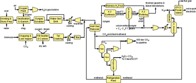

Fig. 3 Assumed process configuration for co-production of FTL fuels and electricity from coal plus biomass with capture and storage of byproduct CO₂. If CO₂ storage were not pursued, the plant design would be essentially identical to the one shown here, except that the two CO₂ compressors in this diagram would not be used and these pure streams of CO₂ would simply be vented.

One important feature of our plant design is the production of both finished diesel and gasoline blendstocks. This is in contrast to most proposed FTL plants, which would produce middle distillates (a mix of jet fuel and heavy diesel) plus naphtha, which would be sold as a feedstock to the chemical process industry. Because our analysis assumes the presence of a widespread CBTL industry, our plant design includes naphtha upgrading to finished gasoline, for which the market is much larger than for naphtha as a chemical feedstock. The latter market would be quickly saturated if a CBTL industry were to be widespread.

Our baseline CBTL plants have an input biomass capacity of 3,044 dry t/day (consuming 1 million t per year), but we also examine plants with smaller and larger biomass input capacities in the corn stover case. In all baseline CBTL-OT-CCS cases [both coal + stover (C + S) and coal + MPG (C + M)], the coal input rate is set such that the FTL fuels are characterized by a zero net fuel-cycle-wide GHG emission rate, considering all of the GHG flows indicated in Fig. 4. We neglect GHG emissions embodied in plant equipment and associated with construction of the conversion facility. For coal-fed facilities that vent CO₂, these emissions are small (e.g., 1% or less in the case of a coal-fired power plant that vents its CO₂³²). For facilities with CCS, these emissions will be larger as a fraction of total emissions, since total emissions are far smaller than with CO₂ venting. Future analysis of CBTL-CCS systems should take into account such emissions.

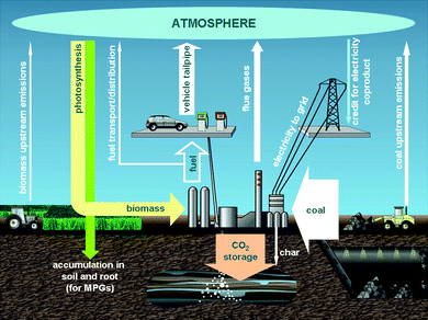Fig. 4 The GHG flows considered in designing a CBTL-CCS system so that the net fuel cycle-wide GHG emission rate for FTL liquids = 0: the biomass:coal input ratio is adjusted until the net flow of GHGs to the atmosphere equals the net flow of GHGs from the atmosphere.

For GHG accounting purposes, we assign to the electricity exported from the site a GHG emissions rate equal to the fuel-cycle emissions rate for a stand-alone coal-IGCC plant with CCS (90% of CO₂ captured), because of the expectation that most new coal power plants to be built in the US will utilize CCS. (Note, however, that the amount of emissions charged to electricity is arbitrary and does not impact overall economics, which depends only on the total system GHG emission rate).

Table 5 shows our simulation results, including several (C + S) cases that differ from the baseline cases. (C + S)′TL-OT-CCS has the same stover input rate as the baseline case but a stover:coal input ratio that gives rise to a GHG emission rate for FTL fuels that is the same as for the crude oil products displaced. Three other stover options have the same stover:coal input ratio as the baseline case but different stover feed rates. (The latter cases are discussed further in the next section.) For comparison, Table 6 shows results developed using the same analytical framework for four CTL and four BTL systems. Two of the CTL systems and all of the BTL systems utilize recycle of syngas (RC) unconverted after a single pass through the synthesis reactor to maximize FTL production. The others, including all of the CBTL designs in Table 5, utilize once-through (OT) synthesis, resulting in a substantial electricity co-product. For the CTL plants, the coal input rate, 24,297 as-received t/day, is fixed at the rate required for the RC designs to produce 50,000 bbl/day of petroleum-equivalent FTL fuels.

Table 5 Performance simulation results for various CBTL systems using “once-through” (OT) synthesis^a

Distinguishing feature →	Baseline cases			Lower S:C ratio	Scaled baseline (-OT-CCS cases)
Process configuration →	(C + M)TL-OT-CCS	(C + S)TL-OT-V	(C + S)TL-OT-CCS	(C + S)′TL-OT-CCS	(C + S)TL- Scale½	(C + S)TL-Scale2	(C + S)TL-Scale3
a Process configuration acronyms: C = coal; M = mixed prairie grasses; S = corn stover; (C + S)′ = coal + corn stover with S:C ratio different from baseline S:C ratio. For (C + S)′TL-OT-CCS, the GHG emission rate for FTL fuels equals that for the crude oil products displaced when S is consumed at a rate of 1 million dry tonnes per year. V refers to venting CO2 and CCS refers to CO2 capture and storage. The configurations called Scale½, Scale2, and Scale3 refer to plants with the same configuration and stover:coal ratio as the baseline (C + S)TL-OT-CCS plants, but consuming ½, 2, and 3 million dry t/year of stover. b Ratio of diesel to gasoline: 61/39 (LHV energy basis), 57/43 (volume basis). Volumetric rates of FTL fuels are reported here as the volumetric rate of crude oil products displaced containing the same amount of energy (LHV basis). c Electricity co-product GHG credit assumed equal to lifecycle emissions from stand-alone coal-IGCC with 90% CO2 capture (138 kgCO2 equivalent/MWh, which includes 1.2 kgCeq per GJLHV coal accounting for coal mining and transportation emissions).
Coal input capacity
As-received, metric t/day	6,689	3,275	3,275	19,650	1,638	6,550	9,825
Coal, MW LHV	2,002	980	980	5,882	490	1,960	2,940
Coal, MW HHV	2,099	1,028	1,028	6,166	514	2,056	3,084
Biomass input, 10 ^6 dry metric t/y (90% cap factor)	1	1	1	1	½	2	3
Biomass input capacity
As-received metric t/day	3,581	3,805	3,805	3,805	1,903	7,610	11,415
Biomass, MW LHV	601	549	549	549	275	1,098	1,647
Biomass, MW HHV	661	614	614	614	307	1,228	1,842
% biomass HHV basis	23.9%	37.4%	37.4%	9.05%.	37.4%	37.4%	37.4%
Total FTL production capacity
Diesel + gasoline, MW LHV	821	484	484	2,040	242	968	1,452
Diesel + gasoline, MW HHV	883	521	521	2,196	261	1,042	1,563
Bbl/day crude oil products displaced	13,039	7,691	7,692	32,413	3,846	15,384	23,076
Electricity
Gross production, MW	609	361	365	1,502	183	730	1,095
On-site consumption, MW	203	75	119	515	60	238	357
Net export to grid, MW	406	286	246	987	123	492	738
Energy Ratios
FTL out (HHV)/Energy in (HHV basis)	32.0%	31.7%	31.7%	32.4%	31.7%	31.7%	31.7%
Net electricity/Energy in (HHV)	14.7%	17.4%	15.0%	14.6%	15.0%	15.0%	15.0%
FTL (HHV) + electricity/Energy in (HHV)	46.7%	49.1%	46.7%	46.9%	46.7%	46.7%	46.7%
FTL Yield (Liters gasoline equiv/dry tonne biomass)	736	434	434	—	434	434	434
C input as feedstock, kgC/second	66	39	39	161	20	78	117
C stored as CO2	50.9%	0	51.7%	51.3%	51.7%	51.7%	51.7%
C in char (unburned)	6.2%	6.9%	6.9%	5.5%	6.9%	6.9%	6.9%
C vented to atmosphere	18.4%	69.2%	17.5%	18.2%	17.5%	17.5%	17.5%
C in FTL	23.9%	23.3%	23.3%	24.3%	23.3%	23.3%	23.3%
C stored, tCO 2 per hour	442	—	272	1,087	136	544	816
C stored, 10 ^6 tCO 2 /yr (90% capacity factor)	3.49	—	2.14	8.58	1.07	4.28	6.42
Net lifecycle GHG emissions for FTL
kgCO2eq/GJ FTL LHV	−5.8	153	1	91.6	1	1	1
Relative to rate for crude oil products displaced	−0.10	1.67	0.01	1.00	0.01	0.01	0.01

---

Table 6 Coal-only and biomass-only performance simulation results developed using framework and assumptions consistent with CBTL results. (See Kreutz et al.⁵ for details of coal-only results.)

Process configuration ^a →	Coal to Liquids				Biomass to Liquids
	CTL RC-V	CTL-RC-CCS	CTL-OT-V	CTL-OT-CCS	MTL-RC-V	MTL-RC-CCS	STL-RC-V	STL-RC-CCS
a C = coal; M = mixed prairie grasses; S = corn stover; RC = recycle synthesis; OT = once-through synthesis; V = vent CO2; CCS = CO2 capture and storage. The biomass-to-liquids facilities consume 1 million metric dry tonnes per year in all cases. b See notes b and c of Table 5. c See notes b and c of Table 5.
Coal input rate
As-received, metric t/day	24,297	24,297	24,295	24,295	—	—	—	—
Coal, MW LHV	7,272	7,272	7,272	7,272	—	—	—	—
Coal, MW HHV	7,625	7,625	7,624	7,624	—	—	—	—
Biomass input rate
As-received metric t/day	—	—	—	—	3,581	3,581	3,805	3,805
Biomass, MW LHV	—	—	—	—	601	601	549	549
Biomass, MW HHV	—	—	—	—	661	661	614	614
% biomass HHV basis	—	—	—	—	100%	100%	100%	100%
Total FTL production capacity
Diesel + gasoline, MW LHV	3,147	3,147	2,307	2,307	278	278	247	247
Diesel + gasoline, MW HHV	3,387	3,387	2,483	2,483	299	299	266	266
Bbl/day crude oil products displaced	50,000	50,000	36,653	36,652	4,414	4,415	3,924	3,925
Electricity
Gross production, MW	874	874	1,672	1,664	66	66	63	63
On-site consumption, MW	447	557	393	589	32	42	30	40
Net export to grid, MW	427	317	1,279	1,075	34	24	33	23
Energy Ratios
FTL out (HHV)/Energy in (HHV basis)	44.4%	44.4%	32.6%	32.6%	45.3%	45.3%	43.3%	43.3%
Net electricity/Energy in (HHV)	5.6%	4.2%	16.8%	14.1%	5.2%	3.7%	5.4%	3.7%
FTL (HHV) + electricity/Energy in (HHV)	50.0%	48.6%	49.3%	46.7%	50.5%	49.0%	48.7%	47.1%
FTL Yield (Liters gasoline equiv/dry tonne biomass)	—	—	—	—	249	249	221	221
C input as feedstock, kgC/second	179	179	179	179	17	17	16	16
C stored as CO2	0	51.5%	0	51.1%	0.0%	51.4%	0.0%	53.6%
C in char (unburned)	5.0%	5.0%	5.0%	5.0%	9.8%	9.8%	9.8%	9.8%
C vented to atmosphere	60.3%	8.9%	69.6%	18.6%	57.2%	5.8%	59.2%	5.6%
C in FTL	33.7%	33.7%	24.7%	24.7%	32.2%	32.2%	30.2%	30.2%
C stored, tCO 2 per hour	—	1,217	—	1,207	—	112	—	111
C stored, 10 ^6 tCO 2 /yr (90% capacity factor)	—	9.60	—	9.52	—	0.88	—	0.87
Net Lifecycle GHG Emissions for FTL
kgCO2eq/GJ FTL LHV	200	94	259	118	−167	−277	−10	−133
Relative to rate for crude oil products displaced	2.18	1.03	2.83	1.28	−1.8	−3.0	−0.1	−1.5

---

In Tables 5 and 6, the process configuration acronyms describe the fate of CO₂, with –V indicating venting and –CCS indicating capture and storage. For all systems involving CO₂ capture, it is assumed that the captured CO₂ is transported 100 km to wells where the CO₂ is injected into a deep saline formation 2 km underground for storage, and the maximum rate of CO₂ injection per well is 2500 tonnes per day.

Several observations follow from Tables 5 and 6:

• Comparing CTL-RC-V and CTL-OT-V options highlights the trade-off between FTL production and electricity exports in RC vs. OT designs: FTL output falls by ¼ from the RC to the OT design, while the net electricity exported is tripled. The additional electricity in the OT case is produced with efficiencies well in excess of those that can be achieved in standalone coal-IGCC systems.^5,31 With biomass co-procesing in an OT configuration (CBTL-OT) similarly high marginal electricity generating efficiencies are achieved.

• Without CCS, the GHG emission rates for coal-only FTL fuels production and use are more than double those for the crude oil products displaced (COPD). The CBTL system in Table 5 without CCS also has a high GHG emission rate for FTL fuels (1.67 × that for the COPD), though not as high as for the coal-only systems. With CCS, coal-only systems have emission rates close to those of the COPD. For the baseline CBTL systems, the net GHG emission rates for FTL fuels are zero (by design, through selection of the ratio of coal-to-biomass input). The GHG emission rates for the BTL systems with CCS are strongly negative, due to storage of photosynthetic CO₂. Emissions are slightly negative for BTL systems without CCS due partly to the incomplete conversion of biomass in the gasifier (see Table 6), with landfilling of the char (residual unconverted carbon), thereby sequestering it from the atmosphere, and partly to the allocation to the coproduct electricity the GHG emission rate for a coal IGCC-CCS power plant with 90% capture.

• Constrained by the biomass feedstock limitation of 10⁶ t/yr and the objective of producing FTL fuels with zero net GHG emissions, the outputs and the amount of coal used for the (C + S)TL-OT-CCS and (C + M)TL-OT-CCS baseline systems are much less than for the CTL systems. However, the outputs of the (C + S)′TL-OT-CCS system having the same rate of biomass input as the (C + S)TL-OT-CCS baseline case but a much smaller stover:coal input ratio are almost as large as for the CTL-OT-CCS systems.

• Coal input for the (C + M)TL-OT-CCS design is higher than for the corresponding (C + S)TL-OT-CCS design because the added carbon storage in soil and roots with MPG offsets the added carbon emission from higher coal use. The higher coal input with the MPG biomass leads to considerably more FTL fuels and power production than when corn stover biomass is used.

• For the (C + S)TL-OT baseline design, net electricity exports fall modestly (14%) when CO₂ is captured rather than vented. The relatively small electricity penalty associated with CCS—compared to IGCC, for example—is a general feature of synfuel production: because a stream of nearly-pure CO₂ is generated as a natural part of the FTL production process, the thermodynamic penalty for CO₂ capture is very low. The largest single energy penalty in adding CCS is for compression of the captured CO₂ to enable pipeline transport and injection underground.⁵

• The effectiveness of CBTL systems in using biomass to make low-carbon liquid fuels is evident in the “FTL yield” (under Energy ratios in Table 5), expressed in liters of gasoline equivalent per dry tonne of biomass input: 434 for the (C + S)TL-OT-CCS system and 736 for the (C + M)TL-OT-CCS system. For comparison, the STL-RC-CCS and MTL-RC-CCS systems yield 221 to 249 liters of gasoline equivalent per dry tonne of input biomass (Table 6), and expected yields for another biofuel, cellulosic ethanol, are in a similar range (213 to 224 liters of gasoline equivalent per dry tonne³³). The high yields for CBTL-OT-CCS systems arise, of course, because the plants use coal in addition to biomass.

4 Economics

We examine overall system economics for a generic Illinois plant site. Three geographic issues are germane to this analysis: proximity of the conversion facility to the biomass resources, proximity to coal mines, and proximity to sites for carbon storage. Fig. 5 gives a representation of these issues: biomass availability (using the methodology described earlier) on a county-by-county basis; the location of active and inactive coal mines (as of the mid-1990s);³⁴ and the thickness of the Mt. Simon sandstone formation, where CO₂ would most likely be stored under Illinois.³⁵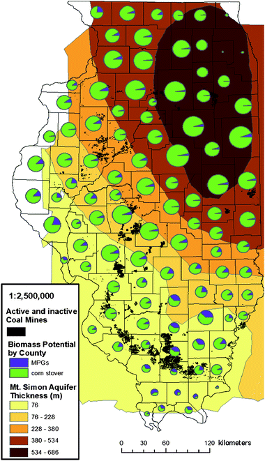

Fig. 5 Illinois' coal, saline aquifer, and potential biomass resources. Total state biomass potential is apportioned by county according to fraction of corn production and CRP acreage in each. Information on the Mt. Simon aquifer is based on maps provided in 2007 by the Midwest Geological Sequestration Consortium.³⁶

Given that the potential availability of MPG and corn stover are relatively high in Illinois (technical potential of ∼2 million and ∼20 million t/yr delivered, respectively) and relatively uniformly dispersed, access to mine mouth coal and to CO₂ injection sites may largely determine plant location.

Possible attractive sites that satisfy both of these requirements can be identified using the data presented in Fig. 5. Coal underlies about 65% of Illinois' land area, and recoverable reserves account for nearly 10% of the U.S. total.

Table 7 shows the total plant cost (TPC) estimated using the framework and sources in Kreutz et al.⁵ for the CBTL plant designs described in Table 5. Table 8 shows costs for the CTL and BTL plants described in Table 6. In both Tables 7 and 8, these are “Nth plant” cost estimates. Significant scale economies are apparent, with the large CTL facilities (Table 8) and the (C + S)′TL-OT-CCS facility having considerably lower specific capital costs ($ per barrel/day of FTL production capacity) than the other CBTL facilities (Table 7). The specific capital costs for BTL plants, despite being smaller in scale, are below those for all but the largest CBTL plants because the specific capital cost index does not reflect the electricity output and because BTL plants are designed for maximum liquids output, while the CBTL plants co-produce substantial electricity.

Table 7 Installed capital costs and levelized FTL production costs with zero GHG emissions price for plants described in Table 5

Distinguishing feature →	Baseline cases			Lower S:C ratio	Scaled baseline (-OT-CCS cases)
Process configuration →	(C + M)TL-OT-CCS	(C + S)TL-OT-V	(C + S)TL-OT-CCS	(C + S)′TL-OT-CCS	(C + S)TLScale½	(C + S)TLScale2	(C + S)TLScale3
Installed capital cost 10 ^6 2007$
Air separation unit, O2 &N2 compression	277	149	161	638	113	297	426
Biomass handling, gasification, & gas cleanup	264	270	254	252	137	444	622
Coal handling, gasification, & quench	472	266	266	1217	143	465	652
All water gas shift, acid gas removal, Claus/SCOT	232	131	149	596	97	230	351
CO2 compression	32	1	23	63	15	37	49
Fischer-Tropsch synthesis & refining	240	164	164	474	99	268	361
Naphtha upgrading to gasoline	47	35	35	80	24	52	66
Power island topping cycle	129	76	79	262	47	144	194
Heat recovery and steam cycle	250	151	150	603	83	276	395
Total plant cost (TPC), 10 ^6 2007$	1,944	1,245	1,281	4,183	756	2,212	3,115
Specific TPC, 2007$ per bbl/day	149,092	161,870	166,577	129,051	196,628	143,769	134,984
Levelized FTL cost, $/GJ LHV
Capital charges	12.9	14.0	14.4	11.1	17.0	12.4	11.6
O&M charges	3.3	3.6	3.7	2.9	4.4	3.2	3.0
Coal (@ $1.44/GJHHV)	3.7	3.1	3.1	4.4	3.1	3.1	3.1
Biomass (see Table 4 for biomass prices)	5.8	4.8	4.8	1.1	4.6	5.1	5.3
CO2 disposal charges	1.0	0.0	1.2	0.7	1.6	.9	0.8
Electricity sales (@$60/MWh)	−8.2	−9.8	−8.5	−8.1	−8.5	−8.5	−8.5
Total, $/GJ LHV	18.4	15.6	18.7	12.2	22.2	16.3	15.4
Total, $/gallon gasoline equiv	2.2	1.9	2.2	1.5	2.7	1.9	1.8
Breakeven oil price (BEOP), $/barrel	88	73	90	54	109	77	72
Avoided GHG cost, $/tCO 2 equivalent	no estimate	—	22	no estimate	no estimate	no estimate	no estimate

---

Table 8 Installed capital costs and levelized FTL production costs with zero GHG emissions price for plants described in Table 6

Process Configuration →	Coal to Liquids				Biomass to Liquids
	CTL-RC-V	CTL-RC-CCS	CTL-OT-V	CTL-OT-CCS	MTL-RC-V	MTL-RC-CCS	STL-RC-V	STL-RC-CCS
Installed Capital Cost 10 ^6 2007$
Air separation unit, O2 &N2 compression	815	815	705	741	95	95	91	91
Biomass handling, gasification, & gas cleanup	0	0	0	0	266	266	255	255
Coal handling, gasification, & quench	1,476	1,476	1,476	1,476	0	0	0	0
All water gas shift, acid gas removal, Claus/SCOT	844	844	638	730	58	58	55	55
CO2 compression	0	67	0	59	1	13	1	13
Fischer-Tropsch synthesis & refining	766	766	523	523	126	127	117	117
Naphtha upgrading to gasoline	103	103	86	86	26	26	24	24
Power island topping cycle	35	35	278	286	0	0	0	0
Heat recovery and steam cycle	840	840	701	695	64	64	60	60
Total plant cost (TPC), 10 ^6 2007$	4,878	4,945	4,407	4,597	636	648	603	615
Specific TPC, 2007$ per bbl/day	97,568	98,908	120,239	125,434	144,084	146,714	153,697	156,623
Levelized FTL cost, $/GJ LHV
Capital charges	8.4	8.5	10.4	10.8	12.4	12.7	13.3	13.5
O&M charges	2.2	2.2	2.7	2.8	3.2	3.3	3.4	3.5
Coal (@ $1.44/GJHHV)	3.5	3.5	4.8	4.8	0.0	0.0	0.0	0.0
Biomass	—	—	—	—	17.0	17.0	9.4	9.4
CO2 disposal charges	0.0	0.5	0.0	0.7	0.00	1.3	0.0	1.5
Electricity sales (@$60/MWh)	−2.3	−1.7	−9.2	−7.8	−2.1	−1.5	−2.2	−1.5
Total, $/GJ LHV	11.8	13.1	8.58	11.3	30.6	32.8	23.9	26.4
Total, $/gallon gasoline equiv	1.4	1.6	1.0	1.4	3.7	3.9	2.9	3.2
Breakeven oil price (BEOP), $/barrel	53	59	35	50	155	167	118	132
Avoided GHG cost, $/tCO 2 equivalent	—	12	—	21	—	21	—	21

---

We estimate levelized FTL production costs for all cases described above. Key assumptions include owner cost (OC) that is 10% of TPC, interest during construction (IDC) that is 7.2% of TPC, a 14.4% capital charge rate on the total plant investment (TPI = TPC + IDC), annual non-fuel operation and maintenance costs equal to 4% of TPC, and a 90% capacity factor.

For a given plant design (e.g., CTL-RC in Table 8), the difference in cost between a design with and without CCS is small—primarily the cost for CO₂ compression, contributing to relatively low avoided GHG emission costs (Table 7 and Table 8, bottom row). [The cost of GHG emissions avoided is the increment in levelized cost ($/GJ) for FTL fuels in shifting from a reference plant that vents CO₂ (–V) to one with CO₂ capture and storage (–CCS), divided by the reduction in the GHG emission rate (t CO_2eq/GJ) in shifting from the –V plant to the –CCS plant. In this formula, the costs do not include a charge for GHG emissions of the systems, but the electricity coproduct credits are valued at a GHG emissions price equal to the cost of avoided emissions. The costs of GHG emissions avoided presented in Tables 7 and 8 are for the case where the reference –V plant has the same basic configuration as the –CCS plant that replaces it.]

The total levelized costs of FTL fuels production for CTL systems (Table 8) are lower than for CBTL systems (Table 7) when zero price is assigned to GHG emissions, and the CTL-OT-V design offers the lowest FTL fuel cost. In contrast, the production costs for BTL plants (at zero GHG emissions price) are much higher than for CBTL systems, due both to the smaller scale of the BTL plants and the higher average feedstock prices paid.

The so-called breakeven oil price (BEOP) – the price of crude oil at which the wholesale price of crude oil products displaced equals the FTL fuels cost (on a $ per GJ_LHV basis) – is an important economic performance index, the calculation of which is described by Kreutz, et al.⁵ CTL systems have BEOPs of $ 35 to $ 59 per barrel with zero price on GHG emissions. BTL systems have BEOPs at the other end of the range estimated in this work, $ 118/bbl to $ 167/bbl. CBTL system BEOPs fall in an intermediate range, from $ 73/bbl to $ 90/bbl at the baseline plant scale. Doubling the scale of the CBTL-OT-CCS plant reduces the BEOP by 14% (“Scale2” plant in Table 7), with a further reduction coming with still larger scale (“Scale3” in Table 7). In these larger CBTL plants, the higher unit price for biomass (Table 4) is more than offset by the reductions in unit capital costs that come with larger conversion facility size. (In practice, conversion efficiencies might also improve with scale. We have assumed fixed efficiencies for this simplified scale analysis, so the BEOP reductions with scale may be underestimated here.)

Despite a higher cost for MPG than for corn stover (Table 3), the FTL production cost is nearly the same for a CBTL-OT-CCS system using MPG [(C + M)TL-OT-CCS] or stover [(C + S)TL-OT-CCS]. This is due primarily to the economies of scale for the larger plant using MPG: for the same biomass input rate as the plant using stover, more coal can be used while still producing zero-GHG-emitting FTL fuels.

The cost of GHG emissions avoided in all cases is less than $22 per tCO_2eq –considerably lower than avoided costs for stand-alone power generation, because energy and capital penalties of adding CCS are relatively small for synfuels production.⁵

The impacts of non-zero GHG emissions prices on production costs and BEOPs are shown in Figs. 6 and 7, respectively.

Fig. 6 FTL production costs with GHG emission price. [Assumed electricity sale price is $ 60/MWh (US average generation revenue in 2007) + GHG charge at 2007 US grid-average GHG emissions rate of 636 kg CO_2eq/MWh)].

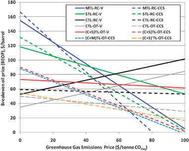Fig. 7 FTL breakeven oil price estimates corresponding to production cost estimates shown in Fig. 6.

Fig. 6 shows that the least costly FTL fuels option is CTL-OT-V until the GHG emissions price reaches $ 21 per tonne, when CTL-OT-CCS becomes the least costly. But at $ 22 per tonne, the least costly option becomes (C + S)′TL-OT-CCS—which provides decarbonized electricity and liquid fuels with the same GHG emissions rate as the crude oil products displaced; it offers less costly FTL fuels than CTL-RC-CCS even at $0 per tonne of CO_2eq. (C + S)′TL-OT-CCS also offers FTL fuels at the least cost of the options considered over a wide range of GHG emissions prices. The (C + S)TL-OT-CCS and the STL-OT-CCS options offer less costly FTL fuels than (C + S)′TL-OT-CCS at GHG emissions prices above $ 70 and $ 85 per tonne, respectively. If MPG-based systems are available as competitors, they [both (C + M)TL-OT-CCS and MTL-RC-CCS] become the least-costly FTL fuels options at GHG emissions above about $ 65 a tonne. STL-RC-CCS does not become the least costly option involving stover until the GHG emissions price exceeds $ 100 a tonne. Notably, CTL-CCS systems are hardly ever the least costly FTL fuels options as long as biomass is available in sufficient quantity at the indicated costs.

Production costs decline with GHG emissions price for several options. Costs decline for BTL-RC options storing biomass-derived carbon as soil/root carbon and/or as CO₂ in geological formations largely because of their strong negative GHG emission rates for FTL fuels. For CBTL-OT-CCS systems that are characterized by zero net GHG emission rates for FTL fuels, costs decline largely because of the growing value of the electricity coproduct with GHG emissions price (see caption for Fig. 6); costs decline at about the same rate for both (C + S)TL-OT-CCS and (C + M)TL-OT-CCS because for these systems the ratio of electricity to FTL fuels output is about the same (0.5). The FTL fuels production cost declines slowly with GHG emissions price even for the STL-RC-V option (involving no soil/root carbon storage) because of the modest negative emission rate assigned to the FTL for this option, as discussed earlier.

Both CBTL-OT-CCS options and the MTL-RC-CCS option become the least costly FTL systems (see Fig. 6) and are competitive with liquid fuels derived from ∼$ 30 a barrel crude oil (see Fig. 7) when the GHG emissions price is ∼$ 65–70 a tonne. The CBTL-OT-CCS options become competitive with CTL-RC-CCS at a much lower GHG emissions price (∼$35/t) but a higher breakeven crude oil price (∼$ 60 a barrel).

In the real world CBTL-OT-CCS options would be characterized by a wide range of biomass:coal input ratios, and the least CBTL-OT-CCS production cost would be realized for a biomass:coal input ratio that increases with the GHG emissions price. Early deployment of CBTL-OT-CCS technologies characterized by low biomass:coal input rates enables biomass to play a significant role in providing liquid fuels at competitive cost long before GHG emissions prices reach levels that enable pure biofuel options to be competitive.

At GHG emission prices in excess of $ 70 a tonne, all the FTL-CCS options involving biomass would be competitive with crude oil priced at $ 40 a barrel (see Fig. 7)—so that at such GHG emission prices investors in these technologies would have a high degree of protection against the risk of oil price collapse. This calculation shows that energy supply security and carbon mitigation need not be conflicting goals for public policy. (For perspective, the International Energy Agency has estimated that GHG emission prices in 2030 should be $ 90 or $ 180 per tonne in OECD + countries, to be consistent with stabilizing atmospheric GHG concentrations at 550 and 450 ppmv, respectively.³⁷)

5 Potential contribution of biomass and coal co-processing in the United States

We applied the same approach as for Illinois to estimate corn stover and MPG availability and cost in other states in the central US using 2007 corn yields and CRP enrolled acreage.

For MPG, we estimated that in 13 states where more than one million tonnes (dry) could be delivered annually, the total delivered MPG potential is about 43 million t/yr from 3.5% of the land area of the states, with an average delivered yield of 4.0 dry t/ha/yr, an average land rent of $ 118/ha/yr, and delivered (1 million dry t/yr) at an average cost of $ 6.1/GJ_LHV ($ 115/dry tonne), Table 9. Delivered costs vary from a low of $ 5/GJ in Colorado due to low land rents and relatively higher density of CRP lands (3.7%) to a high exceeding $ 8/GJ in Missouri due to high land rents. The average transport distance is 140 km for delivering 1 million dry tonnes per year—about the same as for Illinois.

Table 9 State-by-state potential for MPG in the central United States

State	State area [ha]	CRP^30 [%]	CRP payment^30 [2007$/ha/yr]	Hay yield^19 [dry t/ha/yr]	Delivered MPG yield [dry t/ha/yr]	Delivered MPG [dry t/yr]	# of plants (each 10^6 dt/yr)	Average distance [km]	Cost of MPG delivered [2007$/GJ HHV (2007$/dry t)]
Colorado	26,862,614	3.7%	79	5.39	4.78	4,698,122	4.7	127	5 (94.1)
Illinois	14,396,026	3.0%	255	5.37	4.75	2,047,769	2.0	141	7.2 (134.1)
Iowa	14,470,042	5.1%	262	7.16	6.55	4,841,985	4.8	92	5.5 (102.4)
Kansas	21,189,875	6.0%	97	4.19	3.58	4,526,649	4.5	115	6 (112.2)
Minnesota	20,618,837	3.5%	149	4.73	4.11	2,951,066	3.0	140	6.5 (121.3)
Mississippi	12,148,800	3.0%	105	4.19	3.58	1,302,947	1.3	162	6.6 (124)
Missouri	17,841,305	3.3%	165	3.54	2.92	1,728,822	1.7	170	8.6 (161.6)
Montana	37,697,762	3.6%	83	3.85	3.23	4,346,397	4.3	156	6.6 (123.3)
Nebraska	19,909,786	2.5%	141	4.53	3.91	1,976,443	2.0	168	6.8 (128.3)
North Dakota	17,864,615	6.8%	82	3.56	2.94	3,598,682	3.6	118	6.5 (122.2)
Oklahoma	17,784,619	2.2%	81	4.23	3.61	1,439,405	1.4	186	6.5 (121.5)
South Dakota	19,653,956	2.7%	104	3.79	3.17	1,666,455	1.7	182	7.3 (136.5)
Texas	67,804,882	2.4%	87	5.47	4.85	7,741,734	7.7	157	5.4 (101.1)
Total	308,243,120	3.5%	—	—	—	42,866,476	43	—	—
Weighted average	—	—	118	—	4.01	—	—	140	6.1 (115.1)

---

For corn stover, we estimated the potential for 16 states, which together accounted for 95% of US corn production in 2007. Each state examined has the potential to deliver at least one million t/yr (dry) of stover. The total estimated potential for delivered corn stover in these states is about 113 million t/yr from 33.5 million ha (10.8% of the total area) producing an average of 3.4 dry t/ha/yr of delivered stover, Table 10. The average transport distance is 76 km for delivering 1 million dry tonnes per year and the average delivered cost is $ 4.3/GJ_LHV ($ 76/dry tonne).

Table 10 State-by-state potential for corn stover in the central United States

State	State area [ha]	Corn land^19 [%]	Corn yield^19 [wet t/ha]	Delivered stover yield [dry t/ha/yr]	Delivered stover [dry t/yr]	# of plants (each 10^6 dt/yr)	Average distance [km]	Cost of corn stover delivered [2007$/GJ HHV (2007$/dry t)]
Colorado	26,862,614	1.8%	8.91	3.12	1,513,032	1.5	224	6.2 (108.7)
Illinois	14,396,026	37.1%	10.98	3.82	20,511,172	20.5	44	3.8 (66.1)
Indiana	9,289,449	28.3%	9.73	3.40	8,945,890	8.9	54	4.1 (70.6)
Iowa	14,470,042	39.7%	10.73	3.75	21,560,705	21.6	43	3.8 (66.3)
Kansas	21,189,875	7.4%	8.79	3.07	4,848,095	4.8	111	4.9 (85)
Kentucky	10,289,512	5.7%	8.10	2.83	1,660,872	1.7	132	5.3 (91.6)
Michigan	14,712,065	7.3%	7.78	2.72	2,917,736	2.9	119	5.2 (89.9)
Minnesota	20,618,837	16.5%	9.16	3.20	10,889,568	10.9	73	4.4 (76)
Mississippi	12,148,800	3.2%	9.41	3.29	1,278,619	1.3	164	5.4 (94.6)
Missouri	17,841,305	7.8%	8.91	3.12	4,349,967	4.3	107	4.8 (83.9)
Nebraska	19,909,786	19.1%	10.04	3.51	13,354,460	13.4	65	4.1 (72.2)
North Dakota	17,864,615	5.8%	7.28	2.55	2,626,496	2.6	138	5.5 (95.8)
Ohio	10,605,541	14.7%	9.41	3.29	5,127,793	5.1	76	4.4 (76)
South Dakota	19,653,956	10.3%	7.59	2.65	5,371,974	5.4	101	5 (86.8)
Texas	67,804,882	1.3%	9.29	3.25	2,825,392	2.8	260	6.6 (115.5)
Wisconsin	14,066,197	11.7%	8.47	2.96	4,854,755	4.9	90	4.7 (81.5)
TOTAL	311,723,504	10.8%	—	—	112,636,524	113	—	—
Weighted average	—	—	9.60	3.36	—	—	76	4.3 (75.6)

---

The potential MPG and corn stover resources in the states shown in Tables 9 and 10, if used in the baseline CBTL-CCS systems described above, could displace 1.3 million barrels per day of crude oil products (equivalent to ∼10% of US oil imports in 2007) while providing 350 TWh of decarbonized electricity (∼18% of all US coal-fired power generation in 2007).

The biomass potential for coprocessing at CBTL plants is likely to be greater than these calculations suggest. For example, the total land area considered in Table 9 for growing MPG is about 11 million hectares, while the states shown in that table contain a USDA-estimated 64 million hectares (∼1/3 of US total) of abandoned or degraded agricultural land that might be considered for growing MPG.²¹ Other prospectively important biomass supplies include crop residues in addition to corn stover and woody biomass supplies such as urban wood wastes and forest-derived residues (mill residues, logging residues, diseased tree kills, fuel treatment thinnings, and productivity enhancement thinnings).³⁸

6 Conclusions

Plentiful biomass and coal resources in Illinois and good access to CO₂ storage sites make it a good candidate for siting of facilities to co-produce low GHG emission liquid fuels and decarbonized electricity. Under a strong carbon mitigation policy, the economics of such CBTL-OT-CCS facilities appear attractive. The biomass resources in a wider region in the central US could support the production of a nationally-significant amount of zero-GHG transportation fuel and decarbonized co-product electricity. Our analysis shows that energy supply security and carbon mitigation need not be conflicting goals for public policy.

Appendix

Detailed calculation of costs, energy use, and greenhouse gas emissions associated with production, storage, transport, and pre-processing of MPG and corn stover are provided here.

Costs

Delivered biomass costs are estimated using an engineering-economic approach. The costs of field operations are assessed from machinery design parameters, in-field efficiency, and financial assumptions. The cost of transportation from field to conversion facility is estimated assuming that biomass is collected from a circular area around the plant, with a road tortuosity of 1.4 (to take into account the actual transport distance relative to the straightline distance between two points) and planting densities discussed in the main text.

Machinery performances and costs are estimated on the basis of the machinery's rated capacity to work on the field. This approach is widely used to estimate costs of food crop production,^39,40as well as biomass energy feedstock production.^41,42 The equipment's capacity to work on the field is determined from its “effective field capacity” (EFC). EFC is defined as the rate at which a machine performs its primary function (e.g., hectares per hour mowed or tonnes of biomass per hour baled). EFCs are estimated on the basis of machinery characteristics described in the literature.^41–43 For example, in the case of the mower used to cut MPG, the EFC is the product of the theoretical field capacity (width of mower times average speed of travel during cutting) and the mower's “field efficiency”, an empirically-determined ratio of actual-to-theoretical field capacity (Table 11).

Table 11 Horse power, field efficiency, effective field capacity (EFC), and hourly cost of equipment^a

	Power (hp)	Field Eff (%)	EFC	Cost (2007$/hr)
a Notes: Horsepower ratings are from refs. 40,41 and 43. Field efficiencies are from ASAE^44 and Turhollow and Sokhansanj.^43 Tarping of bales, truck loading/unloading, and feeding to grinder are all done using a telescopic handler (JCB 520).
Establishment (for MPG)
Ploughing	160	85	3.44 ha/h	99.6
Seeding	120	70	2.75 ha/h	91.3
Harvest/collection
Mower	120	85	2.10 ha/h	66.5
Shredder	80	80	3.84 ha/h	52.7
Wheel rake	80	85	3.50 ha/h	37.3
Baler (large, rectangular)	160	80	2.75 ha/h	96.9
In-field transport & storage
Stinger stacker	106	85	32 bales/h	137
Tarping	76	90	54 bales/h	46
Transportation
Truck loading	76	85	102 bales/h	46.4
Truck hauling	400	85	1364 bale-km/h	75.7
Truck unloading	76	85	170 bales/h	46.4
Preparation for gasification
Feeding to grinder	76	85	31 bales/h	46.4
Grinder	280	85	26.3 t/h	86.6

---

The EFC is used with an hourly cost of operation to determine the total cost of each operation. The hourly cost for each piece of machinery is estimated (Table 11) as described in the literature^41–43 using the following general assumptions: real discount rate of 7%; 1.1 hours of operating time per hour of field time (to account for travel to/from the field and other similar factors); wage rate of $ 10.28/hr (2007 average in the US for farm labor⁴⁴); machinery purchase price is 90% of list price, and prices are expressed in 2007$ using USDA agricultural price indices;⁴⁵ 1.2 hours of labor per hour of field time; property tax, insurance, and shelter costs are assumed to be 2% of equipment purchase price plus salvage value; lubrication costs are assumed to be 15% of fuel costs; interest is charged on operating expenses (e.g., fertilizers, fuel) and on farm operations (e.g., equipment maintenance and repairs). Fuel use is factored into the hourly cost assuming a fuel price of $ 1.06/liter (diesel fuel) and fuel use estimated as described further below.

Dry matter losses are also factored into the calculation. For MPG, field losses are assumed to be 5% of gross yield and storage losses are assumed to be 7%.²² For corn stover,²⁴ losses are 30% during shredding, 5% during raking, 30% during baling, and 5% during stacking of bales. Storage losses are assumed to be the same as for MPG, 7%.

We illustrate the cost calculation for three operations. First, consider the mower, which contributes the following cost per tonne of delivered biomass:

C_mower = C_h·EFC_area⁻¹·Y⁻¹·(1 − DML_h) ⁻¹·(1 − DML_s) ⁻¹ (1)

where: C_h is the hourly cost ($/h); EFC_area is the effective field capacity (ha/h); Y is the gross yield (dry t/ha); DML_h harvest dry matter loss (decimal fraction, mass basis); DML_s storage dry matter loss (decimal fraction, mass basis). Other equipment for which EFC is expressed on an area basis would involve a similar calculation. Second, consider the stinger stacker, for which EFC is expressed on a per-bale basis. For this (and similarly for other equipment with EFC on a per-bale or per-tonne basis), the cost per tonne of delivered biomass is:

C_stinger = C_h·EFC_weight⁻¹·W_b⁻¹·(1 − DML_s)⁻¹ (2)

where: EFC_weight is the effective field capacity (bale/h) and W_b is the weight of one bale before storage losses (0.45 dry t/bale). The bales are rectangular (1.2 m × 1.2 m × 2.4 m).

Finally, the cost estimate for truck hauling is approached in a similar manner as the other equipment, but since its EFC is expressed in terms of bale-km/h, the trucking cost per t is:

C_truck = C_h·d·EFC_truck⁻¹·W_b⁻¹·(1 − DML_s)⁻¹ (3)

where EFC_truck is the effective field capacity (bale·km/h) that accounts for two-way travel and d is the one-way distance travelled by the truck (km). Each 16-meter flatbed trailer truck carries 42 bales.

Fuel use

Fuel consumption for each operation is estimated in a manner similar to that for costs, but with fuel use per hour substituting for cost per hour. According to Turhollow and Sokhansanj,⁴³ the American Society of Agricultural Engineers (ASAE) recommends that the actual power used by specific models of tractors pulling implements be used to calculate fuel use. In the absence of these data, the ASAE suggests estimating hourly diesel fuel consumption as 0.166 litres/hour of diesel (0.0438 gallons/h) per horsepower of equipment capacity.⁴⁶ We have used this approach, assuming the horsepower of farm implements (or the tractors used to pull the implements) are as listed in Table 11. The MJ of fuel required per hour (F_h) is thus:

F_h = t_field·HP·DR_diesel·E_diesel (4)

where t_field is the number of operating hours per hour of field time (assumed to be 1.1); HP is the horse power of the machinery; DR_diesel is the ASAE-recommended diesel rate (liters per hour per hp); and E_diesel is the lower heating value energy content of diesel fuel (assumed to be 35.8 MJ/liter⁴³).

Greenhouse gas emissions for consumed fuels

Greenhouse gases emissions (CO₂, CH₄, N₂O) are estimated from equipment fuel consumption using emission factors from the GREET model:⁴⁷ 0.597 gCH₄/GJ of fuel used; 0.872 gN₂O/GJ; and 73.384 gCO₂/GJ. The CO₂ equivalent emissions are estimated using the following 100-year global warming potentials of each gas: 1 kgCO_2,eq/kgCO₂; 25 kgCO_2,eq/kgCH₄; 298 kgCO_2,eq/kgN₂O.⁴⁸

Cost, energy, and GHGs for fertilizer

Cost, energy and GHG emissions associated with replacing the nutrient value of corn stover removals with artificial fertilizer are included in the analysis. The replacement fertilizer needed is 1.6 kg_P2O5, 12.2 kg_K2O and 8.1 kg_NH3 per dry t stover removed,²³ with costs assumed to be $ 622/t_P2O5, $ 697/t_K2O and $ 523/t_NH3.⁴⁹ We assume the added fertilizer is applied together with the normal fertilizer used for corn grain production, thereby incurring little added cost for the application.

We neglect the added application cost. The energy cost for the fertilizer is assumed to be the energy required to produce phosphorus, potassium and nitrogen, respectively about 9, 6 and 51 MJ per kilogram of pure element.⁵⁰ GHG emissions are estimated assuming that all of this energy is electricity, with associated GHG emissions of 636 kg CO_2eq/MWh, the 2007 average emissions for the U.S. grid.^5,47 Also, nitrous oxide emissions released from the nitrogen fertilizer to replace nitrogen lost by stover removal are estimated, assuming that 1% of nitrogen contained in the fertilizer is converted in N₂O.⁵¹

Acknowledgements

For financial support, we thank Princeton University's Carbon Mitigation Initiative and its sponsors (BP and Ford); NetJets Inc; The William and Flora Hewlett Foundation; the Italian Ministero dell'Istruzione, dell'Università e della Ricerca (Interlink project II04CE49G8); and LEAP (Laboratorio Energia Ambiente Piacenza). Also, this paper was derived in part from work funded by the National Academy of Sciences, with support from the National Academy of Engineering, National Research Council, the US Department of Energy, General Motors, Intel Corporation, Kavli Foundation, and the Keck Foundation. The contents of this paper are not necessarily accepted or adopted by any of the foregoing organizations.

References

1. M. W. Rosegrant, Biofuels and Grain Prices: Impacts and Policy Responses, Testimony before US Senate Committee on Homeland Security and Government Affairs, Washington, DC, 7 May 2008.
2. J. Fargione, J. Hill, D. Tilman, S. Polasky and P. Hawthorne, Science, 2008, 319, 1235–1238.
3. T. Searchinger, R. Heimlich, R. A. Houghton, F. Dong, A. Elobeid, J. Fabiosa, S. Tokgoz, D. Hayes and T. Yu, Science, 2008, 319, 1238–1240.
4. D. Tilman, R. Socolow, J. A. Foley, J. Hill, E. Larson, L. Lynd, S. Pacala, J. Reilly, T. Searchinger, C. Sommerville and R. Williams, Science, 2009, 325, 270–271.
5. T. G. Kreutz, E. D. Larson, G. Liu and R. H. Williams, Proceedings of the 25th Annual Pittsburgh Coal Conference, Pittsburgh, 2008.
6. R. H. Williams, E. D. Larson and H. Jin, 8th International Conference on Greenhouse Gas Control Technologies, Trondheim, 2006.
7. D. Gray, C. White, G. Tomlinson, M. Ackiewicz, E. Schmetz and J. Winslow, Increasing Security and Reducing Carbon Emissions of the U.S. Transportation Sector: A Transformational Role for Coal with Biomass, National Energy Technology Laboratory, 2007.
8. Western Governors' Association, Transportation Fuels for the Future: A Roadmap for the West, 2008.
9. J. Baardson, S. Dopuch, R. Wood, A. Gribik and R. Boardman, 24th Annual Pittsburgh Coal Conference, Johannesburg, 2007.
10. T. J. Tarka, Affordable, Low-Carbon Diesel Fuel from Domestic Coal and Biomass, DOE/NETL-2009/1349, National Energy Technology Laboratory, 2009.
11. J. Bartis, F. Camm and D. S. Ortiz, Producing Liquid Fuels from Coal: Prospects and Policy Issues, Project Air Force and Infrastructure, Safety, and Environment, United States Air Force and the National Energy Technology Laboratory of the United States Department of Energy, 2009.
12. Energy Information Administration, Annual Energy Outlook 2008, DOE/EIA-0383, 2008.
13. Energy Information Administration, Annual Coal Report 2007, DOE/EIA 0584, 2007.
14. D. Tilman, J. Hill and C. Lehman, Science, 2006, 314, 1598–1600.
15. National Energy Technology Laboratory, Cost and Performance Baseline for Fossil Energy Plants: Volume 1: Bituminous Coal and Natural Gas to Electricity, DOE/NETL-2007/1281 Rev. 1, 2007.
16. T. J. Tarka (National Energy Technology Laboratory, Pittsburgh, PA), personal communication.
17. C. Lehman (University of Minnesota, St. Paul, MN), personal communication.
18. D. Tilman (University of Minnesota, St. Paul, MN), personal communication.
19. USDA/NASS, National Agricultural Statistics Service, 2008.
20. National Agricultural Statistics Service, 2002 US Agricultural Census, App. A: Data Collection and Capture, USDA, 2004.
21. Agricultural Statistics Service, 2002 Census of Agric., USDA, 2004.
22. M. Duffy, On-Farm Costs of Switchgrass Production in Chariton Valley, Iowa State Extension, 2003.
23. P. W. Gallagher, M. Dikeman, J. Fritz, E. Wailes, W. Gauthier, and H. Shapouri, Biomass from Crop Residues: Cost and Supply Estimates, Agricultural Economics Report No. 819, USDA, 2003.
24. S. Sokhansanj and A. R. Turhollow, Appl. Eng. Agr., 2002, 18, 525–530.
25. W. W. Wilhelm, J. M. F. Johnson, J. L. Hatfield, W. B. Voorhees and D. R. Linden, Agron. J., 2004, 96, 1–17.
26. S. Andrews, White Paper: Crop Residue Removal for Biomass Energy Production: Effects on Soils and Recommendations, USDA, 2006.
27. J. E. Atchison and J. R. Hettenhaus, Innovative Methods for Corn Stover Collecting, Handling, Storing and Transporting, National Renewable Energy Lab, Golden, CO, 2004.
28. R. L. Graham, R. Nelson, J. Sheehan, R. D. Perlack and L. L. Wright, Adv. Agron., 2007, 92, 1–11.
29. W. W. Wilhelm, J. M. E. Johnson, D. L. Karlen and D. T. Lightle, Agron. J., 2007, 99, 1665–1667.
30. Farm Service Agency, Conservation Reserve Program: Summary and Enrollment Statistics, USDA, 2007.
31. R. H. Williams, E. D. Larson, G. Liu and T. G. Kreutz, 9th International Conference on Greenhouse Gas Control Technologies, Washington DC, 2008.
32. P. L. Spath, M. K. Mann and D. R. Kerr, Life Cycle Assessment of Coal-Fired Power Production, NREL/TP-570-25119, National Renewable Energy Laboratory, Golden, CO, 1999.
33. America's Energy Future Study Panel on Alternative Transportation Fuels, Liquid Transportation Fuels from Coal and Biomass Technological Status, Costs, and Environmental Impacts, U.S. National Academy of Sciences, 2009.
34. B. J. Stiff, Areas Mined for Coal in Illinois, ISGS GIS Database, Illinois State Geologic Survey, 1997.
35. Midwest Geological Sequestration Consortium, An Assessment of Geological Carbon Sequestration Options in the Illinois Basin, U.S. DOE Contract DE-FC26–03NT41994, 2005.
36. C. Korose (Midwest Geological Sequestration Consortium), personal communication.
37. International Energy Agency, World Energy Assessment 2008, Paris, 2008.
38. R. D. Perlack, L. L. Wright, A. Turhollow, R. L. Graham, B. Stokes and D. C. Erbach, Biomass As Feedstock For A Bioenergy And Bioproducts Industry: The Technical Feasibility Of A Billion-Ton Annual Supply, ORNL/TM-2005/66, Oak Ridge National Laboratory, Oak Ridge, TN, 2005.
39. W. Edwards, Machinery Management, Estimating Farm Machinery Costs, Iowa State Extension, 2005.
40. M. Hanna, Estimating Field Capacity of Farm Machines – Machinery Management, Iowa State Extension, 2001.
41. A. Kumar and S. Sokhansanj, Bioresour. Technol., 2007, 98, 1033–1044.
42. D. Grant, J. R. Hess, K. Kenney, P. Laney, D. Muth, P. Pryfogle, C. Radtke and C. Wright, Feasibility of a Producer Owned Ground-Straw Feedstock Supply System for Bioethanol and Other Products, Idaho National Laboratory, 2006.
43. A. Turhollow, and S. Sokhansanj, Cost methodology for biomass crops, Oak Ridge National Laboratory, 2002.
44. National Agricultural Statistics Service, Farm Labor: Wage Rate by Quarter, USDA, 2008.
45. USDA/NASS, Agricultural prices, 01.31.2008_revision. Agricultural statistics board, 2008.
46. American Society of Agricultural Engineers, Agricultural Machinery Management Data, ASAE D497.4 MAR99, 2003.
47. Argonne National Laboratory, GREET 1.8b The Greenhouse Gases, Regulated Emissions, and Energy Use in Transportation (GREET) Model (release September 2008), 2007.
48. S. Solomon, D. Qin, M. Manning, R. B. Alley, T. Berntsen, N. L. Bindoff, Z. Chen, A. Chidthaisong, J. M. Gregory, G. C. Hegerl, M. Heimann, B. Hewitson, B. J. Hoskins, F. Joos, J. Jouzel, V. Kattsov, U. Lohmann, T. Matsuno, M. Molina, N. Nicholls, J. Overpeck, G. Raga, V. Ramaswamy, J. Ren, M. Rusticucci, R. Somerville, T. F. Stocker, P. Whetton, W.R.A. and D. Wratt, in Climate Change 2007: The Physical Science Basis, eds. S. Solomon, D. Qin, M. Manning, Z. Chen, M. Marquis, K. B. Averyt, M. Tignor and H. L. Miller, Cambridge University Press, Cambridge and New York, 2007.
49. Economic Research Service/National Agricultural Statistics Service, U.S. Fertilizer Use and Price, Average U.S. Farm Prices of Selected Fertilizers, U.S. Department of Agriculture, 2008.
50. J. Hill, E. Nelson, D. Tilman, S. Polasky and D. Tiffany, Proc. Natl. Acad. Sci. U. S. A., 2006, 103, 11206–11210.
51. C. De Klein, R. S. A. Novoa, S. Ogle, K. A. Smith, P. Rochette, T. C. Wirth, B. G. McConkey, A. Mosier and K. Rypdal, in 2006 IPCC Guidelines for National Greenhouse Gas Inventories, ed. H. S. Eggleston, L. Buendia, K. Miwa, T. Ngara and K. Tanabe, IGES, Hayama, Japan.

---