A novel automatic method for the measurement of mercury vapour in ambient air, and comparison of uncertainty with established semi-automatic and manual methods

Abstract

The measurement of mercury vapour in ambient air is required in order to ensure the quality life of the general public. New legislation introduced recently by the European Commission has mandated that sampling and analysis be performed in situ at monitoring sites, and that mass concentration of mercury vapour in ambient air is determined within a maximum uncertainty. This paper presents a novel and innovative automatic method for such in situ measurements of mercury vapour in ambient air using atomic fluorescence spectrometry, where calibration, sampling and analysis are all performed fully automatically without manual intervention. A robust measurement equation and uncertainty budget for this automatic method is developed, and the overall relative expanded uncertainty for an exemplar measurement has been found to be 21%, well below the target expanded uncertainty of 50% set by the European Commission for these measurements. The uncertainty of a semi-automatic method (automatic sampling and analysis, but manual calibration) has also been assessed, and compared with the uncertainty of the novel automatic method, and the uncertainty of a manual (remote sampling and manual calibration and analysis) method presented in a previous study.

---

Introduction

The measurement of ambient air quality is an essential requirement of modern society due to its role in ensuring the health and improving the quality of life of the general public. These measurements also enable compliance with European target values for pollutants in ambient air and pollutants emitted from stationary sources to be assessed, as well as informing government policy development and assessing the effectiveness of abatement strategies.

Mercury is a particularly toxic and persistent pollutant, and its potential for bioaccumulation means that it is particularly insidious, even when exposure is through low-level environmental sources.¹ It is therefore essential to monitor and manage the exposure of the general public to mercury. Mercury vapour‡ is emitted from a large variety of sources—coal-burning power plants are currently the largest anthropogenic source of emissions in the UK, with crematoria and inappropriate disposal of mercury-containing waste also being major contributors.

Measurement of the concentration of mercury vapour in ambient air is a legislative requirement in order to satisfy regional and national legislation such as the European Commission's Fourth Air Quality Daughter Directive.² Emissions from stationary sources are covered by other legislation, such as the US Environmental Protection Agency's Clean Air Mercury Rule;³ documentary standards for these measurements also exist.⁴ In the UK, measuring the concentration of mercury vapour in ambient air at an extensive number of sites across the country ensures the Government's compliance with the Fourth Air Quality Daughter Directive. The National Physical Laboratory undertakes these measurements for the Department for Environment, Food and Rural Affairs (Defra) as part of its UK Heavy Metals Monitoring Network.⁵

Measurements of mercury vapour for the UK Heavy Metals Monitoring Network are currently carried out by sampling ambient air for a period of one to four weeks onto an adsorption tube (containing gold-coated silica as the sorbent material) at the monitoring site. The adsorption tube is then sent to the laboratory for analysis by atomic fluorescence spectrometry. This is hereafter referred to as the ‘manual’ sampling and analysis approach.§

Fig. 1 emphasises the importance of accurate determination of the concentration of vapour-phase mercury as the primary indicator of mercury exposure in ambient air by showing the concentrations of vapour-phase and particulate-phase mercury recorded by the UK Heavy Metals Monitoring Network in 2008.¶ From the figure, where each point represents the average concentrations recorded over a one month period from each of the 13 sites, it can be seen that, with only one exception, the concentration of vapour-phase mercury is between two and four orders of magnitude greater than that in the particulate-phase. The vast majority of this vapour phase mercury is gaseous elemental mercury.⁶

Fig. 1 Plot of the concentrations of vapour-phase mercury and particulate-phase mercury recorded by the UK Heavy Metals Monitoring Network in 2008. Each point represents the average concentration recorded over a one month period from one of the 13 monitoring sites where vapour and particulate-phase mercury are both measured. The dashed diagonal lines indicate where the ratio of vapour phase concentration (y) to particulate phase concentration (x) is 1000, 100 and 10.

The European Commission has introduced legislation via the Fourth Air Quality Daughter Directive² mandating the future use of an alternative method for the measurement of mercury vapour, where sampling and analysis are performed in situ at each monitoring site. This approach, which we hereafter refer to as the ‘programmed’ sampling and analysis approach, has the advantage of being able to provide data over shorter time periods, thus enabling any ‘spikes’ in concentration caused by release episodes to be identified. (Such incidents may easily be lost when using the manual method and sampling for a period of a week or more.) Use of the programmed sampling and analysis approach also improves the cost-effectiveness of a measurement campaign once capital equipment has been purchased, by decreasing operating costs. Working Group 25 of the European Committee for Standardization's (CEN) Technical Committee on Air Quality (CEN TC 264/WG 25) has been tasked with developing a documentary standard method in support of this approach, a final draft of which⁷ is undergoing formal approval prior to publication.

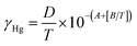
For measurements carried out using the manual sampling and analysis approach, the analyser is typically calibrated using known volumes of mercury-saturated air from a ‘bell-jar’ device. This calibration approach is hereafter referred to as ‘bell-jar calibration’. The bell-jar, which is shown schematically in ESI Fig. A† and described in detail in previous work,^8,9 is a glass vessel containing a small amount of elemental mercury which generates mercury-saturated air within the vessel, which is in equilibrium with the atmosphere via a capillary tube. The temperature of the vapour within the bell-jar is measured with a platinum-resistance thermometer and samples of vapour are taken with a gas-tight syringe through a septum in the top of the bell-jar. Knowledge of the temperature of the mercury-saturated air allows the mass of mercury to be calculated using the empirical relationship (the ‘Dumarey equation’)^10,11 shown in eqn (1):

In this equation, γ_Hg is the saturated mass concentration of mercury vapour in air; T is the temperature of saturated vapour inside the bell-jar; A, B and D are constants equal to −8.1344, 3240.9 K and 3 216 522 K ng ml⁻¹ respectively, and δ is the deviation of the theoretical saturated vapour mass concentration of mercury in the bell-jar from reality (as discussed in detail in ref. 9). For the purpose of this study, where all the measurements that are being compared utilise the Dumarey equation, we have assumed the value of δ to be unity with zero uncertainty. Although a major experimental study has found δ to lie within the range 0.98 ≤ δ ≤ 1.02 by use of an isotope dilution-inductively coupled plasma-mass spectrometry (ID-ICP-MS) technique,¹² the assumption that δ has zero uncertainty is used here as it more clearly allows the reader to identify how the other contributory factors affect the overall uncertainty.

This paper also introduces a novel alternative calibration approach, ‘dynamic calibration’, where calibration takes place with no manual intervention by using a dynamic mercury vapour generator (DMVG) to produce air containing a known mass concentration of mercury, which is then sampled for a known period of time. Dynamic calibration is most suitable for use with the programmed sampling and analysis approach, as this would allow an entire experimental protocol (e.g. a field trial) to be undertaken with no need for manual intervention—this would be particularly useful at remote monitoring sites. Dynamic calibration could of course be used with the manual sampling and analysis approach by performing calibration with adsorption tubes spiked with known masses of mercury, although this would almost certainly not represent an operational improvement.

The different possible combinations of the two sampling and analysis approaches with the two calibration approaches are shown schematically in Fig. 2. In this paper, we focus on the use of the programmed sampling and analysis approach with dynamic calibration (we refer to this combination as the ‘automatic method’). To the best of the authors' knowledge, this is the first time that such a set-up has been used for monitoring of mercury vapour in ambient air with a dynamic calibration in the ng m⁻³ mass concentration range, and so the work presented here is novel and innovative. We also discuss the programmed sampling and analysis approach with bell-jar calibration (we refer to this combination and the ‘semi-automatic method’).

Fig. 2 The mercury vapour measurement methods formed from combination of different sampling and analysis approaches with different calibration approaches. The automatic method is the novel methodology outlined in this paper, and the semi-automatic method is the basis of the draft standard method being prepared by CEN.⁷ The manual method is discussed in detail in ref. 9 and the manual method (spiked tube calibration) is not considered in this paper.

The development of sampling and analysis approaches to measure mercury vapour in ambient air has been an important area of research for many years. Recent developments include a simultaneous method of sampling onto a needle trap and analysis by gas chromatography-mass spectrometry¹³ and a dual amalgamation cold-vapour atomic absorption spectrometry analysis technique.¹⁴ The methods presented in this paper have the major benefit of combining automation with accurate calibration and analysis.

A rigorous assessment of the overall uncertainty of the automatic and semi-automatic methods for the measurement of mercury vapour in ambient air is presented, and the overall uncertainties are then compared with the uncertainty of the ‘manual method’ (the manual sampling and analysis approach with bell-jar calibration, i.e. the method currently used in the UK to provide data for legislative purposes). As discussed in the above paragraph, the fourth possible combination—manual sampling and analysis approach with dynamic calibration—referred to in Fig. 2 as ‘manual method (spiked tube calibration)’ is not discussed.

Experimental

Atomic fluorescence spectrometry

All the methods studied used a ‘Sir Galahad II’ atomic fluorescence instrument (model 10.525, PS Analytical, Orpington, UK) with a permanent trap of a quartz glass adsorption tube containing approximately 30 mg of Amasil (gold-coated silica) material. This gold-coated silica material caused the vapour-phase mercury to form an amalgam on the trap, which was then heated to desorb the mercury into a carrier stream of argon and onto the detector, where the response was recorded.

Before any experiments were undertaken, the linearity of the detector was first checked by injecting a range of known volumes of saturated mercury vapour. For all the experiments reported in this paper, peak height (rather than peak area) was used as this was found to be more reproducible for these trace level measurements, some of which are close to the limit of detection of the atomic fluorescence instrument.

Bell-jar calibration

For bell-jar calibration, a known volume of mercury-saturated air from a bell-jar (PS Analytical; see ESI Fig. A†) was taken using a gas-tight syringe (Vici, Baton Rouge, US) that had been pre-calibrated by measuring the mass of water held by the syringe up to a range of its graduation marks at a given temperature. The temperature inside the bell-jar was measured using a calibrated platinum resistance thermometer (model 2024T, Digitron UK). As discussed previously, detailed studies of the bell-jar calibration method have found the most accurate calibration approach to be the use of a single-point calibration injection of a mass of mercury similar to that expected in the unknown immediately before the analysis of the sample.

Dynamic calibration

For dynamic calibration, a stream of air containing mercury vapour at a known concentration was generated by a dynamic mercury vapour generator (DMVG) (Cavkit model 10.534, PS Analytical) and then further diluted using a dilution stream selector system (model 50.119, PS Analytical), as shown schematically in Fig. 3. The DMVG settings used varied, but the data discussed in this paper were obtained by setting the DMVG to produce an undiluted output with a mercury mass concentration of 5.27 ng l⁻¹. The stream selection system was set to give a nominal dilution factor of 200 : 1 by use of a critical orifice operating at sonic velocity under a vacuum generated by an Venturi jet pump. The actual dilution factor was determined as part of the experimental protocol. This produced a nominal diluted output concentration of 26.4 ng m⁻³, which was an appropriate concentration with which to perform dynamic calibration. The sampling rate across the adsorption tube was 460 ml min⁻¹ equating to a mass flow rate of 11.3 pg min⁻¹. This flow rate is somewhat greater than that of the flow rate of mercury sampled at an urban site on the UK Heavy Metals Monitoring Network¹⁵ (approximately 0.2 pg min⁻¹), but is a reasonable compromise between minimising the time spent taking a calibration sample (thereby maximising data capture) and mimicking the mass concentration of mercury present in ‘real’ ambient air.

Fig. 3 Schematic diagram showing the set-up of the dynamic mercury vapour generator, dilution stream selector system and atomic fluorescence instrument (when sampling onto the permanent trap of the atomic fluorescence instrument). Stream 1 only is used when sampling the undiluted output of the DMVG; Streams 1 and 2 only are used when sampling the diluted output of the DMVG; and Steam 3 only is used when taken a sample of ambient air.

Manual sampling and analysis approach

The manual sampling and analysis approach is described in detail in ref. 9. In summary, an adsorption tube (identical to the permanent trap described above) was sampled in the field with a known volume of air. This tube was then returned to the lab for analysis, which was undertaken by placing the tube in the remote trap of the atomic fluorescence instrument and heating to desorb the mercury (via a stream of argon) onto the permanent trap. This permanent trap was then heated and the response of the detector recorded.

Programmed sampling and analysis approach

For the programmed sampling and analysis approach, samples of air were taken directly onto the permanent trap of the atomic fluorescence instrument. A sampling port was developed, consisting of a 25 mm, 0.8 µm pore size GMA filter in an air-monitoring cassette (Pall Gelman, Ann Arbor, US), to remove particulate matter, and ¼″ external diameter PTFE tubing (Swagelok, London, UK). PTFE was chosen in order to minimise the adsorption of mercury to the pipework and reduce any possible air permeation. Knowledge of the mass-flow controlled flow rate of air onto the permanent trap allowed the total volume of sample to be determined. The results of all the experiments described in this paper were carried out in a climate-controlled laboratory environment.

Experimental regime

When measuring the mercury vapour concentration of ambient air using the automatic method (see Fig. 2), the experimental protocol consisted of the following:

(a) Detector linearity check: performed only at the start of a set of analyses, this consisted of a series of manual injections of mercury vapour from the bell-jar in order to ensure that the detector of the atomic fluorescence instrument gave a linear response.

(b) Determination of the dilution factor of the dilution stream selection system: samples of the undiluted and diluted output of the DMVG were measured, and the ratio of volume corrected responses calculated in order to give the dilution factor. A dilution factor measurement was carried out at the start of a set of analyses, the end of a set of analysis and at suitable intervals in between (e.g. every 12 hours).

(c) Calibration samples: a sample of diluted gas from the DMVG, typically the same diluted sample as used to calculate the dilution factor in (b) above.

(d) Blank samples run immediately before and after the samples used to calculate the dilution factor in (b) above: these blank samples were used to carry out blank corrections, and are also monitored for evidence of any carryover contamination between DMVG samples and ambient air samples.

(e) Ambient air samples.

A detailed example of a typical experimental protocol for the automatic method is given in Table 1.

Table 1 Typical example of an experimental protocol for an automatic method where the calibration samples are run, and the dilution factor of the stream selection system is determined once approximately every 12 hours (the diluted output of DMVG samples also act as calibration samples). Note that a typical analysis time (i.e. the time taken for heating and cooling of the permanent trap, plus a short stabilisation period) is approximately 3 min (excluding the sampling time)

Sample number	Example start time	Sample details	Sampling time
—	09:00	Detector linearity check	—
1	09:17	Blank	1 min
2	09:21	Diluted output of DMVG	5 min
3	09:30	Undiluted output of DMVG	10 s
4	09:34	Blank	1 min
5–24	09:39	20 air samples	30 min each
25	19:47	Blank	1 min
26	19:51	Diluted output of DMVG	5 min
27	20:00	Undiluted output of DMVG	10 s
28	20:04	Blank	1 min
29–x	20:09	Repeats of samples 4–28	Various

---

When using the semi-automatic method (see Fig. 2), the experimental protocol was similar to that for the automatic method, but step (b) above (determination of the dilution factor of the dilution stream selection system) was not required. For the purposes of this paper, the calibration injection is assumed to have taken place every 12 hours. Use of this calibration period allows direct comparison with the automatic method, however carrying out such regular injections may be impractical when carrying out measurements at a remote sampling location, e.g. during a field trial. This is discussed in more detail later.

A detailed example of a typical experimental protocol for the semi-automatic method is given in Table 2.

Table 2 Typical example of an experimental protocol for a semi-automatic method where a calibration injection is carried out approximately every 12 hours

Sample number	Example start time	Sample details	Sampling time
—	09:00	Detector linearity check
1	09:17	Blank	1 min
2	09:21	Calibration injection	—
3	09:24	Blank	1 min
4–23	09:28	20 air samples	30 min each
24	19:36	Blank	1 min
25	19:40	Calibration injection	—
26	19:43	Blank	1 min
27–x	19:47	Repeats of samples 4–26	Various

---

Results and discussion

We now present full uncertainty budgets for the automatic and semi-automatic methods.

Automatic method (programmed sampling and analysis, dynamic calibration)

We follow the procedure in the Guide to Uncertainty in Measurement (GUM),¹⁶ where the first step in developing an uncertainty budget is to produce a full measurement equation. The set of measurement equations for the automatic method are as follows:The hierarchical order of these equations is shown in ESI Fig. B†. Note that eqn (2), (3) and (4) appear in both the automatic and semi-automatic measurement equations, while eqn (5) and (6) only appear in the automatic measurement equation.

In eqn (2), γ_amb,0 is the ultimate measurand, the mass concentration of mercury vapour in (standard, i.e. 293.15 K, 101.325 kPa) ambient air (in ng m⁻³), m_trap is the mass of mercury measured on the permanent trap of the atomic fluorescence instrument (in ng) and V_amb,0 is the volume of (standard) ambient air sampled onto the permanent trap of the atomic fluorescence instrument (in m³).

In eqn (3), V_ins is the volume of (standard) ambient air reported as sampled by the atomic fluorescence instrument (in m³), δ_MFC is a correction factor to account for calibration of the mass flow controller (in ml min⁻¹ per ml min⁻¹) and η_sam is the sampling efficiency (in g g⁻¹).

In eqn (4), R_trap is the response (peak height) from the analysis of the ambient air sample (in arbitrary units) and V̇_cal is the sensitivity of the analyser determined by calibration (in arbitrary units ng⁻¹). Note that this equation does not contain a term for the desorption efficiency of the mercury vapour from the permanent trap of the atomic fluorescence instrument, as the same tube trap is used for calibration and ambient air samples. Any desorption efficiency term would therefore cancel.

In eqn (5), R_cal is the average response (peak height) from the analysis of the two calibration samples measured before and after the ambient air sample (in arbitrary units), R₀ is the average response (peak height) from the analysis of the two blank samples measured before and after the ambient air sample (in arbitrary units), and m_cal is the average mass of mercury vapour in the two calibration samples measured before and after the ambient air sample (in ng).

In eqn (6), c_gen is the output mass concentration of mercury vapour produced by the DMVG (in ng l⁻¹), V_cal is the volume of the calibration sample (the diluted output of the DMVG) reported as sampled by the atomic fluorescence instrument for a calibration sample (in m³), x_dil is the average of the two dilution factors calculated before and after the ambient air sample (in arbitrary units l⁻¹ per arbitrary units l⁻¹), and δ_MFC is again a correction factor to account for calibration of mass flow controller (in ml min⁻¹ per ml min⁻¹). The factor of 1000 is required to ensure that all the units of volume are corrected to m³.

We now need to determine the uncertainty in each component of each of these measurement equations. Each equation is taken in turn, starting with eqn (6), which calculates the average mass of mercury vapour in the two calibration samples measured before and after the ambient air sample. Even though in this study dilution factors were determined only approximately every 12 hours, it is reasonable to take the average of those calculated before and after the ambient air sample. Although more regular determination of dilution factors would possibly decrease the uncertainty of the measurement, it would also result in a further decrease in the maximum possible data capture for ambient air samples.

In eqn (6), c_gen is calculated from a number of parameters including the temperature of the mercury reservoir in the DMVG, atmospheric pressure, the flow rate of air over the mercury reservoir and the flow rate of the air used to subsequently dilute the gas in the stream selection system. For the instrument settings described in the Experimental section, the value of c_gen is calculated to be 5.27 ng l⁻¹. A relative standard uncertainty of 2.5% (i.e. 0.13 ng l⁻¹) is applied to this quantity, as determined from an estimate of the uncertainty of the factors contributing to the value of c_gen. Such a study is presented in detail in ref. 17 where a relative standard uncertainty of 4% was determined—the lower uncertainty calculated here is a result of the larger mass concentration of mercury. V_cal, the volume of the calibration sample (the diluted output of the DMVG) reported as sampled by the atomic fluorescence instrument for a calibration sample, has been assigned a relative standard uncertainty of 5%, similar to that for the manual method.⁹x_dil is the average of the two dilution factors determined before and after the ambient air samples. As described in the Experimental section, each of these dilution factors is calculated from the ratio of responses (per unit volume of gas sampled) from samples of undiluted calibration gas and diluted calibrated gas. A relative standard uncertainty in x_dil of 5% has been assigned from determination of the spread in values of the dilution factors calculated over an experimental period of many days. The final term in eqn (6), δ_MFC, is a correction factor to account for the calibration of the mass flow controller used to sample the calibration gas onto the permanent tube of the atomic fluorescence instrument. The value of δ_MFC has been determined from data provided on the calibration certificate from the manufacturer, and its standard uncertainty is estimated as 1.5% relative from experience of calibrating mass-flow controllers at NPL.

Eqn (5) determines the sensitivity of the detector of the atomic fluorescence instrument (i.e. the response of the analyser per unit mass of mercury) from calibration. The numerator of eqn (5) consists of two terms, R_cal and R₀, which are respectively the average response (peak height) from the analysis of two calibration samples and blank samples. As discussed for the dilution factor in eqn (6), this is a reasonable approach to minimise data loss provided that the uncertainty of these terms is assessed. For the DMVG settings used in this study, the average value of R_cal was found to be 79.45 with a standard uncertainty of 2.38, i.e. 3% relative. This uncertainty has been determined from the standard deviation of repeated measurements, with an additional component added to take into account the long time period (12 hours) between calibrations. (For the uncertainty budget for the manual method,⁹R_cal was assigned a relative standard uncertainty of 2.5%). It should also be noted that the dynamic range of the detector was 0 to 2000, so this value is very much towards the lower end of this range. This detector sensitivity setting was, however, chosen as optimal to allow the measurement of real samples of various concentrations, blank samples of undiluted and diluted calibration gas.

R ₀ was determined to be 2.08 ± 0.87 from the average and standard deviation of repeated measurements. Note that the relative uncertainty of R₀ is significantly higher than that of R_cal due to the much lower signal to noise ratio. The term on the denominator of eqn (5), m_cal is determined from eqn (6).

Eqn (4) uses the sensitivity of the analyser calculated in eqn (5) to determine the mass of mercury on the permanent trap of the atomic fluorescence instrument. The only other term in eqn (4) is R_trap, which is the response (peak height) from the analysis of the ambient air sample. For the work carried out in this study, a typical value of R_trap is 36.7 with a relative standard uncertainty of 5%. This uncertainty is reasonable when compared to the uncertainties applied to the two responses in eqn (5)—the response and relative uncertainty are between those assigned to R₀ and R_cal. It should be noted that there is a slight difference in the way that R_trap is obtained in this automatic method compared to the manual method.⁹ In the manual method, the tube is heated three times, with the response from the final heating being taken as the value of the ‘clean’ tube. Here, the tube is only heated once as it can be assumed that no more than a negligible mass of mercury remains on the tube after this single analysis. Recovery tests have confirmed this to be a valid assumption for the small masses of mercury sampled using the automatic method.

This mass of mercury on the permanent trap, m_trap, is then used along with the volume of (standard) ambient air sampled onto the permanent trap of the atomic fluorescence instrument, V_amb,0, to give the ultimate measurand, the mass concentration of mercury vapour in (standard) ambient air by the use of eqn (2). V_amb,0 is calculated from eqn (3) which is a stand-alone equation consisting of three terms. The term on the numerator of eqn (3) is the volume of (standard) ambient air reported sampled by the atomic fluorescence instrument, for which a relative standard uncertainty of 3% is assigned. This uncertainty is less than that for the analogous term in eqn (6) as the volume of air sampled is larger. The first term on the denominator, δ_MFC, also appears in eqn (6) and is again assigned a relative standard uncertainty of 1.5%. The final term, η_sam, represents the fraction of the total mass of mercury which is actually sampled and retained during the sampling process—a proportion of the mercury may be lost during sampling by, for example, adsorption to the walls of the sampling pipework or the sampling filter at the entry to the sampling train. This parameter is discussed in detail in ref. 9, where the standard uncertainty is assigned as 1% relative. The same value is used in this work.

Table 3 shows the full uncertainty budget for the automatic method. Note that some of the values contain a large number of significant figures. These are used to avoid introducing rounding errors into the calculations and fewer significant figures (appropriate to the overall relative uncertainty) are used when reporting the final results. Even then, the non-linearity of the GUM procedure at large relative uncertainties¹⁸ such as those here means that the final significant figure should be used with caution.

Table 3 Calculation of the uncertainty in the mass concentration of mercury vapour in (standard) ambient air, γ_amb,0 for the automatic method using eqn (2)–(6). The columns in the table (from left to right) represent: (i) the equation number, (ii) the quantity contained within the equation; (iii) the symbol used to represent the quantity; (iv) the estimated value of the quantity; (v) the sensitivity coefficient (i.e. the partial derivative of the output quantity with respect to the quantity in question); (vi) the estimated uncertainty of the quantity; (vii) the shape of the probability distribution of the uncertainty; (viii) the divisor which this distribution confers on this uncertainty; and (ix) the contribution to the standard uncertainty. γ_amb,0 is calculated to be 2.871 ng m⁻³ with a standard uncertainty of 0.295 ng m⁻³

	Quantity	Symbol	Value	Sensitivity coefficient	Uncertainty	Probability distribution	Divisor	Contribution to standard uncertainty
Eqn (2)	Mass of Hg measured on permanent trap/ng	m trap	0.0367	78.266	0.0036	Normal	1	0.278
	Volume of (standard) ambient air sampled/m^3	V amb,0	0.0128	−224.68	0.0004	Normal	1	−0.098
	Mass concentration of mercury vapour in (standard) ambient air/ng m ^−3	γ amb,0	2.871	—	—	—	—	0.295
Eqn (3)	Volume of (standard) air reported sampled/m^3	V ins	0.0138	0.927	0.0004	Normal	1	0.00038
	MFC correction factor/ml min^−1 per ml min^−1	δ MFC	1.079	−0.012	0.016	Normal	1	−0.00019
	Sampling efficiency/g g^−1	η sam	1.000	−0.013	0.010	Rectangular		−0.00007
	Volume of (standard) ambient air sampled by the instrument/m ^3	V amb,0	0.01278	—	—	—	—	0.00043
Eqn (4)	Response from analysis of ambient air sample (arbitrary units)	R trap	36.700	0.0010	1.820	Normal	1	0.0018
	Sensitivity of analyser determined by calibration/ng^−1	V̇ cal	1000.56	−0.00004	83.27	Normal	1	−0.0031
	Mass of mercury measured on the permanent trap of the instrument/ng	m trap	0.0367	—	—	—	—	0.0036
Eqn (5)	Average response of calibration samples (arbitrary units)	R cal	79.450	12.932	2.384	Normal	1	30.82
	Average response of blank samples (arbitrary units)	R 0	2.080	−12.932	0.870	Normal	1	−11.25
	Average mass of Hg in calibration samples/ng	m cal	0.0773	−12939	0.006	Normal	1	−76.53
	Sensitivity of the analyser determined by calibration/arbitrary units ng ^−1	V̇ cal	1000.56	—	—	—	—	83.27
Eqn (6)	Output Hg concentration of DMVG/ng l^−1	c gen	5.270	0.015	0.132	Normal	1	0.0019
	Volume of calibration sample sampled/m^3	V cal	0.0020	38.205	0.00010	Normal	1	0.0039
	Average of dilution factors/arbitrary units l^−1	x dil	127.900	−0.001	6.395	Normal	1	−0.0039
	MFC correction factor/ml min^−1 per ml min^−1	δ MFC	1.079	−0.072	0.016	Normal	1	−0.0012
	Average mass of mercury vapour in the calibration samples measured before and after the ambient air sample/ng	m cal	0.0773	—	—	—	—	0.0059

---

The calculated output quantity from each equation is given in bold in the third column of the table, and the standard uncertainty is given in bold at in the right-hand column of the table. This standard uncertainty is calculated by combining the individual uncertainty contributions in quadrature. In the example shown here, the ultimate measurand, the mass concentration of mercury vapour in (standard) ambient air, is shown in Table 3 to be 2.87 ± 0.30 ng m⁻³.

The uppermost section of Table 3 shows that the dominant contributory factor to the uncertainty in the mass concentration of mercury vapour in ambient air is the uncertainty in the mass of mercury measured on the permanent trap, m_trap (as determined by eqn (4)). Fig. 4 gives a graphical representation of the relative contributions of each of the uncertainty components that form the uncertainty in m_trap; Fig. 4(a–c) show, respectively, the relative uncertainty contribution from each term in eqn (4)–(6). From Fig. 4(a), it can be seen that the sensitivity of the analyser determined by calibration, V̇_cal, is the largest contributing factor to m_trap. Fig. 4(b) shows that the uncertainty in V̇_cal is dominated by the uncertainty in m_cal, which is formed from the four contributions shown in Fig. 4(c), the major contributors being the uncertainty in the volume of (standard) ambient air sampled, V_cal, and the average of the two dilution factors calculated before and after the ambient air sample, x_dil. These plots give a good indication of where effort should be focussed if attempts are made to reduce the overall uncertainty of the method.

Fig. 4 Relative contributions to the standard uncertainty in the mass of mercury measured on the permanent trap from each component in eqn (4) to (6) for the automatic method.

Finally, the expanded uncertainty in the mass concentration of mercury vapour in (standard) ambient air, U(γ_amb,0), is calculated by multiplying the standard uncertainty by a coverage factor:

U(γ_amb,0) = k × u(γ_amb,0) (7)

It is assumed that the effective degrees of freedom of this measurement are sufficient to assign a value of k = 2 in order to calculate the expanded uncertainty with a level of confidence of approximately 95%. From Table 3, it can be therefore determined that the overall relative expanded uncertainty of the automatic method, using the input parameters described here, is 21%.

Semi-automatic method (programmed sampling and analysis, bell-jar calibration)

The set of measurement equations for the semi-automatic method are now developed. The first three equations are identical to eqn (2)–(4) above. The remainder of the measurement equation is:

m_bj = γ_HgV_Hgr_syr (9)

The hierarchical order of these equations is shown in ESI Fig. B†.

In eqn (8), all terms are identical to those in eqn (5), with the exception of m_bj which is the mass of mercury withdrawn from bell-jar (in ng).

In eqn (9), γ_Hg is the theoretical saturated mass concentration of mercury vapour within the bell-jar (in ng ml⁻¹) and V_Hg is the volume of mercury-saturated gas removed from the bell-jar (in ml) using a syringe with a volume calibration coefficient r_syr (in ml ml⁻¹).

Eqn (10) is identical to eqn (1) but with the omission of δ, the deviation of the theoretical saturated vapour mass concentration of mercury in the bell-jar from reality, which, as discussed in the introduction, can be neglected (assumed to be unity with zero uncertainty) in this study.

Following the same approach as for the automatic method above, we now determine the uncertainty in each component of each of these measurement equations in turn.

The uncertainty in each term in eqn (10) is discussed in detail in ref. 9. As A, B and D are all constants which have zero uncertainty, the only term which has an associated uncertainty is T, the temperature of the saturated mercury vapour within the bell-jar. The standard uncertainty in T, u(T) is estimated to be 0.1 °C.

When using the semi-automatic method, the volume of mercury-saturated air used for calibration, V_Hg in eqn (9), is typically much less than the volume of mercury-saturated air used for the manual method described in ref. 9, as the expected mass of mercury in the ambient air sample is significantly lower, due to samples being taken for a much shorter period of time. For the semi-automatic method described here, we assume that 6 µl of mercury-saturated air are used for calibration—this is equivalent to a mass of mercury of approximately 80 pg at a typical laboratory temperature. To withdraw such a small volume of mercury, a 50 µl micro-bore syringe with 1 µl graduations was used. A standard uncertainty of 0.2 µl (i.e. 4% relative) has been applied to V_Hg. For comparison, a value of 100 ± 0.5 µl (i.e. 0.5% relative) was used for V_Hg in the discussion of the manual method in ref. 9. The final term, r_syr, the volume calibration coefficient of the syringe, is a correction for the bias caused by any error in the graduations marked on the barrel of the syringe. This bias is assessed by filling the syringe to a graduation mark with water at a known temperature, and accurately determining the change in mass of the syringe. This processes is repeated for a number of different graduation marks; for the syringe used here, r_syr was found to be 0.96. The standard uncertainty in r_syr is estimated from the uncertainty in the weighing procedure, and the ability to repeatedly fill the syringe with water the same graduation, to be approximately 1.5% relative. This uncertainty is larger than that used for the manual method (1.0% relative) due to the much smaller volume of the syringe, which necessitates weighing smaller masses of mercury.

The two terms on the numerator in eqn (8) have been discussed above during the development of the uncertainty budget for the automatic method. The response of the detectors is slightly lower than that for the automatic method (due to the slightly smaller mass of mercury), and is determined to be R_cal = 77.40 ± 2.32. The value of R₀ is unchanged as 2.08 ± 0.87. The term on the denominator, m_bj, is calculated from eqn (9).

Table 4 presents the full uncertainty budget for the semi-automatic method. This shows that overall relative expanded uncertainty of the semi-automatic method, using the input parameters described here, is 15%.

Table 4 Calculation of the uncertainty in the mass concentration of mercury vapour in (standard) ambient air, γ_amb,0 for the semi-automatic method using eqn (2), (3), (4), (8), (9) and (10). The format of the table is the same as Table 3. γ_amb,0 is calculated to be 2.871 ng m⁻³ with a standard uncertainty of 0.220 ng m⁻³

	Quantity	Symbol	Value	Sensitivity coefficient	Uncertainty	Probability distribution	Divisor	Contribution to standard uncertainty
Eqn (2)	Mass of Hg measured on permanent trap/ng	m trap	0.0367	78.266	0.0025	Normal	1	0.197
	Volume of (standard) ambient air sampled/m^3	V amb,0	0.0128	−224.732	0.0004	Normal	1	−0.098
	Mass concentration of mercury vapour in (standard) ambient air/ng m ^−3	γ amb,0	2.871	—	—	—	—	0.220
Eqn (3)	Volume of (standard) air reported sampled/m^3	V ins	0.0138	0.927	0.0004	Normal	1	0.00038
	MFC correction factor/ml min^−1 per ml min^−1	δ MFC	1.079	−0.012	0.016	Normal	1	−0.00019
	Sampling efficiency/g g^−1	η sam	1.000	−0.013	0.010	Rectangular		−0.00007
	Volume of (standard) ambient air sampled by the instrument/m ^−3	V amb,0	0.01278	—	—	—	—	0.00043
Eqn (4)	Response from analysis of ambient air sample (arbitrary units)	R trap	36.900	0.00099	1.820	Normal	1	0.0018
	Sensitivity of analyser determined by calibration/ng^−1	V̇ cal	1005.78	−0.00004	47.89	Normal	1	−0.0017
	Mass of mercury measured on the permanent trap of the instrument/ng	m trap	0.0367	—	—	—	—	0.0025
Eqn (8)	Average response of calibration samples (arbitrary units)	R cal	77.400	13.353	2.322	Normal	1	31.01
	Average response of blank samples (arbitrary units)	R 0	2.080	−13.353	0.870	Normal	1	−11.62
	Mass of Hg withdrawn from bell-jar/ng	m bj	0.0749	−13431	0.0026	Normal	1	−34.60
	Sensitivity of the analyser determined by calibration/arbitrary units ng ^−1	V̇ cal	1005.78	—	—	—	—	47.89
Eqn (9)	Saturated mass concentration of Hg vapour in air/ng ml^−1	γ Hg	13.001	0.006	0.109	Normal	1	0.0006
	Volume of gas removed from the bell-jar/ml	V Hg	0.0060	12.481	0.0002	Normal	1	0.0025
	Volume calibration coefficient of the syringe/ml ml^−1	r syr	0.9600	0.078	0.0014	Normal	1	0.0001
	Mass of mercury vapour withdrawn from the bell-jar/ng	m bj	0.0749	—	—	—	—	0.0026
Eqn (10)	Temperature of saturated Hg vapour/K	T	293.0	1.09	0.10	Normal	1	0.109
	Constant A (no units)	A	−8.13	N/A	N/A	N/A	N/A	0
	Constant B/K	B	3240.87	N/A	N/A	N/A	N/A	0
	Constant D/K ng ml^−1	D	3 216 522	N/A	N/A	N/A	N/A	0
	Saturated mass concentration of mercury vapour in air/ng ml ^−1	γ Hg	13.001	—	—	—	—	0.109

---

As for the automatic method, the dominant contributory factor to the uncertainty in the mass concentration of mercury vapour in ambient air is the uncertainty in the mass of mercury measured on the permanent trap, m_trap (as determined by eqn (4)), this contribution being approximately twice that of the uncertainty in the volume of ambient air sampled.

For comparison, Fig. 5 gives a graphical representation of the relative contributions of each of the uncertainty components that form the uncertainty in m_trap; Fig. 5(a–c) show, respectively, the relative uncertainty contribution from each term in eqs (4), (8) and (9). From Fig. 5(a), it can be seen that the uncertainty contribution of the response from the analysis of the ambient air sample, R_trap, and that of the sensitivity of the analyser determined by calibration, V̇_cal, are approximately equal. Fig. 5(b) shows that the uncertainty in the latter of these terms, V̇_cal, is dominated by the uncertainty in the mass of mercury withdrawn form the bell-jar, m_bj, and the uncertainty in the average response of the calibration samples, R_cal. Finally, Fig. 5(c) shows that the uncertainty in V̇_cal is formed mainly by the uncertainty in the volume of mercury-saturated vapour removed from the bell-jar, V_Hg.

Fig. 5 Relative contributions to the standard uncertainty in the mass of mercury measured on the permanent trap from each component in eqn (4), (8) and (9) for the semi-automatic method. Note that the term γ_Hg in eqn (9) only has one component contributing to its uncertainty, T, from eqn (10).

As discussed above, the uncertainty of the semi-automatic method has been determined assuming that a calibration sample has been measured every 12 hours. This is possible in a laboratory environment, but is likely to be impracticable to perform bell-jar calibrations at such a frequency when measuring the mercury vapour content of ambient air at a remote site, e.g. during a field trial. For example, in a recent study of semi-automatic methods carried out by CEN TC 264/WG 25,¹⁹ a bell-jar calibration was carried out at the start of the trial and once per week thereafter. In this case, a larger uncertainty should be applied to R_cal in eqn (8) as a much longer period of time elapses between the two bell-jar calibration injections, and the drift in the response of the detector of the instrument over this period of time is unknown. No other input parameters are affected. In the above discussion, using a value and standard uncertainty of R_cal = 77.40 ± 2.32 (i.e. a relative standard uncertainty of 3%) gives an overall expanded uncertainty for the semi-automatic method of 15%. If, in order to account for the extended period between calibration injections, the relative uncertainty of R_cal was increased to 5%, the overall expanded uncertainty for the semi-automatic method would increase to 17%. An increase in the relative uncertainty of R_cal to 7.5% would result in an overall expanded uncertainty of 21%, a similar uncertainty as reported for the automatic method above. This (which is borne out by Fig. 5(b)) shows that overall uncertainty of the semi-automatic method is heavily dependent upon the frequency of the bell-jar calibration injections, and that the use of the semi-automatic method with very infrequent calibration injections may in fact yield an overall uncertainty of a similar magnitude to the automatic method with more frequent calibrations.

Manual method (manual sampling and analysis, bell-jar calibration)

If the uncertainty budget developed for the manual method⁹ is applied to a measurement where the mass concentration of mercury in ambient air is the same as that discussed above, the expanded relative uncertainty is calculated to be 12% when δ (the deviation of the theoretical saturated vapour mass concentration of mercury in the bell-jar from reality) in eqn (1) is neglected. This mass concentration was determined in air at ambient (not standard) conditions. To convert this to standard conditions, the following correction should be applied:where γ_amb is the mass concentration of mercury vapour at ambient conditions (γ_amb,0 is the mass concentration of mercury vapour at standard conditions), p̄_sam is the average pressure of the air sampled and T̄_sam is the average temperature of the air sampled.

To calculate the uncertainty of a series of time-averaged measurements that exhibit significant temporal structure and distinct non-random uncertainties (such as p̄_sam and T̄_sam in eqn (11)), the approach described in ref. 20 should be followed. Using the standard deviation of the measurement results divided by the number of measurement results to determine the uncertainty is not valid for these parameters, or indeed for many other parameters in air quality measurements.

For p̄_sam and T̄_sam in eqn (11), we assume that one measurement is carried out per minute over the 30 min sampling period, and that the random uncertainty contribution of each of these measurements is constant. Following the approach in ref. 20, we therefore use the following equation to determine u²(p̄_sam):

where u²_r is the random uncertainty contribution (which here is assumed to be constant), u²_nr is the non-random uncertainty contribution and N is the number of measurements. An analogous equation is used to determine u²(T̄_sam).

A single measurement of p_sam typically has a random standard uncertainty of 0.1 kPa and a non-random standard uncertainty of 0.2 kPa (due to bias of the pressure sensor). This gives u²(p̄_sam) = 0.201 kPa. A typical value of p̄_sam in the UK is 100 kPa, meaning that the relative standard uncertainty in p̄_sam is approximately 0.2%. Analogously, a typical single measurement of T̄_sam has a random standard uncertainty of 0.1 K and a non-random standard uncertainty of 0.1 K. This gives u²(T̄_sam) = 0.102 K. A typical value of T̄_sam is 290 K, meaning that the relative standard uncertainty in T̄_sam is approximately 0.035%.

These two additional uncertainty contributions have a negligible effect on the overall uncertainty, In fact, when stated to two decimal places, the relative expanded uncertainty of γ_amb,0 is the same as that of γ_amb, i.e.γ_amb = 2.88 ± 0.34 (12% expanded uncertainty) and γ_amb,0 = 2.87 ± 0.34 (12% expanded uncertainty).

Comparison of methods

The values of γ_amb,0 calculated by the automatic and semi-automatic methods described in this paper, and the manual method described in ref. 9, are compared in Table 5. We have endeavoured to compare the three methods under as similar conditions as possible but it is inevitable that some method and input parameters are different. In order to allow a more reasonable comparison between the results, a summary of the key input parameters used for each of the three methods is given in Table 6.

Table 5 Comparison of the values and expanded uncertainties of γ_amb,0 calculated by the automatic, semi-automatic and manual methods described in this paper

Method	γ amb,0	U(γamb,0)	U(γamb,0)/γamb,0
Automatic	2.87	0.59	21%
Semi-automatic	2.87	0.44	15%
Manual	2.87	0.34	12%

---

Table 6 Comparison of selected key parameters for the automatic, semi-automatic and manual methods

Parameter	Symbol	Automatic method		Semi-automatic method		Symbol	Manual method
		Value	Relative uncertainty	Value	Relative uncertainty		Value	Relative uncertainty
Volume of gas removed from the bell-jar/ml	V Hg	N/A	N/A	0.0060	2.4%	V Hg	0.10	0.5%
Average response of blank samples/response at zero concentration (arbitrary units)	R 0	2.08	42%	2.08	42%	R 0	1.00	100%
Average response of calibration samples/response of calibration samples (arbitrary units)	R cal	79.5	3.0%	77.4	3.0%	R cal	1000	2.5%
Response from the analysis of ambient air sample (arbitrary units)	R trap	36.7	5.0%	36.9	5.0%	R tot	946	2.5%
Volume of (standard) ambient air sampled/volume of ambient air sampled/m^3	V amb,0	0.0138	3.0%	0.0138	3.0%	V amb	0.42	4.8%

---

The relative uncertainty calculated for each of the three methods is presented in Table 5. The user should bear in mind that, as discussed in the introduction, an uncertainty has not be applied for the term δ in eqn (1), but as this is only 2% relative, it does not have a significant effect on any of the results. Additionally, as δ is a universal parameter that exists in all three of the method being compared, the relative uncertainties for the three methods would remain unchanged if the uncertainty in δ was included.

It can be seen from Table 4 that the use of the manual method results in the lowest relative expanded uncertainty (12%). This is not a surprising result as the calibration approach is more rigorous and ambient air samples are taken for a much longer period of time, meaning that the mass of mercury is much larger and so can be measured with much greater confidence.

For the two methods presented in detail in this paper, the novel automatic method and the semi-automatic method, the overall relative uncertainties are larger (21% and 15% respectively) due to the much smaller masses of mercury being measured. The uncertainty of the automatic method is larger than that of the semi-automatic method because of the larger uncertainty contribution from dynamic calibration (with the DMVG) compared to bell-jar calibration. This of course assumes that calibration takes place at the same intervals for both methods; the effects of increasing the period between calibrations for the semi-automatic method, therefore increasing the uncertainty of calibration, are discussed above. In the field, the automatic method provides the option of more frequent calibrations to lower the uncertainty, whereas the semi-automatic method needs manual intervention to perform calibration injections, so it is unrealistic that the calibrations can be performed at a regular frequency.

It should be emphasised that, despite the relative differences between the uncertainties of the methods presented in this paper, all the methods, including the novel automatic method, give an overall expanded uncertainty well below the target uncertainty of 50% set by the European Commission for these measurements.² This means that this new automatic method is suitable for use in a long-term field trial at a remote location where (assuming that an uninterrupted supply of power and gases are available) the method could be used to deliver a measurement series running for a long period of time (i.e. many months).

Conclusions

This paper has introduced a novel and innovative ‘automatic’ method for the in situ measurement of mercury vapour in ambient air, where calibration, sampling and analysis are all performed fully automatically at a monitoring site without the need for manual intervention. A full measurement equation and uncertainty budget for this automatic method have been developed. This method has the significant advantage over existing methods that rely on manual calibration (referred to in this paper as ‘semi-automatic’ methods) that it is fully suitable for use in a long-term field trial over a period of many months without requiring any manual intervention.

A ‘semi-automatic’ method (automated sampling and analysis, but manual calibration) has also been presented, and a full uncertainty budget has been developed for this method. The overall uncertainties from these automatic and semi-automatic methods have been compared with the uncertainty from a ‘manual’ method (manual sampling analysis and manual calibration) currently used to perform these analyses.

For exemplar measurements carried out by the National Physical Laboratory, the relative expanded uncertainties (stated at the 95% confidence interval) have been found to be 21% for the automatic method, 15% for the semi-automatic method and 12% for the manual method. The major contributory factors to these uncertainties have been discussed, as has the influence of changing the uncertainties assigned to certain key input parameters. One such parameter is the uncertainty in the average instrument response from a calibration sample, which is likely to increase as the frequency of calibrations decreases.

All the methods studied, including the novel automatic method, give an overall expanded uncertainty well below the target uncertainty of 50% set by the European Commission for these measurements. It is therefore concluded that the novel automatic method would be suitable for use at a remote location for extended periods without human intervention being required.

Future work in this area will include the operation of an extensive trial in order to compare the three methods for the purposes of demonstrating equivalence in the field.

Acknowledgements

The authors would like to acknowledge the kind support and funding of this work by the UK Government's Department for Business Innovation and Skills' Chemistry and Biology Knowledge Base Programme. The UK Department for the Environment, Food and Rural Affairs is also gratefully acknowledged for funding NPL's management and operation of the UK Heavy Metals Monitoring Network.

References

1. P. Holmes, K. A. F. James and L. S. Levy, Sci. Total Environ., 2009, 408, 171–182.
2. Directive 2004/107/EC of the European Parliament and of the Council of 15 December 2004 relating to arsenic, cadmium, mercury, nickel and polycyclic aromatic hydrocarbons in ambient air, Off. J., 2005, L23, 3–16.
3. Clean Air Mercury Rule, http://www.epa.gov/mercuryrule, accessed March 2010.
4. European Standard EN 14884:2005, Air Quality—Stationary Source Emissions—Determination of Total Mercury: Automated Measuring Systems, 2005.
5. R. J. C. Brown, R. E. Yardley, D. Muhunthan, D. M. Butterfield, M. Williams, P. T. Woods, A. S. Brown and S. L. Goddard, Environ. Monit. Assess., 2008, 142, 127–140.
6. Ambient Air Pollution by Mercury (Hg) Position Paper, Office for Official Publications of the European Communities, Luxembourg, 2002, http://ec.europa.eu/environment/air/pdf/pp_mercury.pdf.
7. Draft European Standard FprEN 15852:2010, Ambient Air Quality—Standard Method for the Determination of Total Gaseous Mercury, 2010.
8. A. S. Brown, R. J. C. Brown, W. T. Corns and P. T. Stockwell, Analyst, 2008, 133, 946–953.
9. R. J. C. Brown, A. S. Brown, R. E. Yardley, W. T. Corns and P. B. Stockwell, Atmos. Environ., 2008, 42, 2504–2517.
10. R. Dumarey, R. J. C. Brown, W. T. Corns, A. S. Brown and P. T. Stockwell, Accredit. Qual. Assur., 2010 DOI:10.1007/s00769-010-0645-1.
11. L. Ebdon, W. T. Corns, P. B. Stockwell and P. M. Stockwell, J. Autom. Chem., 1989, 11, 247–253.
12. http://www.nist.gov/cstl/analytical/inorganic/hgvaporpressure.cfm, accessed March 2010. S. E. Long, J. H. Hendricks and F. Schaedlich, Analyst, submitted.
13. J. Cai, G. Ouyang, Y. Gong and J. Pawliszyn, J. Chromatogr., A, 2008, 1213, 19–24.
14. S. M. Talebi, R. Karimian and M. Abedi, Fresenius Environ. Bull., 2004, 13, 633–638.
15. R. J. C. Brown, D. M. Butterfield, S. L. Goddard, D. Muhunthan, A. S. Brown and M. Williams, NPL Report AS 34: Report to the Department of Environment, Food and Rural Affairs by the National Physical Laboratory: Annual Report for 2008 on the UK Heavy Metals Monitoring Network, National Physical Laboratory, Teddington, UK, 2009.
16. Guide to the Expression of Uncertainty in Measurement, BIPM, IEC, IFCC, ISO, IUPAC, IUPAP and OIML, ISO, Geneva, Switzerland, 1995.
17. R. J. C. Brown, A. S. Brown, R. E. Yardley, W. T. Corns and P. B. Stockwell, Instrum. Sci. Technol., 2008, 36, 611–622.
18. M. G. Cox and P. M. Harris, Accredit. Qual. Assur., 2003, 8, 375–379.
19. R. J. C. Brown, N. Pirrone, C. van Hoek, F. Sprovieri, R. Fernandez and K. Toté, J. Environ. Monit., 2010, 12, 689–695.
20. International Standard ISO 11222:2002, Air Quality—Determination of the Uncertainty of the Time Average of Air Quality Measurements, 2002.

---

Footnotes

† Electronic supplementary information (ESI) available: Diagrammatic representation of the ‘bell-jar’ calibration vessel (Fig. A) and hierarchies of the input equations that form the full measurement equations (Fig. B). See DOI: 10.1039/c0ay00058b

‡ The terms mercury vapour and vapour-phase mercury are used interchangeably throughout this paper to refer to the total amount of mercury that exists in the vapour phase. This is sometimes also referred to as total gaseous mercury (TGM).

§ The terms ‘manual’, ‘semi-automatic’ and ‘automatic’ as used to describe the methods discussed in this paper have specific meanings, as shown in Fig. 2. The reader should be aware that other authors may use the same or similar terms to describe different operations.

¶ Detailed investigation of the data used to generate Fig. 1 shows that, with the exception of the twelve points in the top right-hand corner of the figure that fall between the y = 10x and y = 100x lines (which are obtained from a monitoring site situated in the vicinity of a former chlor-alkali plant), there is no correlation between the monitoring site each data point was obtained from and its position in the chart. This demonstrates that the vast majority of the mercury vapour that the public are exposed to is independent of location and therefore that mercury vapour may be transported long distances from its source.

---