Time-resolved methods in biophysics. 3. Fluorescence lifetime correlation spectroscopy†
Received
18th July 2006
, Accepted 26th October 2006
First published on 14th November 2006
Abstract
We present a thorough introduction into the recently developed fluorescence lifetime correlation spectroscopy (FLCS). The theoretical basis of FLCS is explained, and the method is applied to the study of a dynamic transition between two fluorescence lifetime states in a dye–protein complex.
 Ingo Gregor Ingo Gregor | Ingo Gregor studied chemistry at the University of Siegen (Germany) with a focus on physical and theoretical chemistry. After his diploma thesis in the group of Professor K.-H. Drexhage he joined the newly founded group of E. Thiel where he received a PhD for his work on transient resonance-Raman spectra of strongly fluorescent dyes. From 2001 to 2003 he worked as Project Manager at Atto-Tec GmbH. Since 2003 he has been part of the Single Molecule Spectroscopy and Imaging Group at the Forschungszentrum Jülich. As a research scientist he is developing and improving new methods and applications of single molecule detection. |
 Jörg Enderlein Jörg Enderlein | Jörg Enderlein studied physics at the Ilya-Metchnikov State University in Odessa (Ukraine) between 1981 and 1986. He received his PhD from the Humboldt University in Berlin (Germany) in 1992. From 1992 to 1996 he worked as a scientific advisor for PicoQuant GmbH in Berlin (Germany), where he contributed to the development of pulsed diode laser systems and high-speed electronics for time-correlated single photon counting applications. In 1996–97 he was a visiting scientist at the single molecule group of R. A. Keller at the Los Alamos National Laboratory (NM, USA). From 1997 to 2000 he worked as a research scientist at the Universities of Regensburg (Germany) and Linz (Austria). He is currently Head of the Single Molecule Spectroscopy and Imaging Group at the Forschungszentrum Jülich (Germany), a post he has held since 2001. His main fields of interest are single molecule fluorescence detection and spectroscopy and the application of this technique in biophysics. |
Introduction
Fluorescence correlation spectroscopy (FCS) was originally introduced by Elson, Magde and Webb in the early seventies1–3 and has seen a tremendous revival of attention over the last decade. Today, FCS has become an important spectroscopic technique that is used in numerous biophysical studies and has found many applications in analytical chemistry and biochemistry. Excellent introductions and overviews to FCS can be found in ref. 4 and 5 and in a book (ref. 6); for recent reviews see ref. 7–9. A particular variant of FCS that has shown great potential for studying intermolecular interactions in vitro as in vivo is dual-colour fluorescence cross-correlation spectroscopy (FCCS). In dual-colour FCCS, two molecular species are labelled with two spectrally different fluorescent dyes, and by cross-correlating the fluorescence signal from the two emission colours, the co-diffusion of the two molecular species is measured. FCCS has been successfully applied in studies of DNA,10 prion proteins,11 vesicle fusion,12 gene expression,13 DNA–protein interactions,14 protein–protein interactions,15 enzyme kinetics,16 and high-throughput screening;17 for more details and references see ref. 18. However, dual-colour FCCS, is technically challenging due to the necessity of simultaneously exciting two spectrally different fluorescent labels by either two different excitation sources, or by employing a single-wavelength, femtosecond-pulsed high-repetition and high-power laser for using the broad absorption bands of many fluorescent dyes upon two-photon excitation.19 Recently, the emergence of quantum dots with broad overlapping absorption bands by distinct narrow emission bands has also shown promise to simplify dual-colour FCCS.20 Another problem is the always imperfect overlap of the detection volumes at the two emission wavelengths, due to chromatic aberrations of the used optics. A few years ago, we proposed an alternative cross-correlation spectroscopy technique, fluorescence lifetime correlation spectroscopy (FLCS), that uses fluorescence lifetime for calculating auto- and cross-correlation curves in a similar manner as dual-color FCCS uses two emission colours.21 The core advantage of FLCS is that one has only a single excitation and a single emission channel, so that optical pathways and detection volumes are identical for all involved fluorescent labels, whereas the distinction between different labels is done solely on the basis of their fluorescence lifetime. The present paper gives a thorough introduction into the theory of FLCS and presents the first experimental application of FLCS for studying the conformational dynamics of a molecular complex.
Theory
In a typical FLCS measurement set-up, a high-repetition pulsed laser is focused by an objective with high numerical aperture (N.A.) into a sample solution containing the fluorescing molecules at low concentration. Fluorescence is collected through the same objective and separated from the excitation light via a dichroic mirror that it is reflective at the laser's wavelength and transmitting for the Stokes-shifted fluorescence emission. The collected fluorescence is focused onto a circular confocal aperture and, behind that aperture, refocused onto a single-photon counting detector. In FLCS, detected photons are processed by a time-correlated single-photon counting (TCSPC)22 electronics in so-called time-tagged time-resolved (TTTR) mode,23 so that both the macroscopic detection time of the photons on an unbounded time scale with ca. 100 ns temporal resolution as well as the time delay between the last laser pulse and the detected photon on a picosecond time scale are recorded.
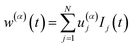
Let us consider a sample emitting fluorescence with two different lifetime signatures, so that the measured intensity signal Ij has the form
| | | Ij(t) = w(1)(t)p(1)j + w(2)(t)p(2)j | (1) |
where the index
j refers to the
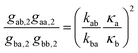
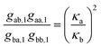
jth discrete
TCSPC time channel used for timing the
photon detection events with respect to the exciting laser pulses,
p(1,2)jare the
normalized fluorescence decay distributions over these channels for the two different fluorescence decay signatures of the sample (
e.g. two mono-exponential decays with different decay constant), and the
w(1,2)j) are the total intensities of both fluorescence contributions measured at a given time
t of the macroscopic time scale. When inspecting
eqn (1), it should be emphasized that two completely different times scales are involved: the macroscopic time scale of
t, on which the auto-correlation function (ACF) is calculated, and the (discrete) TCSPC time scale labelled by the numbers
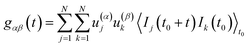
j of the corresponding TCSPC time-channel. Fluorescence decay-specific auto-(ACF) and cross-correlation (CCF) functions can now be defined by
| | | gαβ(t) = 〈w(α)(t0)w(β)(t0 + t)〉t0 | (2) |
where the
α,
β can take either the values 1 or 2, and the angular brackets denote averaging over time
t0. Please take into account that no reference to the TCSPC time scale is any longer present. The question now is how to extract the weights
w(α)(
t) from the measured
photon count data. Let us rewrite
eqn (1) in matrix notation as
where
I and
w are column vectors with elements
Ij and
w(α), respectively, and the elements of
matrix M are given by
Mjα =
pj(α). The most likely values of
w(α)(
t) at every moment
t are found by minimizing the quadratic form
24,25| | (I
−
![[M with combining macron]](https://www.rsc.org/images/entities/b_i_char_004d_0304.gif) w)T·V−1·(I
−
w) w)T·V−1·(I
−
w) | (4) |
where
is the average of
M over many excitation cycles, and
V is the covariance matrix given by
| | | V = 〈(I
−
w)·(I
−
w)T〉
−
〈(I
−
w)〉·〈(I
−
w)〉T = diag〈I〉 | (5) |
Here, the angular brackets denote averaging over an infinite measurement time interval of
t. In the last equation, it was assumed that the
photon detection obeys a Poissonian statistics so that 〈
IjIk〉
−
〈
Ij〉 =
δjk
〈
Ik〉. The solution of the above minimization task is given by using a weighted quasi-inverse matrix operation and has the explicit form
| | | w = [T·diag〈I〉−1·]−1·T·diag〈I〉−1·I = F·I. | (6) |
Thus,
u = [
T·diag〈
I〉
−1·
]
−1·
T·diag〈
I〉
−1 is the sought filter function that recovers
w(α)(
t) from the measured
Ij(
t),
| |  | (7) |
Notice that
u is a 2 ×
N matrix, with elements
uj(1,2), 1 ≤
j
≤
N, and a visualization of the meaning of the filter functions
uj(α) is depicted in
Fig. 1. Finally, the auto- and cross-correlations are calculated as
| |  | (8) |
The just described concept can be expanded to an arbitrary number of more than only two different fluorescence components in a straightforward way. It is often advisable to include, besides the distinct fluorescence contributions of the sample, an additional component with uniform distribution among the TCSPC diagram corresponding to uniform background (
e.g. dark counts, electronic noise,
detector afterpulsing). This automatically eliminates background contributions from the finally calculated fluorescence ACFs and CCFs, see
e.g. ref.
26.
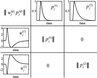 |
| | Fig. 1 Visualization of the meaning of the filter functions uj(1,2): At the top of the table, the fluorescence decay curves of the two states 1 and 2 are depicted. The filter functions, shown at the left side of the table, are designed in such a way that element-wise multiplication and summation of these functions with the fluorescence decay curves yields the identity matrix. In the table, we used the abbreviation . . | |
Four state model for the conformational and photophysical dynamics of a dye–protein complex
One of the most exciting applications of FLCS can be the study of molecular conformational changes of a biomolecule (protein, DNA, RNA etc.) that are reflected as lifetime changes of a fluorescence label. In the experimental example described in the next section, a fluorescing molecule is covalently attached to a protein, and one observes two distinct fluorescence decay times that supposedly reflect two different states of the protein–dye. In many cases, one has also to take into account fast photophysical processes of the fluorescent label itself, such as triplet state dynamics (intersystem crossing from the excited singlet state to the first triplet state with subsequent phosphorescence back to the singlet ground state) or conformational transitions between a fluorescent cis- and a non-fluorescent trans-state (as happens for many cyanine dyes).
Thus, we will consider the general case of a system depicted in Fig. 2: A dye-molecule complex undergoes major transitions between states A and B (from left to right and back in Fig. 2), whereas the dye itself makes transitions between a fluorescent (S) and a non-fluorescent (N) state (from top to bottom and back in Fig. 2). In the general case, the photophysical transition rate constants ksn and kns may themselves depend on whether the complex is in state A or B. Thus, the essential model parameters are the two transition rate constants kab and kba for the transition from A to B and from B to A, respectively, and the transition rate constants k(a)sn, k(b)sn, k(a)ns, and k(b)ns describing transitions of the label between a fluorescent and a non-fluorescent state. The rate constant of most interest are kab and kba, which may describe e.g. conformational changes of a protein or a DNA complex.
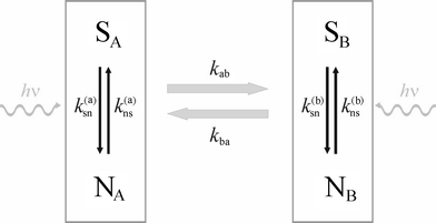 |
| | Fig. 2 Schematic of the four-state model for a dye–protein complex. The whole complex toggles back and forth between states A and B (left to right and back). In both states, the fluorescent dye can reside either in a fluorescent state S or a non-fluorescent state N. The fluorescent decay in states SA and SB is distinct and is used for FLCS. Transitions between fluorescent and non-fluorescent states may be light-driven (indicated by the wiggled lines with hν on top). | |
Let us denote the four probabilities to find the molecular complex in state SA, SB, NA, and NB by sa, sb, na, nb, respectively, which have all to take values between zero and one, all adding up to one. By introducing the column vector v = (sa, sb, na, nb)T, where the superscript T denotes transposition, the rate equations for the temporal evolution of these states are given by
| |  | (9) |
where the matrix
![[M with combining circumflex]](https://www.rsc.org/images/entities/b_i_char_004d_0302.gif)
has the explicit form
| | 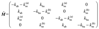 | (10) |
This linear system of differential equations can be solved in a standard way by finding the eigenvalues
λj and eigenvectors
êj of
matrix obeying the equation
êj =
λjêj. Then, the general solution for
v(
t) takes the form
| | 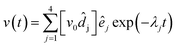 | (11) |
where the vectors
![[d with combining circumflex]](https://www.rsc.org/images/entities/b_i_char_0064_0302.gif) j
j form a conjugate basis to the eigenvectors
êj,
i.e. obey the relation
j·
êk =
δjk, and
v0 is the initial value of
v at
t = 0. Knowing this general solution of the rate equations, the
fast part of the ACFs and CCFs of the fluorescence emerging from states A and B are explicitly given by
| | 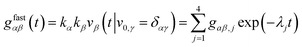 | (12) |
where the coefficients
gαβ,j have the form
| | gαβ,j = κακβ![[d with combining circumflex]](https://www.rsc.org/images/entities/i_char_0064_0302.gif) j,αêj,β j,αêj,β | (13) |
and
κα and
κβ are coefficients accounting for the relative brightness of the different fluorescent states. “Fast part” of the ACFs and CCFs means that one considers correlation lag times much shorter than the typical diffusion time so that one may assume that a molecule is not moving significantly within the spatially inhomogeneous molecule detection function, and the temporal dynamics of the ACFs and CCFs is dominated by the fast photophysical and molecular transitions.
For the matrix given in eqn (10), the eigenvalues are given by
| | 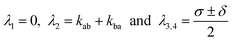 | (14) |
where the abbreviations
| | | σ = kab + kba + k(a)sn + k(a)ns + k(b)sn + k(b)ns | (15) |
and
| | | δ = {σ2
− 4[kba(k(a)sn + k(a)ns) + (k(b)sn + k(b)ns)(kab + k(a)sn + k(a)ns)]}1/2 | (16) |
where introduced. The zero value of the first eigenvalue,
λ1, reflects the conservation of the sum of all state occupancies (neglect of any photobleaching effects on the considered short time scale). The second eigenvalue,
λ2, is solely dominated by the transition dynamics between A and B, whereas
λ3,4 are determined also by the transitions between fluorescent and non-fluorescent state of the label. The quantities of interest are the transition rate constants
kab and
kba. The second eigenvalue
λ2 yields their sum; for separating this sum one can use the amplitude coefficients
gαβ,j from
eqn (12). After some tedious algebraic calculations one finds the two relations
| |  | (17) |
and
| |  | (18) |
allowing the determination of the brightness ratio
κa/
κb and, together with
eqn (14), the separate values of
kab and
kba.
Of course, for fitting experimentally obtained ACFs and CCFs one has also to consider the long-time behaviour of these functions that is determined by the diffusion of the molecules out of the detection volume. This can be done in a standard way by assuming a three-dimensional Gaussian profile of the molecule detection function leading to the complete result
| | 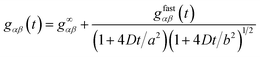 | (19) |
where
g∞αβ is a constant offset,
D is the diffusion coefficient, and
a and
b are the half-axes of the Gaussian profile perpendicular to and along the optical axis, respectively. For fitting purposes, it is also important to notice that all amplitude coefficients
gαβ,j are non-negative except
gab,2 and
gba,2 that are connected with the transition from A to B and back (and thus with
λ2) and generate rising terms in the CCFs. It should also be noted that the particular model used for describing the diffusional part of the ACFs and CCFs is unimportant because we are not interested in determining any diffusion coefficient by extracting rate constants acting on a much faster time scale.
Experimental application: conformational dynamics of a dye–protein complex
The experimental set-up was described in detail in ref. 23. The used excitation laser was a pulsed diode laser at 640 nm wavelength (PDL 800, PicoQuant) generating pulses with ca. 50 ps pulse width and 40 MHz repetition rate. The light of the laser was send through a single-mode glass fiber and subsequently collimated to form a beam with Gaussian beam profile of ca. 5 mm beam waist radius. The beam was then focused through an apochromatic water-immersion objective (1.2 N.A., 60×, Olympus) into the sample solution. Fluorescence is collected by the same objective (epi-fluorescence set-up), and then separated from the excitation light by a dichroic mirror (650 DRLP, Omega Optical). After passing two additional bandpass filters (670DF40, Omega Optical), a tube lens with 180 mm focal length focused it onto a circular pinhole with 100 µm diameter. After the pinhole, the light was split into two channels and refocused onto two single-photon avalanche diodes (SPAD) (SPCM AQR-13, Perkin Elmer). Fast electronics (TimeHarp 200, PicoQuant) was used for recording the detected photons in time-correlated time-tagged recording mode. From these raw data, the autocorrelation curves were calculated by cross-correlating photons from the two different SPADs. This cross-correlation prevented distortions of the autocorrelation curve due to SPAD afterpulsing.27
FCS measurements were performed on a ca. 10−9 M solution of Cy5–streptavidin (Molecular Probes) in bi-distilled water. FCS measurement times ranged between 20 min and 1.5 h, depending on the excitation intensity. The excitation power was measured with a power meter (S120 A, Thorlabs) at the back entry aperture of the objective. The power was adjusted with a gray filter wheel (STA-EAM 2, Laser 2000) and ranged between 1 and 400 µW for the diode laser. All measurements were performed at 20 °C.
Results and discussion
Measurements were performed at three different values of cw-excitation power, 80, 198, and 400 µW. Fig. 3 shows the TCSPC histogram obtained from one of these measurements showing the bi-exponential fluorescence decay of the measured fluorescence. The time region between the vertical lines was used for fitting a bi-exponential distribution to the measured curve (tail-fitting), and photons from this time window were also subsequently used for calculating the lifetime-specific ACFs and CCFs. The reason for limiting our analysis to this time window is the intensity-dependent shifting of the temporal response of the used SPADs: With increasing photon count rate, the temporal response of a SPAD can shift by more than half a nano-second to longer TCSPC times compared with its response at low photon count rates.
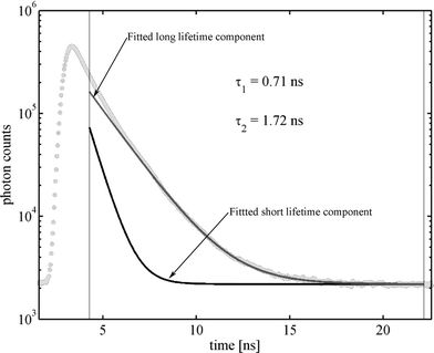 |
| | Fig. 3 Measured TCSPC curve for the Cy5–streptavidin complex (light grey dots). Black and dark grey lines are the fitted short and long lifetime components used as fluorescence decay patterns in the FLCS. The thin vertical lines delimit the time window used for the FLCS calculations. | |
That complicates the analysis of single molecules where huge fluctuations of photon count rate occur between times where no molecule is present within the detection volume and times where molecules diffuse through the detection volume. New generations of SPADs, so called PDMs (Microphoton Devices, Bolzano, Italy), do not show this kind of temporal response behaviour and will significantly improve FLCS data analysis, allowing to use photons over the whole TCSPC time range. Fig. 3 shows also the fitted mono-exponential contributions, having a fluorescence decay time of 0.71 and 1.72 ns, respectively. The two mono-exponential components of the fluorescence decay where taken as the separate fluorescence states A and B for which the ACFs and CCFs where calculated according to eqn (8) and using a dedicated algorithm for calculating correlation functions from asynchronous single photon counting data.28 In the FLCS calculations, we have taken a uniform TCSPC distribution as a third state for eliminating any background contributions from the fluorescence ACFs and CCFs. The obtained ACFs and CCFs for the long and short decay time fluorescence at an excitation power of 400 µW are depicted in Fig. 4. One can clearly see the rising components in the CCFs between the short decay time and long decay time fluorescence, being the result of a dynamic transition between the two states. For a static distribution of decay times, i.e. if a given molecule would never change its fluorescence decay time behaviour, no rising terms could occur in the CCFs. Next, we fitted the obtained ACFs and CCFs with a global fit of eqn (19) to all four ACFs and CCFs using the λj, gαβ,j and a/4D and b/4D as fit parameters. In these fits, the value λ1 was kept zero, and all gαβ,j where allowed to take only non-negative values except for gab,2 and gba,2 which were forced to adopt negative values, thus assuring that λ2 is indeed the eigenvalue equal to kab + kba. The obtained values of λ2, gαβ,1 and gαβ,2 where then used to calculate the rate constants kab and kba and as well as the ratio κa/κb using eqn (14), (17), and (18). The results for the three measurements at the excitation powers 80, 198, and 400 µW are shown in Fig. 5, together with a linear least-square fit of the obtained rate constants against the excitation power.
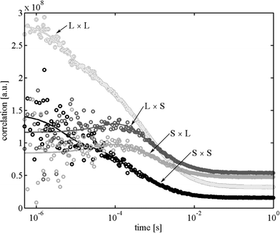 |
| | Fig. 4 Calculated (circles) and fitted (lines) ACFs and CCFs for the measurements at 400 µW excitation power. L denotes the long lifetime state, S the short lifetime state. The amplitude of the L × L auto-correlation is divided by a factor of ten for better comparability with the other curves. | |
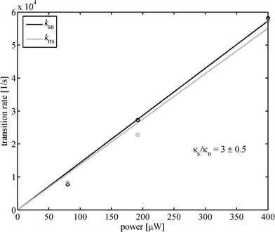 |
| | Fig. 5 Obtained values of the transition rate constants ksn and kns for the three excitation power values where FLCS measurements were performed. Solid lines show linear least-square fits. | |
As can be seen from Fig. 5, the obtained transition rates ksn and kns follow a linear relationship with excitation power, demonstrating that the transitions between the two observed lifetime states are light-driven. Moreover, the forward and backward rate constants are nearly equal, which is suspiciously similar to the measured dynamics of the conformational cis–trans-changes in free Cy5.29 In contrast to free Cy5, one has thus two fluorescing states that can be inter-converted by light and have both a lifetime different from the mono-exponential lifetime observed for free Cy5 (∼1 ns). Also, the FLCS curves cannot be satisfactorily fitted without taking into account the two additional exponential terms with λ2,3. This shows that, in contrast to free Cy5, the Cy5–streptavidin is a more complex multi-state system, with two fluorescing states and two non-fluorescing states. The light dependency of the transition rates indicates that the states are connected with the complex photophysics of Cy5 that is modified by the presence of streptavidin rather than with any conformational changes in the protein itself.
Conclusions
We have presented a thorough introduction into the theory and experimental application of FLCS. The analysis of the four-state model as given in the second part of the Theory section is quite general and applicable to many systems of practical interest. In particular, for many fluorescent labels the conformational state of the biomolecule influences the fluorescence lifetime, while the dye itself shows transition dynamics between fluorescent and non-fluorescent states (i.e. singlet/triplet states). We exemplified the principle working of the developed concepts on studying the transition dynamics between two fluorescent states with distinct lifetime in a Cy5–streptavidin complex. It is hoped that FLCS will find numerous applications in similar biophysical studies.
Acknowledgements
We are much obliged to Benjamin Kaupp for his generous support of our work.
References
- D. Magde, E. Elson and W. W. Webb, Phys. Rev. Lett., 1972, 29, 705–708 CrossRef CAS.
- E. L. Elson and D. Magde, Biopolymers, 1974, 13, 1–27 CrossRef CAS.
- D. Magde, E. Elson and W. W. Webb, Biopolymers, 1974, 13, 29–61 CrossRef CAS.
-
N. L. Thompson, in Topics in Fluorescence Spectroscopy, ed. J. R. Lakowicz, Plenum Press, New York, 1991, vol. 1, pp. 337–378 Search PubMed.
-
J. Widengren and Ü. Mets, in Single-Molecule Detection in Solution - Methods and Applications, ed. C. Zander, J. Enderlein and R. A. Keller, Wiley-VCH, Berlin, 2002, pp. 69–95 Search PubMed.
-
Fluorescence Correlation Spectroscopy, ed. R. Rigler and E. Elson, Springer, Berlin, 2001 Search PubMed.
- P. Schwille, Cell. Biochem. Biophys., 2001, 34, 383–408 Search PubMed.
- S. T. Hess, S. Huang, A. A. Heikal and W. W. Webb, Biochemistry, 2002, 41, 697–705 CrossRef CAS.
- O. Krichevsky and G. Bonnet, Rep. Prog. Phys., 2002, 65, 251–297 CrossRef CAS.
- P. Schwille, F. J. Meyer-Almes and R. Rigler, Dual-color fluorescence cross-correlation spectroscopy for multicomponent diffusional analysis in solution, Biophys. J., 1997, 72, 1878–1886 CrossRef CAS.
- J. Bieschke, A. Giese, W. Schulz-Schaeffer, I. Zerr, S. Poser, M. Eigen and H. Kretzschmar, Proc. Natl. Acad. Sci. U. S. A., 2000, 97, 5468–5473 CrossRef CAS.
- J. L. Swift, A. Carnini, T. E. S. Dahms and D. T. Cramb, J. Phys. Chem. B, 2004, 108, 11133–11138 CrossRef CAS.
- A. Camacho, K. Korn, M. Damond, J. F. Cajot, E. Litborn, B. H. Liao, P. Thyberg, H. Winter, A. Honegger, P. Gardellin and R. Rigler, J. Biotechnol., 2004, 107, 107–114 CrossRef CAS.
- K. Rippe, Biochemistry, 2000, 39, 2131–2139 CrossRef CAS.
- N. Baudendistel, G. Müller, W. Waldeck, P. Angel and J. Langowski, ChemPhysChem, 2005, 6, 984–990 CrossRef CAS.
- U. Kettling, A. Koltermann, P. Schwille and M. Eigen, Proc. Natl. Acad. Sci. U. S. A., 1998, 95, 1416–1420 CrossRef CAS.
- A. Koltermann, U. Kettling, J. Bieschke, T. Winkler and M. Eigen, Proc. Natl. Acad. Sci. U. S. A., 1998, 95, 1421–6 CrossRef CAS.
- K. Bacia, S. A. Kim and P. Schwille, Nat. Methods, 2006, 3, 83–89 CrossRef CAS.
- K. Heinze, A. Koltermann and P. Schwille, Proc. Natl. Acad. Sci. U. S. A., 2000, 97, 10377–10382 CrossRef CAS.
- L. C. Hwang and T. Wohland, J. Chem. Phys., 2005, 122, 114708 CrossRef.
- M. Böhmer, M. Wahl, H. J. Rahn, R. Erdmann and J. Enderlein, Chem. Phys. Lett., 2002, 353, 439–445 CrossRef CAS.
-
D. V. O'Connor and D. Phillips, Time-correlated single photon counting, Academic Press, London, 1984 Search PubMed.
- M. Böhmer, F. Pampaloni, M. Wahl, H. J. Rahn, R. Erdmann and J. Enderlein, Rev. Sci. Instrum., 2001, 72, 4145–4152 CrossRef CAS.
- G. Leclerc and J. J. Pireaux, J. Electron Spectrosc. Relat. Phenom., 1995, 71, 141–190 CrossRef CAS.
- J. Enderlein and R. Erdmann, Opt. Commun., 1997, 134, 371–378 CrossRef CAS.
- J. Enderlein and I. Gregor, Rev. Sci. Instrum., 2005, 76, 033102 CrossRef.
- M. Höbel and J. Ricka, Rev. Sci. Instrum., 1994, 65, 2326–2336 CrossRef.
- M. Wahl, I. Gregor, M. Patting and J. Enderlein, Opt. Express, 2003, 11, 3583–3591 Search PubMed.
- J. Widengren and P. Schwille, J. Phys. Chem. A, 2000, 104, 6416–6428 CrossRef CAS.
Footnote |
| † Edited by T. Gensch and C. Viappiani. This paper is derived from the lecture given at the X School of Pure and Applied Biophysics “Time-resolved spectroscopic methods in biophysics” (organized by the Italian Society of Pure and Applied Biophysics), held in Venice in January 2006. |
|
| This journal is © The Royal Society of Chemistry and Owner Societies 2007 |
Click here to see how this site uses Cookies. View our privacy policy here.