Consequences of chain networks on thermodynamic, dielectric and structural properties for liquid water
Teresa
Head-Gordon
a and
Steven W.
Rick
b
aDepartment of Bioengineering, University of California, Berkeley and Physical Biosciences Division, Lawrence Berkeley National Laboratory, Berkeley, California, 94720, USA
bDepartment of Chemistry, University of New Orleans, New Orleans, Louisiana, 70148
First published on 28th November 2006
Abstract
A vast array of experimental data on water provides a global view of the liquid that implicates its tetrahedral hydrogen-bonding network as the unifying molecular connection to its observed structural, thermodynamic, and dielectric property trends with temperature. Recently the classification of water as a tetrahedral liquid has been challenged based on X-ray absorption (XAS) experiments on liquid water (Ph. Wernet et al., Science, 2004, 304, 995), which have been interpreted to show a hydrogen-bonding network that replaces tetrahedral structure with chains or large rings of water molecules. We examine the consequences of tetrahedral vs. chain networks using three different modified water models that exhibit a local hydrogen bonding environment of two hydrogen bonds (2HB) and therefore networks of chains. Using these very differently parameterized models we evaluate their bulk densities, enthalpies of vaporization, heat capacities, isothermal compressibilities, thermal expansion coefficients, and dielectric constants, over the temperature range of 235–323 K. We also evaluate the entropy of the 2HB models at room temperature and whether such models support an ice Ih structure. All show poor agreement with experimentally measured thermodynamic and dielectric properties over the same temperature range, and behave similarly in most respects to normal liquids.
Introduction
There is a wealth of experimental data on water that probes structural, thermodynamic and dynamic properties over accessible regions of the phase diagram. Together these experiments provide a global view of the liquid that seems to emphasize its tetrahedral hydrogen-bonding network as the unifying molecular connection to these properties and ultimately to its anomalous features.1 Recently the classification of water as a tetrahedral liquid has been challenged based on X-ray absorption (XAS) experiments on liquid water.2 Wernet et al. interpret their experiments to involve a first coordination shell around a water molecule in the bulk fluid that has two hydrogen-bonding partners on average, resulting in a hydrogen-bonding network that replaces tetrahedral structure with chains or large rings of water molecules.2,3 To emphasize the boldness of this claim, it is still not established if the simplest anisotropic dipolar fluid model (a dipole embedded in a hard sphere), which also shows strong chaining in its network, even exhibits a liquid–gas phase transition.4Although such hydrogen-bonding patterns in water have been called into question based on inconsistencies with other structural measures of the liquid,5–13 there are yet other thermodynamic, dielectric, and dynamical experiments which are in themselves informative about the hydrogen-bonding network structure of liquid water in particular.14 The relevant summary of these experiments for the work described here is the existence of a temperature of maximum density (TMD), a negative thermal expansion coefficient below the TMD, a rapidly rising heat capacity at lower temperatures, a minimum in the isothermal compressibility that also rises sharply as temperature is lowered, a well-defined water molecule free energy in bulk, and a rather high dielectric constant when water is compared to other normal fluids. The question we address here is whether a tetrahedral network structure is necessary to exhibit these thermodynamic and dielectric trends with temperature, or is a hydrogen-bonded chain network capable of exhibiting the same water-like behavior?
This work explores three simulation models of liquid water that satisfies an average local environment in the liquid in which a water molecule participates in one strong donor and one strong acceptor hydrogen bond on average, based on the geometric criteria outlined for the local hydrogen-bonding environment in liquid water determined by XAS.2,15
 | (1) |
Simulation models and methods
Simulation model parameter constraints
It would seem that any new interpretation of water based on the structural condition of two hydrogen bonds using eqn (1) must also acknowledge at least a few additional fundamental physical constraints for viability of what is liquid water. One possible minimal set of additional constraints is that the condensed phase dipole moment is larger than the gas phase dipole moment, that the loss of hydrogen bonding does not result in a loss of too much binding energy, and that the model yields a liquid-like density. The use of a classical non-polarizable force field naturally assumes that hydrogen bonding in liquid water is strictly controlled by electrostatic interactions. Thus changes in charge magnitudes are the primary tuneable parameters for satisfying both an average of two hydrogen bonds per water molecule, a reasonable condensed phase dipole moment, and an acceptable liquid binding energy. Alterations of the Lennard-Jones parameters have the most impact on reproducing a reasonable water density at the state point of 298 K, 1 atm. Changes in water molecule geometry can be explored, but bond lengths of ∼1 Å and a bond angle of 104.5° are widely accepted values.For the purpose of the following discussion we define a quantity Δq = qH1 − qH2, where qH1 and qH2 are charge magnitudes of water’s hydrogens. Two of the water models examined here make the reasonable assumption that in order for one hydrogen to participate in hydrogen bonding while the other hydrogen does not, a distortion of the symmetric hydrogen electron density is required, i.e. Δq ≠ 0. Charge asymmetry is certainly a feature of polarizable models in which charge magnitudes fluctuate due to changing molecular environments (while maintaining charge neutrality). Fig. 1a shows the probability of observation of a given Δq for the TIP4P-FQ model in which it is seen that charge asymmetries as large as Δq = 0.3 e have a small but finite possibility. Very similar trends are observed in SPC-FQ and TIP4P-pol2. However in these polarizable models the charge asymmetries are transient in response to local symmetry-breaking environments, but when time or ensemble averaged yield a fluid with more than two hydrogen bonds per water molecule and with a most probable observation of Δq = 0.0. Fig. 1b shows the number of hydrogen bonds a water molecule has as a function of Δq. As the charge asymmetry grows, the number of hydrogen bonds per water molecule is seen to decrease by as much as 0.6, but the number of water molecules with significant reduction in hydrogen bond number is very small.
 | ||
| Fig. 1 (a) The probability of observation of Δq = qH1 − qH2 for the TIP4P-FQ, SPC-FQ and TIP4P-pol2 polarizable water models. (b) The average number of hydrogen bonds as a function of Δq = qH1 − qH2 for the TIP4P-FQ water model. | ||
One of the simulation models we examine was constructed by Soper to satisfy purely structural constraints, in the sense that it satisfies the 2HB criteria and is as consistent with both X-ray and neutron structure factors as possible.12 This asymmetric hydrogen charge model, based on parameter perturbations of the SPC/E model, yields ∼2.5 hydrogen bonds per water molecule and a liquid dipole moment of 3.03 D, and is described in more detail in the next section. Fig. 2 shows gOO(r) for the Soper asymmetric (SoperAsym) model, in which we see unusual sub-structure in the second peak that is evidence for the chain-like network structure advocated in ref. 2, and which we have shown is inconsistent with X-ray structural experiments.5 In addition, the SoperAsym model at the imposed liquid density yields a pressure of ∼10 000 atm, indicating that at ambient pressure it is supercritical liquid, or at least above the critical point of real water. This is perhaps not a surprising consequence of chain networks. It is thus evident that the SoperAsym model uses experimental structural constraints to bring tetrahedral structural signatures back into line, but requires the imposition of high pressure to yield a liquid-like density to do so.
 | ||
Fig. 2 Comparison of radial distribution functions for 2HB models from X-ray scattering experiments7 (—), SoperAsym (![[dash dash, graph caption]](https://www.rsc.org/images/entities/char_e091.gif) ), TIP4PAsym ( ), TIP4PAsym (![[dash dot, graph caption]](https://www.rsc.org/images/entities/char_e090.gif) ), and B60 (⋯). ), and B60 (⋯). | ||
We thus constructed a second model by perturbing the parameters of the TIP4P-EW16 model to satisfy the 2HB geometric criteria2,15 and to give a physically reasonable dipole moment, and also to yield a model with an accurate density and enthalpy of vaporization at 298 K, 1 atm. We tried developing it as a 2HB model that met the above minimal constraints while altering charge magnitudes on the hydrogen such that Δq = 0. However, never under the restriction of charge symmetry did we find a model with an intersection of both two hydrogen bonds per water molecule, an acceptable condensed phase dipole moment (>1.8 D) and adequate binding energy, while also having a typical water molecule geometry. Thus the best possible perturbed TIP4P-EW model also uses charge asymmetry to satisfy the 2HB criteria as advocated by Wernet and co-workers.2 The resulting TIP4PAsym model gives ∼2.2 hydrogen bonds per water molecule in the bulk and a condensed phase dipole moment of 2.43 D and has a reasonable density and enthalpy of vaporization at ambient T,P conditions. However the resulting liquid structure is clearly strongly perturbed as shown in Fig. 2, in which anti-tetrahedral signatures are seen in gOO(r) as a trough at ∼4.5 Å while chain networks are evident in the new peak at ∼5.6 Å. We also attempted to create a 2HB model based on the TIP5P-E model in two ways, first by adding charge asymmetry to the hydrogen centers and second by adding charge asymmetry to the lone pairs (which makes the water model chiral). Neither approach gave better properties than the TIP4PAsym model.
Independent of recent discrepancies with structural interpretations of liquid water,5–12 Lynden-Bell and co-workers have developed a series of families of artificial liquids whose intermolecular potentials differ from “real” water in a controlled way, to understand various pure water and aqueous solution properties.20–22 One artificial liquid is the bent family of models in which the network structure of the liquid changes from a three dimensional tetrahedral network to one-dimensional chains when the water molecule bond angle reaches 60°. The value of the Lennard-Jones σ parameter is changed to obtain the same number densities at 298 K and 1 atm pressure, while the ε parameters are unchanged. The B60 model has the same SPC/E charges, and thus the B60 model does have symmetry in the hydrogen charges such that Δq = 0. However in order to give the same SPC/E dipole moment the B60 bond lengths are reduced to ∼0.66 Å. Fig. 2 shows its gOO(r) in which the first peak moves inward and the second peak shifts outward as the bond angle decreases from tetrahedral. The variations in 3-body correlations reported in ref. 22 for the B60 liquid involves a network structure in which a B60 water molecule can make a double hydrogen bond to another molecule to form extended chains in three-dimensions. It satisfies the 2HB criteria, yielding a hydrogen-bond number of ∼2.2 per water molecule in the bulk.
Simulation models
Except for the simulation data shown in Fig. 1a and b, all of the simulation models used in this work are non-polarizable and based on the following potential energy description | (2) |
The first term in eqn (2) is due to Coulomb interactions
 | (3) |
 | (4) |
The Lennard-Jones description in the most general form of the models explored here is
 | (5) |
 | (6) |
For the TIP4PAsym model, S is a switching function defined by a polynomial in Z(r) = r2 − R2lower that describes a function in the range from Z = 0 (r = Rlower) to Z = R2upper − R2lower:
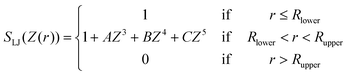 | (7) |
 | (8) |
The last term in eqn (2) is a potential energy term related to experimental structural constraints; it is only used in the SoperAsym model and is set to zero for the TIP4PAsym and B60 models. The constraints are experimental structure factors that are formulated as a potential of mean force using a computational technique known as the empirical potential structure refinement (EPSR).23,24 We refer the reader to details of the EPSR method in ref. 24.
Finally, the summary of water molecule geometries, charges, Lennard-Jones parameters for each of the water models are given in Table 1. We note that the SoperAsym model invokes a disorder in the OH bond lengths of a Gaussian form with a mean of 0.98 Å and standard deviation 0.074 Å. The SoperAsym also has disorder in the HOH bond angle, through a Gaussian distributed HH distances with average 1.56 Å and standard deviation 0.106 Å. The B60 and TIP4PAsym models have a fixed OH bond length of 0.6667 and 1.0 Å, respectively.
| Force field parameter | SoperAsym | TIP4PAsym | B60 |
|---|---|---|---|
| a Hydrogen bonds are disordered with an average hydrogen-bond length of 0.9572 Å. b The HH distances are disordered with an average length of 1.56 Å corresponding to an average HOH bond angle 105.5°. | |||
| r OH/Å | Variablea | 1.0 | 0.6667 |
| θ HOH/° | Variableb | 104.5 | 60.0 |
| d/Å | 0.000 | 0.125 | 0.000 |
| q H1/e− | 0.600 00 | 0.644 22 | 0.4238 |
| q H2/e− | 0.000 00 | 0.264 22 | 0.4238 |
| q O/e− | −0.600 00 | −0.908 44 | −0.8476 |
| ε O/kcal mol−1 | 0.139 82 | 0.362 75 | 0.154 90 |
| ε H/kcal mol−1 | 0.007 777 | 0.000 00 | 0.000 00 |
| σ O/Å | 3.166 | 3.05 | 2.92 |
| σ H/Å | 1.00 | 0.00 | 0.00 |
| Dipole moment/D | 3.03 | 2.44 | 2.35 |
| Q XX/D Å | −1.27 | −1.84 | −0.76 |
| Q YY/D Å | 1.36 | 1.92 | −0.08 |
| Q ZZ/D Å | −0.09 | −0.08 | 0.83 |
Simulation protocol
A cubic box with edge length of ∼24.8 Å was filled with 512 water molecules. Molecular dynamics (MD) simulations in an isothermal–isobaric (NPT) ensemble were performed using an in-house simulation program. The equations of motion were integrated using the velocity Verlet algorithm25 and with a time step size of 1 fs. The velocity update was done using only forces on real sites after forces on fictitious sites have been projected onto real sites. The duration of equilibration runs was 300 ps (T > 273 K) and 500 ps (T ≤ 248 K). Typical production runs were between 1.5 and 5.0 ns depending on temperature, and at least two MD runs per state point were completed. The intra-molecular geometry (rOH and θHOH) was constrained by applying the M_RATTLE algorithm16 using an absolute geometric tolerance of 10−10 Å. Temperature and pressure were controlled using Nosé–Hoover thermostats and barostats.26–28Coulomb interactions for the TIP4PAsym and B60 models were computed using the Ewald summation. For the computation of the reciprocal space sum, 10 reciprocal space vectors in each direction were used, with a spherical cutoff for the reciprocal space sum of n2x + n2y + n2z ≤ √105. The width of the screening Gaussian was 0.35 Å. The values of Rlower and Rupper for the switching function S we use in the simulations are 9.0 and 9.4 Å, respectively. The switching function in eqn (3) is also used as a molecule-based tapering function for the real-space Coulomb interaction energy in the Ewald sum, with a value of Rupper = 12 Å for the SoperAsym model.
Results
The three 2HB models have been characterized by computing bulk thermodynamic properties at 1 atm for the TIP4PAsym and B60 models and 10 000 atm for the SoperAsym model at 8 temperatures in the interval of 235–323 K. The results for the three models are summarized in Table 2 (SoperAsym), Table 3 (TIP4PAsym), and Table 4 (B60), and in Fig. 3–6 we plot the trends in thermodynamics and dielectric constants for each model against each other and against available experimental data.29–33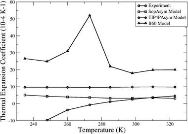 | ||
| Fig. 3 (a) Density dependence of 2HB models with temperature and (b) thermal expansion coefficient as a function of temperature. Experiment30 (circles), SoperAsym (squares), TIP4PAsym (diamonds), and B60 (triangles). | ||
 | ||
| Fig. 4 (a) Heats of vaporization of 2HB models with temperature and (b) constant pressure heat capacity as a function of temperature. Experiment30 (circles), SoperAsym (squares), TIP4PAsym (diamonds), and B60 (triangles). | ||
 | ||
| Fig. 5 Isothermal compressibility of 2HB models with temperature. Experiment30 (circles), SoperAsym (squares), TIP4PAsym (diamonds), and B60 (triangles). | ||
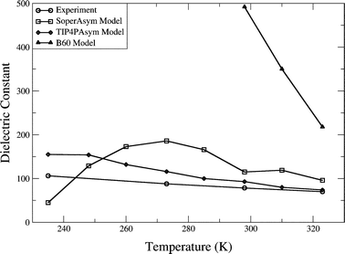 | ||
| Fig. 6 Dielectric constants of 2HB models with temperature. Experiment30 (circles), SoperAsym (squares), TIP4PAsym (diamonds), and B60 (triangles). | ||
| Property | SoperAsym model | |||||||
|---|---|---|---|---|---|---|---|---|
| Temperature/K | 235 | 248 | 260 | 273 | 285 | 298 | 310 | 323 |
| Duration/ns | 10.0 (5.0) | 7.0 | 6.0 | 4.0 | 3.5 | 3.0 | 2.9 | 2.9 |
| 〈ρ〉/g cm−3 | 1.024 (1.034) | 1.015 | 1.010 | 1.006 | 1.002 | 0.997 | 0.993 | 0.990 |
| 〈U〉/kcal mol−1 | −5675.0 (−5767.4) | −5589.4 | −5531.5 | −5475.9 | −5422.4 | −5366.5 | −5316.4 | −5260.6 |
| ΔHvap /kcal mol−1 | — | — | — | — | — | — | — | — |
| c p /cal mol−1 K−1 | 13.1 (153.8) | 10.9 | 10.2 | 10.0 | 9.5 | 9.6 | 9.9 | 9.5 |
| κ T /10−6 atm−1 | 25.1 (57.9) | 27.1 | 27.5 | 27.7 | 26.5 | 27.9 | 28.5 | 28.4 |
| α p /10−4 K−1 | 5.0 (76.7) | 4.3 | 3.9 | 3.6 | 3.1 | 3.2 | 3.5 | 3.1 |
| ε(0)/kcal mol−1 | 45 (63) | 129 | 173 | 186 | 166 | 115 | 119 | 96 |
| H-bond/molecule | 2.65 | 2.62 | 2.59 | 2.54 | 2.51 | 2.49 | 2.48 | 2.46 |
| Property | TIP4PAsym model | |||||||
|---|---|---|---|---|---|---|---|---|
| Temperature/K | 235 | 248 | 260 | 273 | 285 | 298 | 310 | 323 |
| Duration/ns | 10.0 | 7.0 | 6.0 | 5.0 | 3.5 | 3.0 | 2.9 | 2.9 |
| 〈ρ〉/g cm−3 | 1.059 | 1.046 | 1.034 | 1.021 | 1.009 | 0.996 | 0.984 | 0.971 |
| 〈U〉/kcal mol−1 | −6139.5 | −6066.3 | −5987.0 | −5922.3 | −5853.5 | −5778.5 | −5709.8 | −5634.5 |
| ΔHvap/kcal mol−1 | 12.248 | 12.128 | 12.013 | 11.890 | 11.777 | 11.653 | 11.541 | 11.417 |
| c p /cal mol−1 K−1 | 11.0 | 11.1 | 11.1 | 11.0 | 11.0 | 11.0 | 11.1 | 11.0 |
| κ T /10−6 atm−1 | 40.1 | 42.5 | 45.2 | 48.9 | 51.5 | 55.0 | 57.8 | 61.2 |
| α p /10−4 K−1 | 9.7 | 9.7 | 9.7 | 9.6 | 9.7 | 9.8 | 9.9 | 9.9 |
| ε(0)/kcal mol−1 | 155 | 154 | 132 | 116 | 100 | 93 | 80 | 74 |
| H-bond/molecule | 2.29 | 2.27 | 2.25 | 2.22 | 2.20 | 2.17 | 2.14 | 2.11 |
| Property | B60 model | |||||||
|---|---|---|---|---|---|---|---|---|
| Temperature/K | 235 | 248 | 260 | 273 | 285 | 298 | 310 | 323 |
| Duration/ns | 10.0 | 8.0 | 6.0 | 8.0 | 3.5 | 4.5 | 2.9 | 2.9 |
| 〈ρ〉/g cm−3 | 1.2275 | 1.1895 | 1.1535 | 1.0953 | 1.043 | 1.0163 | 0.992 | 0.966 |
| 〈U〉/kcal mol−1 | −4945.8 | −4837.7 | −4739.8 | −4599.9 | −4482.8 | −4408.8 | −4345.5 | −4276.2 |
| ΔHvap/kcal mol−1 | 9.945 | 9.754 | 9.567 | 9.323 | 9.108 | 8.983 | 8.878 | 8.763 |
| c p /cal mol−1 K−1 | 17.3 | 16.0 | 17.8 | 25.4 | 11.9 | 10.3 | 10.4 | 10.3 |
| κ T /10−6 atm−1 | 105.8 | 121.9 | 158.4 | 266.2 | 233.1 | 230.7 | 267.5 | 291.6 |
| α p /10−4 K−1 | 26.6 | 25.0 | 31.1 | 53.1 | 22.0 | 18.5 | 19.9 | 20.1 |
| ε(0)/kcal mol−1 | 3843 | 3866 | 4037 | 3493 | 907 | 492 | 350 | 218 |
| H-bond/molecule | 2.44 | 2.43 | 2.42 | 2.38 | 2.32 | 2.27 | 2.24 | 2.20 |
The average of the bulk density 〈ρ〉 is computed from the average volume of the simulation box 〈V〉
 | (9) |
Fig. 3a shows the temperature dependence of the density for the SoperAsym, B60 and TIP4PAsym models and experiment.29,30 No model shows evidence of a density maximum in the temperature profile, but instead shows a steady rise in density as temperature is lowered as is true for normal liquids. This is also manifest in the related thermodynamic quantity, the thermal expansion coefficient, αp, which we calculate using the enthalpy–volume fluctuation formula
 | (10) |
The enthalpy of vaporization ΔHvap is calculated from an NpT simulation as follows
 | (11) |
The isobaric heat capacity, cp, is computed by using the enthalpy fluctuation formula
 | (12) |
An additional thermodynamic quantity that shows unusual temperature dependence for water is the isothermal compressibility κT
 | (13) |
The final thermodynamic quantity we measure is the free energy to insert a water molecule into the bulk liquid, from which the entropy of the liquid can be found. The free energy change, ΔG, of a water molecule in the liquid relative to the gas phase is calculated using thermodynamic integration.34 We use 11–14 integration points, with separated-shifted scaling to eliminate singularities,35 along a path scaling in the interactions of a single water molecule with the others. The corresponding enthalpy change, ΔH, is found from ΔE + PΔV = −〈U〉/N + P〈V〉/N, where 〈U〉 and 〈V〉 are the average energy and volume of the liquid containing N molecules. The entropy change, ΔS, can be found using ΔS = (ΔH − ΔG)/T. These values are directly comparable to the experimental Ben-Naim and Marcus solvation free energies reported in ref. 32. Conventional water models are designed to reproduce 〈U〉 at 298 K, and they typically also get good agreement with experiment for ΔH and ΔS. For example, at 298 K and 1 atm, TIP3P gives ΔG = −6.18 ± 0.04 kcal mol−136 and TIP4P-FQ gives ΔG = −6.0 ± 0.4 kcal mol−1,37 close to the experimental value of −6.32 kcal mol−1.32
All three 2HB models show a range of free energy values (Table 5), ranging from larger or smaller entropy relative standard water models. The TIP4PAsym and B60 models have entropies that are higher than experiment, indicating more disorder as seems consistent with fewer hydrogen bonds relative to conventional water models. The SoperAsym model has a smaller entropy indicating more order, and the resulting positive ΔG shows that the liquid is thermodynamically unstable. Even though the SoperAsym model has fewer hydrogen bonds than conventional water models, the imposed (energetic) constraints to reproduce the partial pair correlation functions must be responsible for the smaller entropy value. If either of these constraints is relaxed, i.e. a model with two hydrogen bonds but inaccurate structure (like B60 or TIP4PAsym), or accurate pair correlation but with ∼3 hydrogen bonds, then the entropy will increase.
| ΔG/kcal mol−1 | ΔH/kcal mol−1 | −TΔS/kcal mol−1 | |
|---|---|---|---|
| TIP4PAsym | −8.33 ± 0.08 | −11.70 ± 0.01 | 3.37 ± 0.08 |
| SoperAsym | 1.24 ± 0.22 | −6.16 ± 0.01 | 7.40 ± 0.22 |
| B60 | −6.11 ± 0.07 | −8.56 ± 0.01 | 2.45 ± 0.07 |
| Experiment | −6.32 | −9.98 | 3.65 |
We also evaluate the static dielectric constant ε(0) using conducting boundary conditions
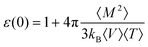 | (14) |
 | (15) |
The likely explanation of the observed unphysically large dielectric constants is the correlation with large dipole moments and small values of the diagonal of the quadrupole tensor.38Table 1 shows the evaluated dipole and quadrupole moments for each model. The dipole moments by design are not that different from standard water models, although for the asymmetric models, of course, the dipole direction will no longer be along the C2 axis. The quadrupoles are calculated relative to the center of mass, with the z-axis along the C2 direction, the x-axis out of the plane of the molecule, and the y-axis connecting the two hydrogen atoms. The three models all give values that are much less than the experimental gas-phase values for the quadropoles, consistent with the large dielectric constant of these models.38,39 For the B60 model, the quadrupole tensor is much different than experiment and other models, for which QXX ≈ −QYY and QZZ ≈ 0.37
The odd behavior of the dielectric constant collapsing to small values at low temperature in the SoperAsym model was further investigated with an additional 5.0 ns run to evaluate all properties. We found that the SoperAsym model exhibits some type of phase transition, characterized by a higher density and stronger binding energy (〈U〉) and rapidly rising values for all fluctuation properties (see values in parentheses for 235 K in Table 2). Again, the SoperAsym model appears to be metastable or unstable in this region of the phase diagram.
In order to evaluate the transferability of the 2HB models for characterizing other regions of the water phase diagram, simulations starting with an ice Ih lattice were performed. For all three models, it was found that at 273 K, the ice structure quickly melted to the liquid phase in less than 100 ps. The resulting phase has equivalent properties to that originating from the liquid (Tables 2–4). Thus the models are unable to form a stable ice Ih phase, as might be expected from a non-tetrahedral model.
Discussion and conclusions
The anomalous properties of water that are manifested in the stable region of the liquid include a temperature of maximum density, a negative thermal expansion coefficient at temperatures below the TMD, rapidly increasing heat capacity and isothermal compressibility, and a large and increasing dielectric constant as temperature declines, trends that are qualitatively different to other normal liquids. Recently, tetrahedral and translational metrics for quantifying structural order in water have been shown to correlate with liquid water’s unusual propensity for extremes in thermodynamic properties as the liquid is supercooled.1 One particularly strong structural correlate is a metric for tetrahedral network order.1The recent experimental XAS proposal2 that liquid water organizes into chain-like structure stands not only in direct conflict with other structural experiments,5–11 but should have been considered in the context of a broader array of experimental thermodynamic, dielectric, and dynamics data on liquid water. Water creates an open tetrahedral network due to its strong and directional hydrogen bonding, and this network structure has served as an important organizing principle for unifying much of that data into a global view of the water liquid.40 This global view of the liquid—beyond just structure—was the goal behind the development of the earliest ST2 model,41 and all subsequent models of liquid water.11,42,43 In spite of claims that the XAS findings showed serious discrepancies with structures based on current MD simulations,2 these simulation water models have continued to evolve to give better quantitative agreement with experiment outside of the regions for which they were parameterized. For example TIP4P-EW shows excellent agreement with liquid–vapor-phase equilibrium properties,44 exhibits ice Ih as the stable solid phase at the standard melting point,45 and gives excellent solvation free energies of small, nonpolar solutes.46 Whether a water model is successful at reproducing hydrophobic solvation free energies is strongly correlated with its ability to reproduce the experimental trends in water density.46
Thus when proposing any new structural organization for liquid water it is important to consider the global view of the liquid and whether it is sensible suggestion in the broader experimental context. Simulation models are perhaps the best way to examine this question, and as such we have developed three very differently parameterized 2HB models of water to ask the question: is an open chain network arising from reduced hydrogen bonding consistent with observed thermodynamic and dielectric trends of the water liquid? The purpose of the three very different methods of parameterization is to assume no single molecular reason for how 2HB chain networks form, and to see whether any common trends in thermodynamics or dielectric properties emerge from chain networks as a class of fluids.
None of the chain network models examined here exhibits a density anomaly when moving along its relevant isobar, and hence no chain model gives a negative thermal expansion coefficient over the observed temperature range of 235–323 K. All chain network models show a decreasing isothermal compressibility with decreasing temperature. These three properties and their trends with temperature are what are found for normal liquids, common substances that provide a reference for what is not water-like. The heat capacity trends for the TIP4PAsym model is in qualitative disagreement with experiment, while the B60 model shows quite unphysical temperature trends. The qualitatively water-like trends in heat capacity observed for the SoperAsym model is due to a high pressure phase transition since this water model is really a gas at 1 atm, and is a liquid at high pressure (∼10 000 atm). This is also evident from its positive free energy for water molecule insertion, indicating that the SoperAsym model is thermodynamically unstable. All models show much larger dielectric constants than real water, consistent with dielectric behavior of other chain forming fluids such as HF, and which likely arises from the reduction in the quadrupole tensor values which seems to be a consistent parameterization outcome for realizing a 2HB model. None of the chain network models explored here can support a stable hexagonal ice phase at 273 K.
With approximately the same number of adjustable parameters and functional forms for the system Hamiltonian, conventional water models yield water-like trends extending over the experimentally characterized phase diagram. The difference between the chain network models and these standard water models are parameters for the latter that promote additional hydrogen bonds and structural signatures such as experimentally plausible radial distribution functions or ring statistics consistent with tetrahedral network structure. While not an exhaustive study of parameter space for chain network models of water, the very different parameterization for the TIP4PAsym, SoperAsym, and B60 models to yield a set of 2HB models based on eqn (1) show surprising similarity in calculated thermodynamic and dielectric trends. The trends of 2HB models are clearly at odds with a large body of experimental and theoretical work done over many, many decades that classifies water as a tetrahedral liquid, and which differentiates it from other associative liquids that form non-tetrahedral networks.
Acknowledgements
THG gratefully acknowledges a Schlumberger Fellowship for support while on sabbatical at the University of Cambridge and financial support under the NSF-Cyber program. SWR would like to acknowledge support from NSF under contract number CHE-0213488 and from the Advanced Biomedical Computer Center at the National Cancer Institute. We thank Dr Alan Soper for supplying us with radial distribution functions and structure factors and full details of the SoperAsym model.References
- J. R. Errington and P. G. Debenedetti, Nature, 2001, 409, 318 CrossRef CAS.
- Ph. Wernet, D. Nordlund, U. Bergmann, M. Cavalleri, M. Odelius, H. Ogasawara, L. A. Naslund, T. K. Hirsch, L. Ojamae, P. Glatzel, L. G. M. Pettersson and A. Nilsson, Science, 2004, 304, 995 CrossRef CAS.
- M. Cavalleri, M. Odelius, D. Nordlund, A. Nilsson and L. G. M. Pettersson, Phys. Chem. Chem. Phys., 2005, 7, 2854 RSC.
- T. Tlusty and S. A. Safran, Science, 2000, 290, 1328 CrossRef CAS.
- T. Head-Gordon and M. E. Johnson, Proc. Natl. Acad. Sci. U. S. A., 2006, 103, 7973 CrossRef CAS.
- D. Prendergast and G. Galli, Phys. Rev. Lett., 2006, 96, 215502 CrossRef.
- J. D. Smith, C. D. Cappa, K. R. Wilson, B. M. Messer, R. C. Cohen and R. J. Saykally, Science, 2004, 306, 851 CrossRef CAS.
- (a) G. Hura, J. M. Sorensen, R. M. Glaeser and T. Head-Gordon, J. Chem. Phys., 2000, 113, 9140 CrossRef CAS; (b) J. M. Sorensen, G. Hura, R. M. Glaeser and T. Head-Gordon, J. Chem. Phys., 2000, 113, 9149 CrossRef CAS.
- A. K. Soper, Chem. Phys., 2000, 258, 121 CrossRef CAS.
- G. Hura, D. Russo, R. M. Glaeser, M. Krack, M. Parrinello and T. Head-Gordon, Phys. Chem. Chem. Phys., 2003, 5, 1981 RSC.
- T. Head-Gordon and G. Hura, Chem. Rev., 2002, 102, 2651 CrossRef CAS.
- A. K. Soper, J. Phys.: Condens. Matter, 2005, 17, 1 CrossRef.
- A. K. Soper, private communication of erratum preprint.
- P. G Debenedetti, J. Phys.: Condens. Matter, 2003, 15, R1669 CrossRef CAS.
- Y. A. Mantz, B. Chen and G. J. Martyna, Chem. Phys. Lett., 2005, 405, 294 CAS.
- H. W. Horn, W. C. Swope, J. W. Pitera, J. D. Madura, T. J. Dick, G. Hura and T. Head-Gordon, J. Chem. Phys., 2004, 120, 9665 CrossRef CAS.
- H. J. C. Berendsen, J. P. Grigera and T. P. Straatsma, J. Phys. Chem., 1987, 91, 6269 CrossRef CAS.
- S. W. Rick, S. Stuart and B. J. Berne, J. Chem. Phys., 1994, 101, 6141 CrossRef CAS.
- B. Chen, J. H. Xing and J. I. Siepmann, J. Phys. Chem. B, 2000, 104, 2415 CrossRef.
- D. L. Bergman and R. M. Lynden-Bell, Mol. Phys., 2001, 99, 1011 CrossRef CAS.
- R. M. Lynden-Bell and P. G. Debenedetti, J. Phys. Chem. B, 2005, 109, 6527 CrossRef CAS.
- R. M. Lynden-Bell and T. Head-Gordon, Mol. Phys., 2006 Search PubMed , in press.
- A. K. Soper, Chem. Phys., 1996, 202, 295 CrossRef CAS.
- A. K. Soper, Mol. Phys., 2001, 99, 1503 CrossRef CAS.
- H. C. Anderson, J. Comput. Phys., 1983, 52, 24 CrossRef CAS.
- S. Nosé, J. Chem. Phys., 1984, 81, 511 CrossRef CAS.
- W. G. Hoover, Phys. Rev. A, 1985, 31, 1695 CrossRef.
- G. J. Martyna, M. E. Tuckerman and M. L. Klein, J. Chem. Phys., 1992, 97, 2635 CrossRef.
- W. Wagner and A. Pruss, J. Phys. Chem. Ref. Data, 2003, 31, 387.
- G. S. Kell, J. Chem. Eng. Data, 1975, 20, 97 CrossRef CAS.
- D. G. Archer, J. Phys. Chem. B, 2000, 104, 8563 CrossRef CAS.
- A. Ben-Naim and Y. Marcus, J. Chem. Phys., 1984, 81, 2016 CrossRef CAS.
- D. P. Fernandez, A. R. H. Goodwin, E. W. Lemmon, J. M. Levelt Singers and R. C. Williams, J. Phys. Chem. Ref. Data, 1997, 26, 1125 CAS.
- D. L. Beveridge and F. M. DiCapua, Annu. Rev. Biophys., 1989, 18, 431 Search PubMed.
- M. Zacharias, T. P. Straatsma and J. A. McCammon, J. Chem. Phys., 1994, 100, 9025 CrossRef CAS.
- L. R. Olano and S. W. Rick, J. Am. Chem. Soc., 2004, 126, 7991 CrossRef.
- S. Sakane, E. M. Yezdimer, W. Liu, J. A. Barriocanal, D. J. Doren and R. H. Wood, J. Chem. Phys., 2000, 113, 2583 CrossRef CAS.
- S. L. Carnie and G. N. Patey, Mol. Phys., 1982, 47, 1129 CAS.
- S. W. Rick, J. Chem. Phys., 2004, 120, 6085 CrossRef CAS.
- C. A. Angell, R. D. Bressel, M. Hemmati, E. J. Sare and J. C. Tucker, Phys. Chem. Chem. Phys., 2000, 2, 1559 RSC.
- F. H. Stillinger and A. Rahman, J. Chem. Phys., 1974, 60, 1545 CrossRef CAS.
- W. L. Jorgensen and J. Tirado-Rives, Proc. Natl. Acad. Sci. U. S. A., 2005, 102, 6665 CrossRef CAS.
- A. Wallqvist and R. D. Mountain, Rev. Comput. Chem., 1999, 13, 183 Search PubMed.
- H. W. Horn, W. C. Swope and J. W. Pitera, J. Chem. Phys., 2005, 123, 194504 CrossRef.
- C. Vega, E. Sanz and J. L. F. Abascal, J. Chem. Phys., 2005, 122, 114507 CrossRef CAS.
- P. E. Krouskop, J. D. Madura, D. Paschek and A. Krukau, J. Chem. Phys., 2005, 124, 016012.
| This journal is © the Owner Societies 2007 |