Introductory lecture: Nonadiabatic effects in chemical dynamics
Ahren W.
Jasper
,
Chaoyuan
Zhu
,
Shikha
Nangia
and
Donald G.
Truhlar
Department of Chemistry and Supercomputing Institute, University of Minnesota, Minneapolis, MN 55455-0431, USA
First published on 15th July 2004
Abstract
Recent progress in the theoretical treatment of electronically nonadiabatic processes is discussed. First we discuss the generalized Born–Oppenheimer approximation, which identifies a subset of strongly coupled states, and the relative advantages and disadvantages of adiabatic and diabatic representations of the coupled surfaces and their interactions are considered. Ab initio diabatic representations that do not require tracking geometric phases or calculating singular nonadiabatic nuclear momentum coupling will be presented as one promising approach for characterizing the coupled electronic states of polyatomic photochemical systems. Such representations can be accomplished by methods based on functionals of the adiabatic electronic density matrix and the identification of reference orbitals for use in an overlap criterion. Next, four approaches to calculating or modeling electronically nonadiabatic dynamics are discussed: (1) accurate quantum mechanical scattering calculations, (2) approximate wave packet methods, (3) surface hopping, and (4) self-consistent-potential semiclassical approaches. The last two of these are particularly useful for polyatomic photochemistry, and recent refinements of these approaches will be discussed. For example, considerable progress has been achieved in making the surface hopping method more applicable to the study of systems with weakly coupled electronic states. This includes introducing uncertainty principle considerations to alleviate the problem of classically forbidden surface hops and the development of an efficient sampling algorithm for low-probability events. A topic whose central importance in a number of quantum mechanical fields is becoming more widely appreciated is the introduction of decoherence into the quantal degrees of freedom to account for the effect of the classical treatment on the other degrees of freedom, and we discuss how the introduction of such decoherence into a self-consistent-potential approximation leads to a reasonably accurate but very practical trajectory method for electronically nonadiabatic processes. Finally, the performances of several dynamical methods for Landau–Zener-type and Rosen–Zener–Demkov-type reactive scattering problems are compared.
1 Introduction
Electronically nonadiabatic processes (also called non-Born–Oppenheimer or non-BO processes) are defined as those in which the electronic state changes nonradiatively during the dynamical event. Electronically nonadiabatic processes are essential parts of visible and ultraviolet photochemistry, collisions of electronically excited species, chemiluminescent reactions, and many recombination reactions, heterolytic dissociations, and electron transfer processes. Often electronic excitation energies are much greater than the energies of nuclear motions, and electronically excited species have different valence properties than ground-state species; consequently electronically activated chemical systems may have dynamical mechanisms significantly different from those of thermally activated systems.The Born–Oppenheimer (BO) separation of electronic and nuclear motions and the use of classical mechanics to model the nuclear part of the problem have allowed for the development and successful application of a variety of theoretical electronic structure1 and dynamics2 methods designed for the electronically adiabatic case where the entire effect of the electronic subsystem is embedded in a potential energy surface that governs nuclear motion. The generalization of these theoretical methods to handle non-BO events adds new considerations and often significantly increases the computational demands of the calculation. From the point of view of the electronic subsystem, the computation of excited-state electronic wave functions and energies usually requires an open-shell formalism and expanded basis sets, and a consistent treatment of the active space is required in configuration interaction calculations.3–8 Furthermore, computing the couplings between the electronic states requires specialized methods, and the electronic couplings are singular, rapidly varying, high-dimensional vectors. From the point of view of the nuclear subsystem, the treatment is complicated by the need to consider a different potential energy surface for each electronic state and transitions between these surfaces.9 When conical intersections are present, nuclear motion on the adiabatic surfaces also involves geometric phases.10,11 Although great progress has been made in the quantum mechanical treatment of nuclear motion on coupled potential energy surfaces, the practical treatment of systems with a large number of nuclear degrees of freedom is greatly facilitated by using classical mechanics. Since the light mass and antisymmetry requirements of the electrons preclude a classical treatment, one then requires a semiclassical treatment that combines quantum mechanics for the electron motion with classical mechanics for the nuclear motion. A particularly subtle issue that reaches to the heart of the probabilistic interpretation of quantum mechanics12 (sometimes called quantum information theory or quantum measurement theory) is the loss of coherence in the quantal (electronic) subsystem due to its intersection with the classical subsystem (i.e., nuclear motion).13–15 In recent work, considerable progress has been made in sorting out these issues, and we can now present a more satisfactory theory than was possible a few years ago.
A brief theoretical discussion is presented in Section 2. In Sections 3–5, recent progress in the theoretical treatment of non-BO chemistry is discussed along three related lines: the calculation of potential energy surfaces and their couplings (Section 3), the development of methods for computing accurate quantum mechanical scattering dynamics (Section 4), and the testing, application, and systematic improvement of semiclassical methods for simulating non-BO dynamics (Section 5). Section 6 is a summary.
Although the specific examples considered in the present paper are processes initiated by collisions, the methods are general and can also be applied to unimolecular processes.
2 General theoretical considerations and definitions
The Hamiltonian for a molecular system may be writtenH(R,r)![[thin space (1/6-em)]](https://www.rsc.org/images/entities/char_2009.gif) =TR+He(R,r), =TR+He(R,r), | (1) |
Some chemical systems may be modeled adequately within the framework of the Born–Oppenheimer (BO) approximation.16–19 This approximation recognizes the large mass disparity of nuclei and electrons and allows their different-time-scale motions to be decoupled. Nuclear motion is then governed by a single BO potential energy surface V, which describes the variation of the ground-state electronic energy with changes in the nuclear geometry, i.e., the ground-state nuclear wave function ψ0 solves the equation,
| [TR+V(R)−E]ψ0(R)=0, | (2) |
| V(R)=〈ϕ0|He(R,r)|ϕ0〉r, | (3) |
For non-BO processes, more than one electronic state is important in the overall dynamics, and the single-surface treatment described by eqn. (2) is qualitatively incorrect. A proper theoretical framework may be developed in terms of a basis set of electronic wave functions ϕi, where i labels the electronic states, and optionally (but not necessarily) one may choose this basis so that ϕ0 has the same meaning as above. By analogy with the BO approximation, one may define potential energy surfaces for each electronic state, i.e.,
| Vii(R)=〈ϕi|He(R,r)|ϕi〉r, | (4) |
| Vij(R)=〈ϕi|He(R,r)|ϕj〉r. | (5) |
 | (6) |
 | (7) |
 | (8) |
 | (9) |
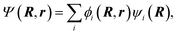
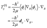
=j and i≠j) is often neglected. The matrix elements of the nuclear gradient operator dij are called nonadiabatic coupling vectors, and T(1)ijψj is called a nonadiabatic coupling term (NACT).
Eqn. (7) shows that nuclear motion in each electronic state is governed by the potential energy surface associated with that state as well as the various coupling terms in eqns. (5), (8), and (9). The situation may be simplified somewhat by making certain choices for the electronic basis. If the electronic basis is chosen such that Vij is diagonal, the nuclear motion is coupled only by the action of the nonadiabatic coupling terms in eqns. (8) and (9). This choice for the electronic basis is called the adiabatic18 electronic basis. Another choice for the electronic basis that is often useful is called the diabatic22–44 electronic basis. It is sometimes possible to rotate the electronic states in electronic state space (via a unitary transformation) to obtain a diabatic representation where the nonadiabatic couplings are small enough (for many purposes) to neglect. In the diabatic representation, the electronic Hamiltonian is no longer diagonal, and the nuclear motion is coupled by the diabatic or scalar coupling shown in eqn. (5). Alternatively, one can define or calculate approximate potentials in a diabatic representation and obtain the adiabatic representation by diagonalization of the potential energy matrix Vij, and in that case, if no approximations are made, the adiabatic and diabatic electronic representations yield identical results.
In general, an adiabatic-to-diabatic transformation that makes all of the components of dij zero is not possible.45,46 Useful diabatic representations may be developed that minimize these terms or—more generally—that make them small enough to be neglected, and these are often called quasidiabatic representations to emphasize the approximations involved, but we and many others call them diabatic with the understanding that strictly diabatic representations do not exist. It has been shown47 that in regions far from conical intersections, although one cannot make the NACTs zero, one can make their effect as negligibly small as for cases where the Born–Oppenheimer approximation is valid.
Finally, it is often possible to restrict theoretical attention to a subset of important electronic states which may be strongly coupled to one another but are only weakly coupled to all of the other electronic states. This procedure is called the generalized Born–Oppenheimer approximation.47,48
3 Coupled potential energy surfaces
In many theoretical treatments, the first step in modeling a non-BO system is the development of analytic expressions for the potential energy surfaces in eqn. (4) and their couplings. As discussed above, there are two possibilities for representing a set of coupled potential energy surfaces, the unique adiabatic representation or a nonunique diabatic one. They each have strengths and weaknesses. Some strengths of the adiabatic representation are that it is well defined, it lends itself well to using variational and perturbation theory methods to calculate it by electronic structure theory, it often provides a good zero-order picture when the coupling is neglected, and in principle it provides a basis for exact treatments. The diabatic picture, in contrast, inevitably neglects some coupling (because a “strict” diabatic basis does not exist) and is not unique, although it too sometimes provides a good zero-order picture when coupling is neglected. For large systems (organic photochemistry, photocatalysis, etc.) the rigor of the adiabatic representation is not so important, and in fact even for systems with 4–10 atoms, a rigorous treatment is usually not the goal. Therefore it may be very attractive to use a diabatic representation in which the coupling caused by the electronic Hamiltonian dominates the coupling due to nuclear kinetic energy so that the latter may be neglected for practical calculations.The diabatic representation has an important advantage that increases in attractiveness as systems get large, namely that the coupling is a scalar. For three coupled surfaces, there are three scalars, one coupling surface 1 to surface 2, another coupling 2 to 3, and the third coupling of 1 to 3. In contrast specifying the nonadiabatic coupling requires three 3N−6 dimensional vectors, where N is the number of atoms. Furthermore the diabatic surfaces and couplings are smooth, whereas the adiabatic surfaces have conical intersections and avoided crossings, and the nonadiabatic coupling is often rapidly varying and has singularities, and it requires special attention to consistent treatment of the origin49–52 and long-range effects.50,53,54
For these reasons there has been interest in developing practical methods for working with diabatic representations, and considerable progress was made in this direction. We particularly single out for discussion a new approach called the fourfold way.43,55,56 The fourfold way allows for the direct calculation of diabatic states and their couplings using the conventional variational and perturbational methods of quantum chemistry. This is particularly important because diabatic representations used for dynamics calculations should not be based on an arbitrary selection of configurations. Rather the variational principle should be used to optimize the space spanned by the strongly coupled electronic state vectors, then the electronic configuration space should be transformed to one that in some sense minimizes the nuclear momentum coupling, at least in regions where the nonadiabatic coupling is large. The fourfold way is designed to accomplish this process in a general way, but the method still requires care that is commensurate with the care required to treat ground-state problems by multi-configuration self-consistent-field methods, which can be chancy. This is not surprising because electronically nonadiabatic photochemistry intrinsically involves open-shell systems, and such systems do not lend themselves to black box approaches. The fourfold way has been developed for configurational wave functions based on complete active space multi-reference Møller–Plesset second order perturbation theory4 (CAS-MRMP2) and complete-active-space multi-configuration quasi-degenerate perturbation theory5 (CAS-MC-QDPT). The extension to the MC-QDPT version is particularly important because this is a perturb-then-diagonalize approach in which an effective Hamiltonian is formed by perturbation theory and then diagonalized. This allows the method to be valid for nearly degenerate states and even for truly degenerate states. (Isolated pathologies are possible6 but should not prevent useful applications of the method for dynamics.)
A key element in the fourfold way is that the diabatic systems are defined by a unitary transformation of ab initio adiabatic states, where the transformation36,43 is based on configurational uniformity. (Such a transformation has also been used fruitfully by other workers, based on other criteria.37,42) In order for this to produce useful diabatic states, it is necessary to first re-express the configuration state functions (CSFs) in terms of diabatic molecular orbitals (DMOs), and these are produced by the fourfold way. The essential step in using the fourfold way to obtain DMOs is maximizing a three-parameter functional that involves the sum of the squares of the orbital occupation numbers for all of the states, a state-averaged natural orbital term,38 and a transition density term. (The DMOs do not depend on tangentially related constructs such as one-electron properties.29) This threefold density criterion is often sufficient, but not in strong interaction regions for excitation from an open shell. In such regions we require the fourth element, which involves maximizing the overlap of one orbital with a reference molecular orbital. The fourfold way is effective at producing diabatic orbitals even in cases where a maximum overlap criterion35 applied to all orbitals fails. The resulting diabatic orbitals are globally defined and unique (path-independent) if the dominant configurations and weak coupling regions can be defined unambiguously. The method is general enough to allow for dominant CSF groups to have completely different members in different arrangements, and all ambiguities involving orbital and molecular orientation are solved by specific prescriptions or the introduction of resolution molecular orbitals.
Diabatic representations, with all their advantages for gas-phase processes, are also useful for condensed-phase photochemistry.44
Although these developments make the generation of diabatic representations more automatic, in some cases there may be practical advantages in working directly in the adiabatic representation because it altogether avoids the nonunique transformation to a diabatic representation. Ideally though, the choice between a diabatic and adiabatic representation should be based not on the convenience of generating the potential energy surfaces and their couplings, but rather on which one is more suitable for dynamics. Although accurate quantum dynamics are independent of representation, approximate methods usually depend on representation, and they will tend to be more accurate if one uses the representation with the smallest coupling between the surfaces; this is problem dependent and the best choice may also be method dependent. Thus two important questions emerge: (1) how can we determine, for a given system and a given approximate dynamics method, which representation will yield the most accurate results; (2) can we develop improved methods that are less dependent on representation than previously existing semiclassical methods? Both questions are addressed in Section 5.
4 Quantum mechanical dynamics
Once an analytic representation for the potential energy surfaces and their couplings is obtained (in either the adiabatic or diabatic representation), one may proceed to modeling or calculating the non-BO dynamics. Quantum mechanical calculations are especially challenging for non-BO systems both because there are open channels on more than one potential energy surface and also because, for typical energy gaps, the kinetic energy is high on at least one surface.For chemical systems with three or four atoms and two electronic states, the dynamics may be calculated using accurate quantum mechanical techniques. The method that we use to calculate accurate transition probabilities is time-independent quantum mechanical scattering theory. In these calculations we assume that a particular two-state diabatic representation of the potential energy surface is exact, and we neglect electronic angular momentum. After those two assumptions, the rest of the treatment is exact, that is, numerically converged to two or three significant figures. The calculations employ the outgoing wave variational principle57–61 (OWVP). The OWVP method, as we employ it, is particularly efficient because it divides the scattering problem into two smaller problems. The Schrödinger equation is solved by expanding the outgoing scattering waves in terms of internal-state channel functions for each asymptotic chemical arrangement. (A channel is defined by a set of quantum numbers, including the arrangement number, that characterizes the state of the completely dissociated reactant or product fragments.) The full Hamiltonian for each chemical arrangement is partitioned into a distortion Hamiltonian that contains some of the channel-channel coupling and causes rotationally-orbitally inelastic scattering and a coupling potential that contains the remainder of the channel-channel coupling. The solutions to the former are called distorted waves. The deviation of the accurate wave function from the distorted-waves is expanded in a basis set consisting of L2 functions and half-integrated distorted-wave Green's functions (HIGFs), and the deviation of the full scattering matrix from the part contributed by the distorted-waves is obtained by making it stationary with respect to variations of the coefficients of the L2 basis functions and the HIGFs. The L2 functions are sums of products of Gaussians, spherical harmonics, and diatomic eigenfunctions. The HIGFs are dynamically optimized by solving the distorted-wave problems on a finite difference grid as nonhomogenous coupled ordinary differential equations with two-point boundary conditions and with the quadrature grid for the matrix elements of the OWVP being a subgrid; this is more stable than forming the Green's functions from irregular solutions, and it avoids working with discontinuities or interpolation. Using this two-step scheme, the full scattering matrix is written as the sum of two terms, where the first term is the distorted-wave Born approximation for the scattering matrix obtained using the distorted-wave functions, and the second term is the contribution from the coupling potential.
The steps in the accurate calculations are therefore: (1) decouple the problem into small blocks in single chemical arrangements; (2) solve these multi-channel nonreactive problems to obtain partially coupled HIGFs; (3) calculate intra-arrangement and inter-arrangement matrix elements of the L2 basis functions and HIGFs; (4) solve a dense matrix problem for the coefficients of the L2 basis functions and HIGFs.
Several computational refinements are used to make the calculations efficient: (1) The grids used in the initial finite difference step are unevenly spaced so the subgrids used for later quadratures have efficient Gauss–Legendre node spacings. (2) High-order finite difference schemes are used. (3) The intra-arrangement integrals are re-calculated as needed to keep storage manageable (a so called “direct” algorithm). (4) The problem, including boundary conditions, is formulated in a molecule-fixed frame, which allows one to limit the basis set to small values of the body-frame angular momentum projections. (5) The problem is formulated with real boundary conditions and hence real arithmetic until the last step, where complex scattering matrix boundary conditions are used to avoid spurious singularities in the variational principle. (6) In calculating matrix elements, we prescreen both integrals and quadrature points to eliminate unnecessary work.
The OWVP method has been used to obtain fully-converged quantum mechanical scattering results for a variety of electronically nonadiabatic chemical systems. The initial such application was the nonreactive quenching process Na(3p)+H2→Na(3s)+H2 for zero62–65 and unit65 total angular momentum using a two-state representation of the NaH2 system. Accurate quantum mechanical calculations were also carried out66 for the spin–orbit-coupled collisions H+HBr→H2+Br(2P1/2) and H2+Br(2P3/2). The competition between electronically nonadiabatic reaction and electronic-to-vibrational energy transfer was investigated for the Br(2P1/2)+H2→HBr+H reaction.67 Calculations for a series of three-body model systems exhibiting avoided crossings in the vicinity of the reaction barrier showed strong nonadiabatic effects on reaction probabilities due to funnel resonances.68 OWVP calculations have been performed more recently on a variety of model systems, including three qualitatively different types of chemical systems: (1) systems with conical intersections,69–73
(2) systems with diabatic surfaces that cross and adiabatic surfaces that do not intersect,74 and (3) systems with wide regions of weak coupling where neither the diabatic nor the adiabatic surfaces cross.75,76 This set of calculations includes reactive69,72,74–76 and nonreactive71,72 scattering collisions as well as unimolecular excited-state decay processes.70,73
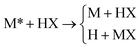
The availability of accurate quantum mechanical results for realistic full-dimensional non-BO systems allows for the systematic study of the accuracy of more approximate methods, and we have identified a subset of the calculations discussed above to serve as benchmark test cases. The systems are defined in the diabatic representation, and the set of diabatic surfaces (eqn. (4)) and their couplings (eqn. (5)) is referred to as a potential energy matrix or PEM. We include three Landau–Zener–Teller-type77–79 PEMs (collectively referred to as the MXH family74 of PEMs), which feature narrowly avoided crossings where the diabatic surfaces cross but the adiabatic surfaces do not. The three MXH PEMs differ from one another in the strength and width of their coupling, and all three MXH PEMs describe the reaction
 | (10) |
+HX or reactively to form H+MX. The masses of the M, X, and H atoms are 6.04695, 2.01565, and 1.00783 amu, respectively. The diabatic and adiabatic energies for one of the MXH systems along the collinear ground-state reaction path are plotted in Fig. 1(a). OWVP calculations with 20659 basis functions were carried out74 for all three MXH PEMs at total energies from 1.07 to 1.13 eV.
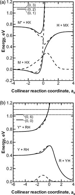 | ||
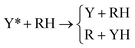
| Fig. 1 Adiabatic (solid lines) and diabatic (dashed lines) energies along the collinear ground-state reaction path for (a) one of the MXH systems and (b) one of the YRH systems. The total energies used in the quantum mechanical and semiclassical calculations are shown as dotted lines. The energies of the initial rovibrational states of the diatom used in the set of benchmark test cases are labeled (v, j), where v and j are the vibrational and rotational quantum numbers, respectively. Note: 1 a0=0.529 Å. | ||
The second family of PEMs included in the set of benchmark cases is the YRH family,75 which contains two Rosen–Zener–Demkov-type PEMs,80–82 featuring wide regions of weakly coupled and nearly parallel surfaces where neither the diabatic surfaces nor the adiabatic surfaces cross. The two YRH PEMs differ from one another in the strength of their coupling and describe the reaction
 | (11) |
Quantum mechanical results often display an oscillatory structure as a function of energy, whereas the approximate methods that we wish to test (which are based on classical theories) do not. In order to eliminate the effect of these oscillations when testing the approximate methods, we average the quantum mechanical results over several energies located around the nominal scattering energy. For the MXH systems, the quantum mechanical result at 1.10 eV was obtained by averaging results from 1.07 to 1.13 eV. Quantum mechanical results for the YRH systems were obtained at two energies: the 1.10 eV result was obtained by averaging results from 1.07 to 1.13 eV, and the 1.02 eV result was obtained by averaging results from 0.99 to 1.05 eV. The OWVP method gives the entire state-resolved scattering matrix, and in order to define a manageable test set, we include a subset of these transitions. Specifically, we consider the scattering dynamics of three initial rovibrational states for the diatom in the MXH systems, two initial rovibrational states for the diatom in the YRH systems at 1.1 eV total energy, and one initial rovibrational state for the diatom in the YRH systems at 1.02 eV total energy. The full set of benchmark quantum results includes 9 MXH cases, 3 YRH cases, and a total of 12 test cases with five different PEMs. The MXH and YRH systems have been used to systematically test several approximate methods, as discussed in the next section.
5 Semiclassical trajectory methods
For systems larger than a few atoms, an accurate quantum mechanical dynamical treatment is not computationally affordable. One must therefore rely on approximate “semiclassical” methods where the full dynamics of the system is approximated or simplified in some way using classical ideas.83 Although many semiclassical methods have been proposed and reviewed,21,48,84–87 few have been systematically tested against accurate quantum mechanical calculations for realistic, fully-dimensional chemical systems, due to the difficulty in obtaining quantum mechanical results. As discussed in Section 4, we have developed a broad test set of atom–diatom scattering calculations, and we focus our attention in this section on methods that have been validated using these test cases to determine their accuracy and applicability.The semiclassical methods considered here may be classified as trajectory ensemble methods, where a swarm of classical trajectories is used to simulate the nuclear motion of the system. A quantum mechanical nuclear wave packet has some inherent width in configuration and momentum space, whereas classical trajectories are delta functions in phase space. (Equivalently, a quantal particle's coordinates and momenta have some inherent uncertainty or spread, whereas in a classical system these quantities are fully determined.) An ensemble of trajectories is therefore required to approximate the quantal situation, where the distribution of the trajectories in the ensemble mimics the width of the accurate quantal wave packet.87
Trajectory ensemble methods may be further categorized into those in which the entire ensemble of trajectories is treated simultaneously and trajectories are allowed to influence each other's motions (coupled trajectory methods), and those in which each trajectory in the ensemble is treated independently (independent trajectory methods). Several coupled-trajectory methods have been developed.88–99 Some involve “dressing” a classical trajectory with a shape functions such as a Gaussian, and using the overlap of these shape functions to determine the overall dynamics of the system, and others involve using trajectory-derived ensemble-averaged quantities in the equations of motion.
We note that some of the coupled-trajectory methods are very similar to Gaussian wave packet methods in which the centers of the Gaussians follow classical trajectories. These methods are based on early work by Heller.100,101 One method that has been systematically tested is the minimal version102 of the full multiple spawning method103,104 (FMS-M). In this method, a number of Gaussian-shaped packets are propagated along classical trajectories, and the trajectories occasionally spawn new wave packets, which propagate on other electronic surfaces. Electronic state density is allowed to flow back and forth between the packets, thus simulating the non-BO event. This method strikes a nice balance between including quantum mechanical effects and maintaining computational efficiency, but because one cannot afford to spawn a complete basis set of wave packets moving in all directions, and because one usually makes approximations that force the wave packet centers to follow classical-like paths, the method does not eliminate some of the arbitrariness (see below) that is most troubling in more classical approaches. Furthermore the propagation of a wave packet is more expensive than the propagation of a trajectory, and, as with all wave packet methods, one must be careful to fully sample phase space, a drawback which significantly raises the cost of wave packet methods for large systems.
Another class of wave packet methods is based on the time-dependent multi-configuration time-dependent Hartree method.105,106 These methods are viewed as approximate quantal methods rather than semiclassical methods and will not be discussed here. Coupled-trajectory methods and multiple spawning methods may be used to study the importance of coherent motions, but their computational cost is higher than independent trajectory methods for full-dimensional systems. We will focus our attention on independent-trajectory methods.
A non-BO process modeled using classical trajectories may be described as follows: as the ensemble of nuclear trajectories evolves in time, the nuclear motion causes a change in the overall electronic state of the system (via the nonadiabatic vector momentum (and possibly kinetic energy) couplings or diabatic scalar potential coupling terms) which in turn results in a new effective potential energy felt by the trajectories, affecting the nuclear motion. This nuclear-electronic interaction is the source of nonadiabatic electronic state changes, and to properly treat these non-BO effects a self-consistent treatment of the nuclear-electronic coupling is necessary (i.e., the electronic and nuclear degrees of freedom must be made to evolve simultaneously). Several methods for modeling this self-consistency within the independent-trajectory approximation have been proposed, and we discuss them next.
The electronic motion along each classical trajectory is obtained by propagating the solution to the electronic Schrödinger equation with the appropriate initial conditions. The solution may be represented in the form of an electronic density matrix ρ, where the diagonal element ρii is the electronic state probability for state i, and ρij for i≠j are the electronic state coherences.21,107 If the entire system is described in quantum mechanical language, then ρ is the reduced density matrix obtained by tracing the density matrix of the entire system (electrons and nuclei) over the nuclear degrees of freedom. The Schrödinger equation for the wave function reduces (neglecting T(2)ij) to the following equation for the reduced density matrix:85
 | (12) |
| Fij≡Vij−iℏṘ·dij | (13) |
One may anticipate that a successful semiclassical effective potential energy function VSC will be some function of the potential surfaces, their couplings, and ρ. As discussed above, one can express the electronic potential energies and their couplings in either the adiabatic or diabatic representations, and these two representations are equivalent if no approximations are made. Several of the semiclassical methods that will be discussed next involve approximations that do not preserve representation independence, and one must choose which representation to use for a given simulation. When this is the case, we will discuss a method for choosing the preferred representation. However, for some non-BO problems it may not be possible to assign a single preferred electronic representation. For example, a system may have two or more distinct dynamical regions which differ in their preferred representation. Therefore, it is desirable to develop semiclassical methods that are accurate in both the diabatic and adiabatic electronic representations.
Several semiclassical algorithms have been proposed with differing prescriptions for VSC, and the approaches may be divided into two general categories: (1) time-dependent self-consistent-potential methods, and (2) trajectory surface hopping methods. Each category will be discussed briefly.
Semiclassical time-dependent self-consistent-field (TDSCF) theory provides a general framework for incorporating quantum mechanical effects into molecular dynamics simulations. The semiclassical TDSCF method is also known as the semiclassical Ehrenfest (SE) method, the partially classical Ehrenfest model,108 the time-dependent Hartree method, the time-dependent self-consistent field method,9,108,109 the self-consistent eikonal treatment,110 the hemiquantal method,111 and mean-field theory. In this article we are especially concerned with the use of this method to treat the problem of vibronic effects, that is, the coupling of electronic and nuclear motions when the Born–Oppenheimer approximation breaks down. We group all methods of this type into a general category that we call self-consistent potential methods. The Ehrenfest method converts this problem to classical molecular dynamics on a time-dependent average potential energy surface that is most appropriate for strong interaction regions but leaves the system in an unphysical final state that corresponds to a quantum superposition of pure states. It is well known that an open quantum system, that is a quantum system interacting with an environment (a “bath”), tends to a statistical mixture112 of final states, not a pure state corresponding to a quantal superposition of final states. The quantum mechanical description of this phenomenon is that the off-diagonal elements (which are called coherences) of the reduced density matrix tend to zero. The zeroing of the off-diagonal elements of the density matrix goes by many names including decoherence, transverse or spin–lattice relation, and reduction of the wave packet. This general phenomenon has specific relevance to the present problem because the electronic degrees of freedom may be considered to be an open quantum system in the presence of the bath of nuclear degrees of freedom. Thus the nuclear degrees of freedom decohere the electronic density matrix, and this occurs continuously at a finite rate, not suddenly at a surface hop or a detector. When the coherences (i.e., the off-diagonal elements of ρ) decay, the system becomes a statistical mixture, not a pure state. The system should then evolve like a mixture of systems on the different potential surfaces, and the self-consistent potential for the ensemble of trajectories is then an average of the various potential surfaces. This is where the Ehrenfest method fails because it evolves each trajectory on an average potential (which is different for each trajectory) rather than averaging the evolutions on the individual surfaces. We need to introduce an algorithmic decay of mixing by which the electronic density matrices generating the potential energy surfaces for the individual trajectories each lose their mixed character and become a pure state; this decay of mixing must be stochastic or probabilistic such that the fraction of trajectories propagating on each pure surface is equal, on average, to the probability of observing each pure state in the statistical mixture corresponding to the reduced density matrix. Furthermore not only must the nuclear motion be consistent with the electronic density matrix, but also the electronic density matrix is a function of the nuclear trajectory; that is, the theory must be self-consistent. This is the physical picture behind the coherent switching decay of mixing113
(CSDM) algorithm and the earlier self-consistent decay of mixing114
(SCDM) algorithm. These algorithms introduce continuous decoherence toward a pure state, called the decoherent state, and this pure state is stochastically switched from one to another state in a self-consistent114 or coherent113 way along the trajectory. In both algorithms the effective potential for nuclear motion is obtained from the self-consistent electronic density matrix, and in the SCDM this self-consistent density matrix also governs the switching of the decoherent state. However, we have found that for some problems the evolution of the electronic density matrix that governs the switching should be more coherent than the evolution of the electronic density matrix that governs the effective potential for nuclear motion, and making this switching coherent for each complete passage of a region of strong interaction of the electronic states makes the CSDM algorithm113 more accurate than the earlier114 less coherent algorithm. The switching is not completely coherent throughout the trajectory but rather coherent during each complete passage of the system through a region of strong interaction of the electronic states. At a point of minimum interaction of the electronic states, between strong coupling regions, the electronic density matrix (![[small rho, Greek, tilde]](https://www.rsc.org/images/entities/b_i_char_e0e4.gif) ) that governs the switching is re-set to the one (ρ) that governs nuclear motion.
) that governs the switching is re-set to the one (ρ) that governs nuclear motion.
But toward which pure states should the systems decohere, e.g., toward the adiabatic pure states or the diabatic ones? What is the privileged electronic basis in which the density matrix becomes diagonal? The analog of this question in quantal measurement theory is: what is being measured?115 This is clearly determined by the measuring system, which from the point of view of the quantum system, is the environment. In our problem, the environment is the nuclear degrees of freedom. In quantal measurement theory, the privileged basis selected by the environment is called the pointer basis,115 and it is determined by the interaction Hamiltonian connecting the two subsystems. In the special case where the environment changes slowly on the natural time scale of the quantal system, the pointer basis becomes the adiabatic basis of the quantal system,116i.e., it is determined by the quantal system's internal Hamiltonian, not by the system-environment coupling. Thus for systems where the Born–Oppenheimer approximation is a good zero-order description, the adiabatic basis should be the decoherent basis. However, we are interested in systems with strong interactions between the states, i.e., Born–Oppenheimer breakdown, and in such cases it is not easy to determine the pointer basis, although our physical intuition tells us that when the diabatic representation is a good zero-order approximation, the diabatic basis should be the decoherent basis. One problem though is that the pointer basis may be different at different geometries. A key to resolving the dilemma of how to choose the decoherent basis is provided by recalling that the exact quantum mechanical solution is independent of the basis in which the problem is solved. Therefore we seek a method that gives similar results in the two extreme bases, adiabatic and diabatic. Then the choice of decoherent basis will not be so much of a problem because one will get an accurate answer even if one locally makes the wrong choice.
The starting point for mean-field methods is the quantum Ehrenfest theorem117,118 which states that the expectation values of the position and momentum operators evolve according to classical equations of motion with an effective potential energy function given by the expectation value of the potential energy operator. We define the semiclassical Ehrenfest (SE) independent-trajectory method by taking VSC to be the expectation value of the electronic Hamiltonian:9,48,119
 | (14) |
The SE method has the desirable feature that it is formally independent of electronic representation.119 Unfortunately, the SE method has many more disadvantages that result from the mean-field assumption.86 At any instant along an SE trajectory it is physically meaningful for the nuclear motion of a system to be influenced by some average of the potential energies of all of the electronic states. However, it is not physically meaningful for the nuclear motion corresponding to each electronic state to be described by a single trajectory. If the potential energies of the various electronic states are similar in topography and energy, then the nuclear motions in each state will be such that an average SE trajectory may provide a reasonable approximation. For many chemical systems, however, this is not the case, and it is not possible for a mean-field trajectory to accurately approximate the motion in these different electronic states. An important consequence of this arises in the case of low-probability events. An SE trajectory will be dominated by the character of the high-probability motions, and low-probability motions may not be properly explored. Furthermore, it is not clear how to interpret the final state of an SE trajectory. In general, an SE trajectory will finish the simulation in a coherent superposition of electronic states, whereas physically one expects isolated products to be in pure electronic states (if there is no electronic state coupling in the product region of phase space). The internal energy distribution of products in a superposition of electronic states is not reliable because it does not correspond directly to the internal energy distribution of any single physically meaningful product.
The SCDM114 and CSDM113 methods, introduced above, are modified SE methods that force the system into a pure electronic state as the system passes through and leaves the strong coupling region. Both methods add decay terms to off-diagonal matrix elements of the electronic density matrix ρ such that the system decoheres (demixes) to a pure electronic state K in regions of vanishing coupling. These decoherence terms generate a force, called the decoherent force, on the nuclear coordinates, and the direction of the force determines which system degrees of freedom gain or lose energy due to the decoherent force. Since the CSDM method appears to be accurate for a wider class of cases, we will focus on CSDM. In the CSDM method, the decoherent force is in the direction of a unit vector ŝ; for large d, ŝ is parallel or antiparallel to d, as motivated by semiclassical arguments120,121 and tests against accurate quantal results;70 and for small d, ŝ is parallel or antiparallel to the vibrational momentum Pvib. The first order rate constant governing decoherence of the coherence of states i and K is 1/τiK, where τiK is a decoherence time (or demixing time) given in terms of a pure dephasing time τPDiK by
| τiK=τPDiK(1+S) | (15) |
 | (16) |
 | (17) |
It is important to emphasize that eqn. (15) is the time constant for algorithmic decay of mixing, not for physical decoherence. The use of S>0 allows for the difference. We have found that the balance of coherence and decoherence in the algorithm is critical and one can make up, to a certain extent, for too much decoherence by increasing τiK.113 For many cases the results are not very sensitive to E0 in the range around E0=0.1 hartree and so we use that value here. In light of these considerations it is interesting to briefly consider the physical origins of decoherence.
A useful semiclassical analysis of decoherence has been provided by Feite and Heller.122 They identified three contributions to decoherence in general, but in the case of electronically nonadiabatic molecular processes, one needs to consider only two: bath overlap decay and pure dephasing due to averaging over a distribution of phases associated with different semiclassical trajectories. Eqn. (15) includes the pure dephasing contribution but not the bath overlap decay contribution. In the present case the bath consists of the nuclear degrees of freedom, and the nuclear overlap decay has been emphasized by Prezhdo and Rossky,13 who describe it as the nonradiative analog to Franck–Condon overlap factors123 in radiative processes. To include these effects in the ideal case of first order decay of decoherence we would replace τPD by τD where
 | (18) |
A CSDM trajectory behaves like an SE trajectory in strong coupling regions and collapses to a pure state asymptotically. The method retains the desirable features of the SE method in that the coherences between electronic states are included and the motion is independent of representation when the electronic states are strongly coupled. Additionally, the CSDM method is able to treat low-probability events and gives realistic product states.
As discussed above, a semiclassical trajectory calculation involves computing an ensemble of trajectories and averaging the results. In order to highlight the differences between the SE and CSDM methods, however, we consider a single representative trajectory for each method, as shown in Fig. 2. These trajectories were taken from a scattering calculation using an MXH PEM. In Fig. 2, the population P2
(=ρ22) of the excited electronic state is shown, along with the three internuclear bond distances, as functions of time. The SE trajectory (Fig. 2(a)) finishes the simulation in a coherent superposition of electronic states with P2≈0.7. This leads to an unphysical internal energy for the product fragment corresponding to neither the M*+HX nor the M+HX molecular arrangements, as discussed above. Furthermore, the excited state in the H+MX asymptote is very high in energy, and even a small about of mixing in of the excited state turns the trajectory away from the H+MX asymptote (this dynamical feature may be seen in Fig. 2(a) at ∼0.23 ps).
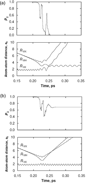 | ||
| Fig. 2 Representative trajectories for the M+XH system in the adiabatic representation for the (a) SE and (b) CSDM methods. The potential energy matrix is the SB one,74 the total energy is 1.10 eV, and the initial vibrational-rotational state is v=j=0. The excited state population P2 and internuclear bond distances RAB are shown as functions of time. | ||
A CSDM trajectory for the same set of initial conditions is shown in Fig. 2(b). The behavior of the CSDM trajectory is very similar to the SE trajectory for the first half of the trajectory. With the CSDM method, however, the system starts to exit the H+MX asymptote with P2≈0.0 and is therefore able to proceed to form H+MX products. For this test case, the accurate quantum mechanical probability of reaction is 0.15, which agrees much better with the CSDM method (0.16) than with the SE method (0.03).
Another approach to independent-trajectory dynamics is the trajectory surface-hopping approach,21,48 where the semiclassical potential VSC is taken to be the potential energy surface that corresponds to the currently occupied state, i.e.,
| VSC=Vii. | (19) |
The surface hopping method that has the most elegant derivation is the molecular dynamics with quantum transitions method of Tully;21,107 we call this Tully's fewest-switches (TFS) method. Trajectories are propagated locally under the influence of a single-state potential energy function, and this propagation is interrupted at small time intervals with hopping decisions. A hopping decision consists of computing a probability for hopping from the currently occupied state to some other state such that hopping only occurs when there is a net flow (in an ensemble-averaged sense) of electronic state probability density out of the currently occupied state; this gives the fewest hops consistent with maintaining self-consistency. At each hopping decision, the hopping probability is computed and compared with a random number to determine if a surface hop occurs. The non-BO event is represented as a swarm of TFS trajectories, each hopping between the various electronic states at slightly different locations. In this way, the flow of probability density (which may occur over an extended region in phase space) is accurately modeled.
The surface hopping method, because it involves discrete electronic transitions, provides a particularly convenient way to decide whether the adiabatic or diabatic representation provides a better zero-order picture for a given system. We have previously described a criterion (called the Calaveras County (CC) criterion73,86) for determining in the absence of quantum mechanical data which representation is likely to be more accurate. Specifically, the CC representation is defined as the representation in which the number of attempted surface hops is minimized, as estimated from a small set of TFS calculations, i.e., the CC representation is the representation in which the system is the least dynamically coupled.
A significant problem that must be dealt with when using the TFS formulation (and many other surface hopping schemes) is the existence of classically forbidden electronic transitions.75 The TFS algorithm may predict a nonzero hopping probability to a higher-energy electronic state in regions where the nuclear momentum is insufficient to allow for an energy adjustment that will conserve total energy. For example, due to tunneling, quantum mechanical particles have some probability density in regions of phase space that are classically forbidden. These tails of the nuclear wave function decrease exponentially, so we do not expect significant populations in “highly” classically forbidden regions, but these tails may be important for regions that are only “slightly” classically forbidden, i.e., regions that are somewhat close to classically accessible regions. An accurate treatment of classically forbidden transitions associated with these tails may be important for some problems.
In the original implementation of the TFS algorithm, the method was applied to simple one-dimensional problems where frustrated hopping was not important. When frustrated hops were encountered, however, either the attempted hop was ignored,107 or the nuclear momentum was reflected along the nonadiabatic coupling vector, that is, classically forbidden (or “frustrated”) hops were treated by reversing the nuclear momentum in the direction of the nonadiabatic coupling vector dij and continuing the trajectory without a surface switch.125,126 This latter prescription, which elsewhere75 we have called the “−” prescription, is motivated by interpreting the frustrated hopping event as the trajectory being reflected by a change from one surface to another along a hopping seam normal to the nonadiabatic transition vector (i.e., in the direction of dij). Müller and Stock, however, advocated127 that frustrated hops should be ignored, and we call this the “+” prescription.
The + and − prescriptions have been tested numerically,75,128 and it was shown that the − prescription is systematically more accurate for computing branching probabilities, whereas the + prescription gives more accurate internal energy distributions. It is therefore natural to attempt to combine the + and − approaches, and the ▽V prescription129 is one such attempt. Specifically, if at a frustrated hop the force associated with the potential energy of the target electronic state in the direction of dij has the same sign as the nuclear momentum along dij, then the + prescription is used. Otherwise, the − prescription is used. In either case, no surface hop occurs. Using the ▽V prescription, the trajectory instantaneously “feels” the force associated with the target electronic state and is “accelerated” (which is equivalent to ignoring the surface hop due to the enforcement of energy conservation) or reflected accordingly. It has been shown numerically, that the ▽V prescription is, on average, more accurate than the + and − prescriptions,127 although all three methods have similar overall absolute errors for the test cases.
Using the +, −, and ▽V and prescriptions, the trajectory does not change electronic states at a frustrated hop, which violates the self-consistency argument originally107 used to justify the TFS hopping probability, and numerical studies75,128 have shown that using these prescriptions leads to inaccurate electronic-state trajectory distributions. The fewest-switches with time-uncertainty (FSTU) method128 has been developed to correct this deficiency. The FSTU method is identical to the TFS method except when a frustrated hop is encountered. If an FSTU trajectory experiences a frustrated hop at time t0, the system is allowed to hop at time th along the trajectory, where th is determined by selecting the closest time to t0 (either forward or backward in time) such that: (1) a hop at that time is classically allowed, and (2) the difference between t0 and th is small enough that
| |t0−th|ΔE≤ħ/2, | (20) |
In Fig. 3, representative trajectories are shown for the TFS and FSTU methods for the same model system as in Fig. 2. The initially occupied surface is surface 2. The TFS trajectory (Fig. 3(a)) experiences a surface hop to the ground electronic state at ∼0.225 ps and only 5 fs later another hop is called for by the fewest-switches algorithm (denoted by a diamond in Fig. 3(a)). The distribution of energy among the modes is such that the hopping attempt is not classically allowed, and the nuclear momentum is reflected along the nonadiabatic coupling vector. The trajectory remains on the low-energy surface and eventually dissociates to form M+HX products.
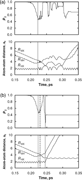 | ||
| Fig. 3 Representative trajectories in the adiabatic representation for the (a) TFS and (b) FSTU methods. The excited state population P2 and internuclear bond distances RAB are shown as functions of time. Downward and upward hops are indicated by solid and dashed vertical lines, respectively. The location of a frustrated hop is shown as a diamond in panel (a). | ||
The FSTU trajectory (Fig. 3(b)) follows the same dynamics as the TFS trajectory up to the frustrated hop. In the FSTU trajectory, the frustrated hop is allowed to hop nonlocally. The FSTU trajectory later hops to the ground state a second time at ∼0.25 ps and finally dissociates to form H+MX products. Note that the “nonlocality” of the hop is only 0.5 fs, and the RHX, RHM, and RMX bond distances change by only 0.02, 0.14, and 0.02 a0, respectively. One may expect these small effects to wash out when averaged over all of the trajectories in the ensemble. We have found, however, that the FSTU method is systematically more accurate than the TFS method.129 Finally, we note that for the 9 realistic, fully-dimensional MXH test cases discussed in Section 4, anywhere from 20% to 95% of trajectories in each test case (with an average of 54%) experience at least one frustrated hopping attempt in the TFS-calculations. Clearly, the treatment of frustrated hops plays an important role in trajectory surface hopping calculations.
For both the TFS and FSTU methods, trajectories experience a discontinuous change in their electronic and nuclear energies when they experience surface hops. These discontinuities may be especially problematic for systems with large energy gaps (which therefore require large energy adjustments at surface hops) or for systems with dense manifolds of electronic states (which may require a large number of small-magnitude surface hops, thus accumulating errors associated with surface hops). The elimination of surface hops (and therefore also of frustrated surface hops) is one motivation for the development of the CSDM method discussed above.
In trajectory surface hopping, a hopping probability is computed at each time step along the classical trajectory. This probability may be sampled in three different ways. In the most widely used sampling scheme (called the “anteater” scheme130), a random number is drawn, and the trajectory hops stochastically according to the hopping probability. The anteater scheme has been successfully applied to a wide variety of systems, but for systems with weakly coupled electronic states, low-probability events may not be efficiently sampled. In the “ants” sampling scheme,130 each trajectory is split into several branches, one of which then propagates on each electronic state. The branches are weighted according to their hopping probabilities. The ants scheme explores nonadiabatic events independent their probabilities, but the large number of resulting branches makes the algorithm computationally prohibitive for most applications. The “army ants” sampling scheme131 has been developed to take advantage of the positive aspects of both the ants and anteater schemes, i.e., it incorporates the stochastic elements of the anteater approach with the weighting scheme of the ants approach. The army ants methods may be efficiently applied to systems with weakly coupled electronic states, and it has been demonstrated131 to be several orders of magnitude more efficient than the ants and anteater schemes for a model system with weakly coupled electronic states. Furthermore it has allowed, for the first time, a demonstration that trajectory surface hopping can agree well with accurate quantum dynamics for weakly coupled systems.131
Now that we have presented the details of four representative semiclassical methods (the first-generation SE and TFS methods and the improved CSDM and FSTU methods), it is instructive to discuss how each method treats coherence effects, which have been discussed in several key articles.13,113,114,132–135 We have restricted our attention to methods that are based on the independent trajectory approximation, in which each trajectory in the ensemble has its own electronic state density matrix ρ that evolves in time according to the unmodified or a modified time-dependent Schrödinger equation. The unmodified Schrödinger equation is solved fully coherently along the trajectory in the SE, TFS, and FSTU methods. Decoherence arises, however, when the electronic state density matrices are averaged over all of the trajectories in the ensemble and the averaging washes out the phases of the off-diagonal elements ρij, although this average is not used in the algorithms. In the SE method, the electronic state density matrices of different trajectories differ due to their different initial coordinates and momenta. In the surface hopping approaches (TFS and FSTU), trajectories may differ for two reasons: differing initial coordinates and differing hopping locations. In this sense, surface hopping methods contain “additional” decoherence. It should be emphasized, however, that this additional decoherence does not affect the dynamics of any single trajectory. The CSDM method contains ensemble averaged decoherence due to the distribution of initial conditions and decoherent state switching locations. The CSDM method also contains an explicit treatment of decoherence (i.e., the effective Schrödinger equation that generates ρ is modified to explicitly include decoherence, as discussed above), and is the most accurate of the methods discussed here.
The CSDM method may be compared with the methods of Rossky and co-workers,13,124,133,135 which also include an explicit treatment of decoherence within the independent-trajectory approach. In these methods, the classical degrees of freedom are treated as a bath, which gives rise to electronic decoherence. A decay time associated with the nuclear motions is derived, and to the extent that we can compare their application to ours (we studied different systems), it is longer than the decay time given by eqn. (16) of the CSDM method. The best formulation for incorporating decoherence into mean-field semiclassical theories remains a area of research that requires further study.
Some authors have modified the surface hopping approach to include a more explicit treatment of coherence. Thachuk et al.134 have demonstrated that fully coherent trajectories can lead to significant errors, and in particular that more accurate methods can be obtained by explicitly destroying decoherence between regions of strong coupling. Parlant and Gislason have developed132 a surface hopping method (which we will call the exact complete passage or ECP method) in which each strong interaction region is treated fully coherently. Surface hops are allowed at local maxima in the coupling, and the hopping probability is determined by integrating the electronic probabilities over the complete passage through each interaction region. Coherence is fully destroyed between strong coupling regions.
Five of the methods discussed above (the SE, CSDM, TFS, FSTU, and ECP methods) are compared in Table 1 to accurate quantum mechanical calculations using the set of 12 test cases described in Section 4. In all of the test cases, an electronically excited atom is scattered off of a diatom, and errors are computed for four probabilities: the probability of nonreactive de-excitation or quenching (PQ), the probability of reactive de-excitation (PR), the total probability of de-excitation (PN), and the fraction of de-excited trajectories that react (FR), and for four “moments”, which are the averages (first moments) of the vibrational and rotational quantum numbers of the reactive and nonreactive de-excited diatomic fragments. In Table 1, we present errors averaged over all 12 test cases; more detailed results can be found elsewhere.74,75,86,113,114Table 1 shows results for the Calaveras County (CC) choice as well as for the adiabatic (A) and diabatic (D) representations.
| Method | Representation | Probabilities | Moments | Averagea |
|---|---|---|---|---|
|
a Average of the Probabilities and Moments columns.
b TFS-
c FSTUgradV
d For YRH cases, the SE method predicts no reactive trajectories over which to average the vibrational and rotational moments. Therefore we cannot compute this entry. If, nevertheless, we average over those cases where we can compute a moment, the mean unsigned relative error is 56%.
e See previous footnote. The average of 69 and 56% is 62%.
f
E
0=0.1 hartree.
|
||||
| TFSb | A | 50 | 29 | 39 |
| D | 211 | 33 | 122 | |
| CC | 48 | 29 | 39 | |
| FSTUc | A | 43 | 29 | 36 |
| D | 107 | 36 | 71 | |
| CC | 40 | 29 | 34 | |
| ECP | A | 73 | 21 | 47 |
| D | 379 | 23 | 201 | |
| CC | 78 | 19 | 49 | |
| SE | all | 69 | d | e |
| CSDMf | A | 23 | 25 | 24 |
| D | 28 | 24 | 26 | |
| CC | 24 | 24 | 24 | |
Results from the trajectory surface hopping methods (TFS, FSTU, and ECP) show strong representation dependence, with average errors for the diabatic representation that are 2–4 times larger than errors for the adiabatic representation. The TFS and FSTU methods differ only in their treatment of frustrated hops, and incorporating nonlocal hopping to alleviate some frustrated surface hops (as in the FSTU method) improves the overall representation independence from a factor of three to a factor of two. As discussed above, the SE self-consistent potential method is formally independent of representation. The decay of mixing in the CSDM method, which is based on the SE approach, builds in some representation dependence, but the errors in the two representations differ only by a factor of 1.1. This improved representation independence is, in fact, one of the motivations for the development of the CSDM method.
Table 1 shows that on average, the CC representation successfully selects the most accurate representation. We note that the CC representation is the diabatic representation for only three of the 12 test cases, and so the CC and adiabatic results are similar. In developing the CC criterion, it was tested against several other proposed criteria using a broader range of test cases, and it was shown to be the most predictive of the several criteria tested.73
Next, we discuss the relative accuracies of the five methods in Table 1 using the CC results. The ECP and TFS methods both perform reasonably well with average errors of 49% and 39%, respectively. The explicit treatment of coherence in the ECP method does not improve the surface hopping approach for the test cases considered here. However, it is possible that a careful treatment of coherence may improve the surface-hopping method, and this remains an area of research. (One reason why the CSDM method outperforms the ECP method is that coherence is not fully destroyed between strong interaction regions, but rather ![[small rho, Greek, tilde]](https://www.rsc.org/images/entities/i_char_e0e4.gif) ij is set equal to ρij. This seems more natural in a self-consistent potential method than in a surface hopping one.) Overall, the FSTU method, which involves only a slight modification of the TFS method, is the most accurate surface hopping method, with an average error of 34%. Along with the improved representation independence of the FSTU method, as discussed above, this makes the FSTU method the clearly preferred surface hopping method.
ij is set equal to ρij. This seems more natural in a self-consistent potential method than in a surface hopping one.) Overall, the FSTU method, which involves only a slight modification of the TFS method, is the most accurate surface hopping method, with an average error of 34%. Along with the improved representation independence of the FSTU method, as discussed above, this makes the FSTU method the clearly preferred surface hopping method.
The SE method, although independent of representation, shows large errors and predicts qualitatively incorrect dynamics. For some of the test cases, the SE method predicts no reactive trajectories, and therefore cannot be used to compute the vibrational and rotational moments associated with the reactive products. The CSDM method improves the accuracy of the self-consistent potential approach and is the best method overall with an average error of only 24% and excellent representation independence. For example, Table 2 shows (for the same methods as Table 1) the probability of reaction and the probability of quenching for Y*+RH (v=0, j)
→ YH+R (PR) or RH (PQ) with initial vibrational quantum number v equal to zero, initial rotational states j, and two coupling strengths Umax12.
+RH collisions at 1.1 eVa
|
U
max12=0.2 eV
j |
U
max12=0.1 eV
j |
||||
|---|---|---|---|---|---|
| Method | Rep.b | P R | P Q | P R | P Q |
| a Same methods as Table 1, compared to accurate quantal calculations b Adiabatic and diabatic representations | |||||
| TFS | A | 0.025 | 0.18 | 0.027 | 0.07 |
| D | 0.161 | 0.40 | 0.066 | 0.17 | |
| FSTU | A | 0.015 | 0.18 | 0.012 | 0.03 |
| D | 0.044 | 0.33 | 0.020 | 0.13 | |
| ECP | A | 0.002 | 0.01 | 0.002 | 0.01 |
| D | 0.359 | 0.55 | 0.146 | 0.36 | |
| SE | A/D | 0.000 | 0.003 | 0.000 | 0.00 |
| CSDM | A | 0.025 | 0.15 | 0.010 | 0.02 |
| D | 0.021 | 0.15 | 0.010 | 0.04 | |
| Accurate | A/D | 0.026 | 0.14 | 0.009 | 0.03 |
6 Summary
We have presented an overview of recent progress on computational non-BO dynamics. These advances include a practical algorithm for computing diabatic energies and couplings called the fourfold way, which may be readily applied to complicated systems. We have discussed the use of the outgoing wave variational principle for computing the accurate quantum dynamics of small reactive scattering systems. The method has been used to develop a set of quantum mechanical results that were used to test approximate methods. Several approximate methods, including methods representative of both the mean-field and surface hopping approaches, have been discussed, and the coherent switching decay of mixing (CSDM) algorithm has been shown to be the most accurate. The CSDM method is the result of several systematic improvements to the self-consistent potential approach. The overall error for this method is ∼25%, which is about the same as or only slightly larger than the errors72 associated with single-surface classical trajectory methods. The CSDM method does not feature quantized vibrations and does not include any treatment of single-surface tunneling, and therefore it is pleasing that using the best available semiclassical methods, the overall errors are dominated by single-surface errors and not the error associated with the nonadiabatic event. The CSDM method has about the same computational cost and only slightly more computational complexity than trajectory surface hopping, and therefore it should be applicable to large and complex systems. It may be used to study the qualitative and semiquantitative features of non-BO systems, just as quasiclassical trajectory methods have been used to elucidate reaction mechanisms and other dynamical features for single-surface reactions.References
- K. Raghavachari and J. B. Anderson, J. Phys. Chem., 1996, 100, 12960 CrossRef CAS.
- See 16 of 17 chapters in Modern Methods for Multidimensional Dynamics Computations in Chemistry, ed. D. L. Thompson, World Scientific, Singapore, 1998 Search PubMed.
- B. O. Roos, Acct. Chem. Res., 1999, 32, 137 CrossRef CAS.
- K. Hirao, Chem. Phys. Lett., 1992, 190, 374 CrossRef CAS.
- H. Nakano, J. Chem. Phys., 1993, 99, 7983 CrossRef CAS.
- K. R. Glaesemann, M. S. Gordon and H. Nakano, Phys. Chem. Chem. Phys., 1999, 1, 967 RSC.
- H. Lischka, R. Shepard, R. M. Pitzer, I. Shavitt, M. Dallos, T. Müller, P. G. Szalay, M. Seth, S. G. Kedziora, S. Yabushita and Z. Zhang, Phys. Chem. Chem. Phys., 2001, 3, 664 RSC.
- K. Kowalski and P. Piecuch, J. Chem. Phys., 2001, 115, 2966 CrossRef CAS.
- J. C. Tully, in Ref. 2, pp. 34–72.
- C. A. Mead and D. G. Truhlar, J. Chem. Phys., 1979, 70, 2284 CrossRef CAS.
- Geometric Phases in Physics, ed. A. Shapere and F. Wilezek, World Scientific, Singapore, 1989 Search PubMed.
- R. B. Griffiths, Consistent Quantum Theory, Cambridge University Press, Cambridge, 2002 Search PubMed.
- O. V. Prezhdo and P. J. Rossky, J. Chem. Phys., 1997, 107, 5863 CrossRef CAS.
- C. P. Sun, X. F. Liu, D. L. Zhou and S. X. Yu, Phys. Rev. A, 2000, 63, 12111 CrossRef.
- M. D. Hack and D. G. Truhlar, J. Chem. Phys., 2001, 114, 9305 CrossRef CAS.
- M. Born and R. Oppenheimer, Ann. Phys., 1927, 84, 457 CAS.
- M. Born, Festschrift Gött. Nachr. Math. Phys., 1951, K1, 1 Search PubMed.
- M. Born and K. Huang, The Dynamical Theory of Crystal Lattices, Oxford University Press, London, 1954 Search PubMed.
- C. A. Mead, in Mathematical Frontiers in Computational Chemical Physics, ed. D. G. Truhlar, Springer-Verlag, New York, 1988, pp. 1–17 Search PubMed.
- J. O. Hirschfelder and W. J. Meath, Adv. Chem. Phys., 1967, 12, 3 CAS.
- J. C. Tully, in Dynamics of Molecular Collisions, Part B, ed. W. H. Miller, Plenum, New York, 1976, pp. 217–267 Search PubMed.
- B. C. Garrett and D. G. Truhlar, Theor. Chem. Adv. Perspect., 1981, 6A, 215 Search PubMed.
- A. D. McLachlan, Mol. Phys., 1961, 4, 417 CAS.
- W. Lichten, Phys. Rev., 1963, 131, 229 CrossRef CAS.
- F. T. Smith, Phys. Rev., 1969, 179, 111 CrossRef.
- T. F. O'Malley, Adv. At. Mol. Phys., 1971, 7, 223 Search PubMed.
- B. C. Garrett, M. J. Redmon, D. G. Truhlar and C. F. Melius, J. Chem. Phys., 1981, 74, 412 CrossRef CAS.
- J. B. Delos, Rev. Mod. Phys., 1981, 53, 287 CrossRef CAS.
- H.-J. Werner and W. Meyer, J. Chem. Phys., 1981, 74, 5802 CrossRef CAS.
- R. Cimiraglia, J. P. Malrieu, M. Persico and F. Spiegelman, J. Phys. B, 1985, 18, 3073 CrossRef CAS.
- T. Pacher, L. S. Cederbaum and H. Köppel, J. Chem. Phys., 1988, 89, 7367 CrossRef CAS.
- T. Pacher, H. Köppel and L. S. Cederbaum, J. Chem. Phys., 1991, 95, 6668 CrossRef CAS.
- V. Sidis, Adv. Chem. Phys., 1992, 82, 73 CAS.
- T. Pacher, L. S. Cederbaum and H. Köppel, Adv. Chem. Phys., 1993, 84, 293 CAS.
- W. Domcke and C. Woywood, Chem. Phys. Lett., 1993, 216, 362 CrossRef CAS.
- G. J. Atchity and K. Ruedenberg, Theor. Chem. Acc., 1997, 97, 47 CrossRef CAS.
- M. Yang and M. H. Alexander, J. Chem. Phys., 1997, 107, 7148 CrossRef CAS.
- V. M. Garcia, M. Reguero, R. Caballol and J. P. Malrieu, Chem. Phys. Lett., 1997, 281, 161 CrossRef CAS.
- E. S. Kryachko and D. R. Yarkony, Int. J. Quantum Chem., 2000, 76, 235 CrossRef CAS.
- T. Takayanagi and Y. Kurosaki, J. Chem. Phys., 2000, 113, 7158 CrossRef CAS.
- M. H. Alexander, D. E. Manolopoulos and H. J. Werner, J. Chem. Phys., 2000, 113, 11084 CrossRef CAS.
- H. Köppel, J. Gronki and S. Mahapatra, J. Chem. Phys., 2001, 115, 2377 CrossRef CAS.
- H. Nakamura and D. G. Truhlar, J. Chem. Phys., 2001, 115, 10353 CrossRef CAS.
- M. Persico, G. Granucci, S. Inglese, T. Laino and A. Toniolo, J. Mol. Struct. (THEOCHEM), 2003, 621, 119 CrossRef CAS.
- C. A. Mead and D. G. Truhlar, J. Chem. Phys., 1982, 77, 6090 CrossRef CAS.
- B. K. Kendrick, C. A. Mead and D. G. Truhlar, Chem. Phys. Lett., 2000, 330, 629 CrossRef CAS.
- B. K. Kendrick, C. A. Mead and D. G. Truhlar, Chem. Phys., 2002, 277, 31 CrossRef CAS.
- A. W. Jasper, B. K. Kendrick, C. A. Mead and D. G. Truhlar, in Modern Trends in Chemical Reaction Dynamics, Part I, ed. K. P. Liu and X. M. Yang, World Scientific, Singapore, 2004, pp. 329–392 Search PubMed.
- D. R. Bates, H. S. W. Massey and A. L. Stewart, Proc. R. Soc. London, Ser. A, 1953, 216, 437.
- B. C. Garrett, D. G. Truhlar and C. F. Melius, in Energy Storage and Redistribution in Molecules, ed. J. Hinze, Plenum, New York, 1983, pp. 375–395 Search PubMed.
- R. J. Buenker and Y. Li, J. Chem. Phys., 2000, 112, 8318 CrossRef CAS.
- A. K. Belyaev, A. Dalgarno and R. McCarroll, J. Chem. Phys., 2002, 116, 5395 CrossRef CAS.
- D. R. Bates and R. McCarroll, Proc. R. Soc. London, Ser. A, 1958, 245, 175.
- J. C. Y. Chen, V. H. Ponce and K. M. Watson, J. Phys. B, 1973, 6, 965 CrossRef CAS.
- H. Nakamura and D. G. Truhlar, J. Chem. Phys., 2002, 117, 5576 CrossRef CAS.
- H. Nakamura and D. G. Truhlar, J. Chem. Phys., 2003, 118, 6816 CrossRef CAS.
- L. Schlessinger, Phys. Rev., 1968, 167, 1411 CrossRef.
- J. Nuttall and H. L. Cohen, Phys. Rev., 1969, 188, 1542 CrossRef.
- Y. Sun, D. J. Kouri, D. G. Truhlar and D. W. Schwenke, Phys. Rev. A, 1990, 41, 4857 CrossRef CAS.
- D. W. Schwenke, S. L. Mielke and D. G. Truhlar, Theor. Chim. Acta, 1991, 79, 241.
- G. J. Tawa, S. L. Mielke, D. G. Truhlar and D. W. Schwenke, in Advances in Molecular Vibrations and Collisional Dynamics, ed. J. M. Bowman, JAI, Greenwich, CT, 1994, Vol. 2B, pp. 45–116 Search PubMed.
- D. W. Schwenke, S. L. Mielke, G. J. Tawa, R. S. Friedman, P. Halvick and D. G. Truhlar, Chem. Phys. Lett., 1993, 203, 565 CrossRef CAS.
- S. L. Mielke, G. J. Tawa, D. G. Truhlar and D. W. Schwenke, J. Am. Chem. Soc., 1993, 115, 6436 CrossRef CAS.
- S. L. Mielke, G. J. Tawa, D. G. Truhlar and D. W. Schwenke, Int. J. Quantum Chem. Symp., 1993, 27, 621 Search PubMed.
- G. J. Tawa, S. L. Mielke, D. G. Truhlar and D. W. Schwenke, J. Chem. Phys., 1994, 100, 5751 CrossRef CAS.
- S. L. Mielke, G. J. Tawa, D. G. Truhlar and D. W. Schwenke, Chem. Phys. Lett., 1995, 234, 57 CrossRef CAS.
- S. L. Mielke, D. G. Truhlar and D. W. Schwenke, J. Phys. Chem., 1995, 99, 16210 CrossRef CAS.
- T. C. Allision, S. L. Mielke, D. W. Schwenke and D. G. Truhlar, J. Chem. Soc. Faraday Trans., 1997, 93, 825 RSC.
- M. S. Topaler, T. C. Allison, D. W. Schwenke and D. G. Truhlar, J. Phys. Chem. A, 1998, 102, 1666 CrossRef CAS.
- M. D. Hack, A. W. Jasper, Y. L. Volobuev, D. W. Schwenke and D. G. Truhlar, J. Phys. Chem. A, 1999, 103, 6309 CrossRef CAS.
- M. S. Topaler, M. D. Hack, T. C. Allison, Y.-P. Liu, S. L. Mielke, D. W. Schwenke and D. G. Truhlar, J. Chem. Phys., 1997, 106, 8699 CrossRef CAS.
- M. S. Topaler, T. C. Allison, D. W. Schwenke and D. G. Truhlar, J. Chem. Phys., 1998, 109, 3321 CrossRef CAS; M. S. Topaler, T. C. Allison, D. W. Schwenke and D. G. Truhlar, J. Chem. Phys., 1999, 110, 687 CrossRef CAS , erratum M. S. Topaler, T. C. Allison, D. W. Schwenke and D. G. Truhlar, J. Chem. Phys., 2000, 113, 3928 Search PubMed , erratum.
- M. D. Hack, A. W. Jasper, Y. L. Volobuev, D. W. Schwenke and D. G. Truhlar, J. Phys. Chem. A, 2000, 104, 217 CrossRef CAS.
- Y. L. Volobuev, M. D. Hack, M. S. Topaler and D. G. Truhlar, J. Chem. Phys., 2000, 112, 9716 CrossRef CAS.
- A. W. Jasper, M. D. Hack and D. G. Truhlar, J. Chem. Phys., 2001, 115, 1804 CrossRef CAS.
- Y. L. Volobuev, M. D. Hack and D. G. Truhlar, J. Phys. Chem. A, 1999, 103, 6225 CrossRef CAS.
- L. D. Landau, Phys. Z. Sowjetunion, 1932, 2, 46 Search PubMed.
- C. Zener, Proc. R. Soc. London, Ser. A, 1932, 137, 696 CrossRef.
- E. Teller, J. Chem. Phys., 1932, 41, 109.
- N. Rosen and C. Zener, Phys. Rev., 1932, 18, 502 CrossRef CAS.
- Yu. N. Demkov, J. Exp. Theor. Phys., 1963, 45, 195 ( Sov. Phys. JETP , 1963 , 18 , 138 ) CAS.
- Yu. N. Demkov, Dokl. Akad. Nauk SSSR, 1966, 166, 1076 Search PubMed; Yu. N. Demkov, Sov. Phys. Dokl., 1966, 11, 138 Search PubMed.
- M. S. Child, in Atom-Molecule Collision Theory, ed. R. B. Bernstein, Plenum, New York, 1979, pp. 427–465 Search PubMed.
- S. Chapman, Adv. Chem. Phys., 1992, 82, 423.
- J. C. Tully, Faraday Discuss., 1998, 110, 407 RSC.
- M. D. Hack and D. G. Truhlar, J. Phys. Chem. A, 2000, 104, 7917 CrossRef CAS.
- D. G. Truhlar and J. T. Muckerman, in Atom–Molecule Collision Theory, ed. R. B. Bernstein, Plenum, New York, 1979, pp. 505–566 Search PubMed.
- R. B. Gerber, V. Buch and M. A. Ratner, J. Chem. Phys., 1982, 77, 3022 CrossRef CAS.
- V. Buch, R. B. Gerber and M. A. Ratner, Chem. Phys. Lett., 1983, 101, 44 CrossRef CAS.
- R. Alimi, R. B. Gerber, A. D. Hammerich, R. Kosloff and M. A. Ratner, J. Chem. Phys., 1990, 93, 6484 CrossRef CAS.
- C. C. Martens and J.-Y. Fang, J. Chem. Phys., 1997, 106, 4918 CrossRef CAS.
- J. C. Burant and J. C. Tully, J. Chem. Phys., 2000, 112, 6097 CrossRef CAS.
- S. Nielsen, R. Kapral and G. Ciccotti, J. Chem. Phys., 2000, 112, 6543 CrossRef CAS.
- A. Donoso, D. Kohen and C. C. Martens, J. Chem. Phys., 2000, 112, 7345 CrossRef CAS.
- M. Sauter, U. Manthe and G. Stock, J. Chem. Phys., 2001, 114, 2001 CrossRef.
- A. Donoso and C. C. Martens, Int. J. Quantum Chem., 2002, 90, 1348 CrossRef CAS.
- C.-C. Wan and J. Schofield, J. Chem. Phys., 2002, 116, 494 CrossRef CAS.
- K. Ando and M. Santer, J. Chem. Phys., 2003, 118, 10399 CrossRef CAS.
- A. Sergi, D. MacKernan, G. Cicotti and R. Kapral, Theor. Chem. Acc., 2003, 110, 49 Search PubMed.
- E. J. Heller, J. Chem. Phys., 1975, 62, 1544 CrossRef CAS.
- E. J. Heller, J. Chem. Phys., 1981, 75, 2923 CrossRef CAS.
- M. D. Hack, A. M. Wensmann, D. G. Truhlar, M. Ben-Nun and T. J. Martinez, J. Chem. Phys., 2001, 115, 1172 CrossRef CAS.
- T. J. Martinez, M. Ben-Nun and R. D. Levine, J. Phys. Chem., 1996, 100, 7884 CrossRef CAS.
- T. J. Martinez, M. Ben-Nun and R. D. Levine, J. Phys. Chem., 1997, 101, 6839 Search PubMed.
- H.-D. Meyer and G. A. Worth, Theor. Chem. Acc., 2003, 109, 251 Search PubMed.
- I. Burghardt, M. Nest and G. A. Worth, J. Chem. Phys., 2003, 119, 5364 CrossRef CAS.
- J. C. Tully, J. Chem. Phys., 1990, 93, 1061 CrossRef CAS.
- H. Wang, M. Thoss and W. H. Miller, J. Chem. Phys., 2001, 115, 2979 CrossRef CAS.
- A. García-Vela, R. B. Gerber and D. G. Imre, J. Chem. Phys., 1992, 97, 7242 CrossRef CAS.
- D. A. Micha, J. Chem. Phys., 1983, 78, 7138 CrossRef CAS.
- M. Amarouche, F. X. Gadea and J. Durup, Chem. Phys., 1989, 130, 145 CrossRef CAS.
- A. Bohm, Quantum Mechanics: Foundations and Applications, Springer-Verlag, New York, 3rd edn., 1993, pp. 63ff Search PubMed.
- C. Zhu, S. Nangia, A. W. Jasper and D. G. Truhlar, in preparation.
- C. Zhu, A. W. Jasper and D. G. Truhlar, J. Chem. Phys., 2004, 120, 5543 CrossRef CAS.
- W. H. Zurek, Phys. Rev. D, 1981, 24, 1516 CrossRef.
- J. P. Paz and W. H. Zurek, Phys. Rev. Lett., 1999, 26, 5181 CrossRef.
- P. Ehrenfest, Z. Phys., 1927, 45, 455.
- L. I. Schiff, Quantum Mechanics, McGraw-Hill, New York, 3rd edn., 1968, pp 28–30 Search PubMed.
- H.-D. Meyer and W. H. Miller, J. Chem. Phys., 1980, 72, 2272 CrossRef CAS.
- M. F. Herman, J. Chem. Phys., 1984, 81, 754 CrossRef CAS.
- D. F. Coker and L. Xiao, J. Chem. Phys., 1995, 102, 496 CrossRef CAS.
- G. A. Fiete and E. J. Heller, Phys. Rev. A, 2003, 68, 22112 CrossRef.
- R. S. Berry, S. A. Rice and J. Ross, Physical Chemistry, Oxford University Press, New York, 2nd edn., 2000, p. 199 Search PubMed.
- L. Turi and P. J. Rossky, J. Chem. Phys., 2004, 120, 3688 CrossRef CAS.
- S. Hammes-Schiffer and J. C. Tully, J. Chem. Phys., 1994, 101, 4657 CrossRef CAS.
- W. H. Miller and T. F. George, J. Chem. Phys., 1972, 56, 5637 CrossRef CAS.
- U. Müller and G. Stock, J. Chem. Phys., 1997, 107, 6230 CrossRef CAS.
- A. W. Jasper, S. N. Stechmann and D. G. Truhlar, J. Chem. Phys., 2002, 116, 5424 CrossRef CAS; A. W. Jasper, S. N. Stechmann and D. G. Truhlar, J. Chem. Phys., 2002, 117, 10427 CrossRef CAS , erratum.
- A. W. Jasper and D. G. Truhlar, Chem. Phys. Lett., 2003, 369, 60 CrossRef CAS.
- R. K. Preston and J. C. Tully, J. Chem. Phys., 1971, 54, 4297 CrossRef CAS.
- S. Nangia, A. W. Jasper, T. F. Miller III and D. G. Truhlar, J. Chem. Phys., 2004, 120, 3586 CrossRef CAS.
- G. Parlant and E. A. Gislason, J. Chem. Phys., 1989, 91, 4416 CrossRef CAS.
- B. J. Schwarz, E. R. Bittner, O. V. Prezhdo and P. J. Rossky, J. Chem. Phys., 1996, 104, 5942 CrossRef CAS.
- M. Thachuk, M. Y. Ivanov and D. M. Wardlaw, J. Chem. Phys., 1998, 109, 5747 CrossRef CAS.
- K. F. Wong and P. J. Rossky, J. Chem. Phys., 2002, 116, 8429 CrossRef CAS.
| This journal is © The Royal Society of Chemistry 2004 |