Changes in biologically active ultraviolet radiation reaching the Earth's surface

Abstract

Since publication of the 1998 UNEP Assessment, there has been continued rapid expansion of the literature on UV-B radiation. Many measurements have demonstrated the inverse relationship between column ozone amount and UV radiation, and in a few cases long-term increases due to ozone decreases have been identified. The quantity, quality and availability of ground-based UV measurements relevant to assessing the environmental impacts of ozone changes continue to improve. Recent studies have contributed to delineating regional and temporal differences due to aerosols, clouds, and ozone. Improvements in radiative transfer modelling capability now enable more accurate characterization of clouds, snow-cover, and topographical effects.

A standardized scale for reporting UV to the public has gained wide acceptance. There has been increased use of satellite data to estimate geographic variability and trends in UV. Progress has been made in assessing the utility of satellite retrievals of UV radiation by comparison with measurements at the Earth's surface. Global climatologies of UV radiation are now available on the Internet.

Anthropogenic aerosols play a more important role in attenuating UV irradiances than has been assumed previously, and this will have implications for the accuracy of UV retrievals from satellite data. Progress has been made inferring historical levels of UV radiation using measurements of ozone (from satellites or from ground-based networks) in conjunction with measurements of total solar radiation obtained from extensive meteorological networks.

We cannot yet be sure whether global ozone has reached a minimum. Atmospheric chlorine concentrations are beginning to decrease. However, bromine concentrations are still increasing. While these halogen concentrations remain high, the ozone layer remains vulnerable to further depletion from events such as volcanic eruptions that inject material into the stratosphere. Interactions between global warming and ozone depletion could delay ozone recovery by several years, and this topic remains an area of intense research interest.

Future changes in greenhouse gases will affect the future evolution of ozone through chemical, radiative, and dynamic processes. In this highly coupled system, an evaluation of the relative importance of these processes is difficult; studies are ongoing. A reliable assessment of these effects on total column ozone is limited by uncertainties in lower stratospheric response to these changes.

At several sites, changes in UV differ from those expected from ozone changes alone, possibly as a result of long-term changes in aerosols, snow cover, or clouds. This indicates a possible interaction between climate change and UV radiation. Cloud reflectance measured by satellite has shown a long-term increase at some locations, especially in the Antarctic region, but also in Central Europe, which would tend to reduce the UV radiation.

Even with the expected decreases in atmospheric chlorine, it will be several years before the beginning of an ozone recovery can be unambiguously identified at individual locations. Because UV-B is more variable than ozone, any identification of its recovery would be further delayed.

Ozone changes

Since the previous assessment in 1998,^3,4 there have been improvements in assimilating global ozone data from several sources, resulting in a more cohesive picture of how ozone has changed since the early 1990s when one of the few satellite sensors measuring long-term changes in global ozone failed (NASA's Total Ozone Mapping Spectrometer, TOMS, on the Nimbus 7 satellite). These re-analyses⁶ show that the pattern of change since 1994 has been essentially a continuation of that before the eruption of Mt Pinatubo. Ozone changes continue to be insignificant in the tropics. At mid-latitudes, ozone depletion appears to be levelling off. In the Arctic, ozone has been highly variable, and in Antarctica it has remained similar to that during the 1990s. Because the ozone changes have not been monotonic, and with the expected future recovery, a linear trend analysis of ozone change is no longer appropriate.

The Antarctic ozone hole has continued to appear each spring. In 2000 its area, defined as the region where ozone is less than 220 DU, reached a record maximum size of 29 million km² (about twice the size of the Antarctic continental land mass), with a maximum depleted mass of 57 megatons (Mt) but it then rapidly dissipated much earlier than usual. During the spring of 2001, the area and depleted mass were 25 million km² and 54 Mt, respectively (slightly less than the record values of the previous year). As in recent years, the hole persisted well into November, leading to potentially larger UV radiation effects.^7–9 The Antarctic ozone minimum in recent years has been about 90–100 DU, which is less than 40% of the minima typical for Antarctica in the late 1970s, before the ozone hole first developed. The minimum recorded ozone column occurred in 1993 when other factors (e.g., aerosols from the volcanic eruption of Mt Pinatubo) contributed to a particularly severe depletion of ozone.

In the Arctic, ozone depletion remains less severe than in the Antarctic, with minimum ozone amounts typically in the range 200–250 DU. The extent of ozone depletion in the Arctic is more dependent on year-to-year variability in wind patterns. Depletions are more severe when the Arctic stratosphere is cold in the winter/spring. In the cold spring of 2000, the accumulated loss of ozone near 20 km altitude, where ozone depletion was most severe, reached roughly 20% by mid-February. This is a moderate chemical loss compared to Arctic winters during the last decade, when ozone losses as high as 70% have been observed at some altitudes.

Outside the Polar Regions, ozone losses are less severe. Relative to 1980, the 1997–2000 losses in total ozone are about 6% at southern mid-latitudes on a year-round basis. At northern mid-latitudes the ozone losses are about 4% in winter/spring, and 2% in summer/autumn. In the tropics, there have been no significant changes in column ozone. The annually averaged global ozone loss is approximately 3%.⁶ These changes in ozone are broadly consistent with the changes predicted by atmospheric models.

There remain unresolved differences between satellite and ground based measurements of ozone. For example, the TOMS instruments currently overestimate ozone at high latitudes, especially in the Southern hemisphere summer.¹⁰

At any single observation site, the year-to-year variability in ozone hinders our ability to detect long-term trends in ozone. Similarly, it has been demonstrated that any detection of future ozone recovery (and of consequent UV recovery) will not be possible for several years or even decades. Mid-latitudes of the Southern hemisphere appear to offer the earliest possibility of detection of recovery.¹¹ To detect global trends in ozone, it is necessary to use large spatial averaging such as from the global network of ground-based spectrometers, or from satellite data.

Polar ozone-depleting processes are now better understood, but uncertainties remain about ozone depletion processes at mid-latitudes. These processes could influence how global warming affects future ozone depletion. The importance of long-term changes in dynamics, possibly forced by changes in climate, in driving ozone change is now better appreciated.

Factors affecting UV radiation received at the Earth's surface

Variability in ozone is not the dominant factor affecting UV-B radiation received at the surface. The dominant factor is the angle of the Sun's rays through the atmosphere. This angle is often given in terms of the solar zenith angle (SZA – which is the angle between the vertical and the center of the solar disc). When the SZA is small, the light path through the atmosphere is small, so absorption is minimised. For this reason the maximum UV-B irradiances occur in the tropics at times when the Sun is directly overhead. In these regions ozone amounts are also relatively low. At mid- and high latitudes the UV-B irradiances in winter are much smaller than in the summer. Consequently even with extremely low ozone amounts, as under the springtime Antarctic ozone hole, UV-B irradiances only rarely reach the levels that are normal in the tropics.^12,13 Variability in cloud cover is the second major factor influencing surface UV-B. The importance of these factors is illustrated clearly by results from a network of erythemal UV sensors that cover a wide range of latitudes in Argentina,¹⁴ and from global analyses based on satellite data (e.g., Fig. 4).

The effect on surface UV of ozone depletion depends on the wavelength range of interest, shorter wavelengths in the UV-B region being more sensitive. For many processes of environmental interest, a reduction in ozone of 1% leads to an increase in damaging radiation of 0.2 to 2%, depending on the wavelength-dependence of the sensitivity, as described by the so-called Radiation Amplification Factor (or RAF).¹⁵

Other factors affecting surface UV radiation include seasonal variations in Sun–Earth separation, extinctions by aerosols, altitude, and surface reflectivity (albedo). Several of these are discussed later.

UV information to the public

There have been significant improvements in the delivery of UV information to the public. An internationally standardized UV Index has been defined,¹⁶ by which information on UV intensities is disseminated to the public (see box).

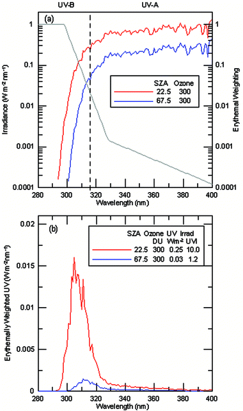
UV Index

The internationally agreed UV Index scale is defined in terms of the erythemally weighted UV irradiance (i.e. “skin-reddening”, or “sunburning” irradiance). The erythemal weighting function, which is applied to the spectrum, involves an arbitrary normalization to unity at wavelengths shorter than 298 nm, so erythemally weighted UV is not strictly defined in terms of an SI unit. Furthermore, when UV information was first provided to the public, another normalization (a multiplication by 40 m² W⁻¹) was applied to provide a number, called the UV Index. With this normalization, the maximum UV Index in Canada (where the unit was first used) is about 10 for normal ozone conditions.

UV Index = 40∫ I(λ) w(λ) dλ,

where:

λ is the wavelength in nm,

I(λ) is the irradiance in W m⁻² nm⁻¹ , and w(λ) is the erythemal weighting function which is defined as:

w(λ) = 1.0 for 250 <λ≤ 298 nm

w(λ) = 10^{0.094(298 − λ)} for 298 < λ ≤ 328 nm

w(λ) = 10^{0.015(139 − λ)} for 328 < λ ≤ 400 nm

w(λ) = 0.0 for λ > 400 nm

The upper panel shows the spectral UV irradiance for two sun angles; with an ozone column amount of 300 DU. The erythemal weighting function is shown on the right axis. The lower panel shows the corresponding spectra of erythemally weighted UV. The UV Index is the integral under these curves multiplied by 40 m² W⁻¹.

Although there are uncertainties about the biological applicability of this erythemal action spectrum, its advantage is that it is mathematically defined and therefore its detailed shape is unambiguous. This is important in the UV region where the steeply sloping spectrum spans several orders of magnitude. Although the UV Index was developed to represent damage to human skin, it may be applied to other processes, since many biological UV effects have similar action spectra. Since the UV Index is based on the erythemal action spectrum, its sensitivity to ozone change is the same as for erythema. For small reductions in ozone, the change in UV Index can be estimated by the radiative amplification factor, where for each 1% reduction in ozone the UV Index increases by approximately 1.1% (i.e., the RAF for erythema is 1.1, as detailed elsewhere).¹⁵ However, this formulation underestimates the change for large changes in ozone. In that case the power law formulation of the sensitivity is required, as noted previously.¹⁵

In reality, the UV Index is an open-ended scale. In the tropics, at unpolluted mid-latitudes in the Southern hemisphere, and at high altitudes it often exceeds a value of 12.^14,17,18 Outside the protection of the Earth's atmosphere the UV Index is ∼300 (depending on the lower wavelength limit of the integration). To calculate the UV Index, estimates of ozone are required as inputs to a radiative transfer model. Atmospheric dynamical forecasts are sometimes used to predict how the ozone will change between the measurement time and the prediction time. Corrections to account for reductions by clouds are applied by some reporting agencies, but not all. The use of satellite derived ozone and cloud fields (see later) has improved the timely delivery of UV Index information to the public.

Measurements of UV at the surface

Ground based measurements

There has been a significant improvement in the geographical coverage of instruments to measure UV,¹⁴ and in their quality control and quality assurance. The UV data are now more readily available through international data archives such as the World Ozone and UV Data Centre (WOUDC, see http://www.msc-smc.ec.gc.ca/woudc/) in Canada, and the European Database created through EU research projects (EDUCE, see http://www.muk.uni-hannover.de/EDUCE). In combination with radiative transfer models, these measurements have confirmed the expected inverse correlation between ozone and UV-B. In addition, the effects of other variables are now better understood.⁶

Data availability, quality control and quality assurance. Recent international intercomparisons between spectroradiometers have demonstrated agreement within limits comparable to the uncertainties in maintaining irradiance standards via lamp transfer standards.¹⁹ Progress has been made using Langley analyses of spectra to derive a calibration based on solar extraterrestrial spectra.^20,21 This procedure avoids the need for radiometric calibrations via quartz halogen lamps (such as 1000 W FEL lamps calibrated by the National Institute of Standards and Technology (NIST)), which are difficult to maintain and use. However, it has not yet been successfully applied at the shorter wavelengths in the UV-B region at many sites.

Results from more recently established UV monitoring networks (e.g., in Europe and South America) are contributing to the characterisation of geographic differences.^14,22–27

Altitude effects. The effect of altitude on UV irradiance has been better quantified. In practice the altitude effect depends on differences in surface albedo and boundary layer extinctions by aerosols and tropospheric ozone, so it cannot be represented by a single number. Even when these effects can be ignored, it has been found that the altitude effect is a strong function of the solar zenith angle and wavelength. For erythemally weighted UV, irradiances increase by approximately 5 to 7 percent per kilometer (for the same overhead ozone column), with the greatest increase occurring at SZA ∼ 60–70°. To correctly model the effect at Mauna Loa Observatory, it was necessary to consider the effects of sky irradiance scattered from below the observatory.¹⁸ Recent measurements in Europe, which included aerosol and albedo effects, showed much larger and more variable increases.²⁸ Aircraft measurements in the free troposphere over Greece have revealed larger altitude gradients than at pristine sites.²⁹

Surface albedo effects. The presence of snow cover in the surrounding area can increase UV irradiances appreciably,^30,31 even when the snow is several kilometers away from the observing site.^32,33 Furthermore, increases in effective surface albedo due to reflectances from air below the observing site can also be important.¹⁸ An implication of these findings is that three-dimensional radiative transfer models are needed to accurately model UV irradiances in mountainous regions. Codes suitable for this purpose are being developed and are becoming available.^34–37

Cloud effects. Cloud effects are important. The mean attenuation of UV-B by clouds is typically in the range 15–30%. There have been improvements in the measurement of clouds from automated imagers at the Earth's surface. Progress has been made relating these cloud images to satellite-derived cloud patterns and to the UV radiation received at the Earth's surface.³⁸ There is evidence for long-term changes in cloud in some regions, as discussed later.³⁹

Aerosol effects. Aerosols can have a marked effect on the UV-B radiation received at the surface. In some locations aerosols can scatter more than 50% of UV-B radiation out of the direct beam.⁴⁰ In Mexico City, poor air quality has been shown to be responsible for reductions of ∼20% in erythemal UV in the city centre compared with the suburbs.⁴¹ The optical properties of aerosols, as measured in the Eastern USA, have been shown to have a strong impact on UV-B at the surface. In extreme cases during the summertime, aerosol extinctions can result in reduction of the UV Index by up to 5 units, representing reductions of approximately 50%. More typically however, the deduced reductions are less than 20%.⁴²

Recent work suggests that anthropogenic aerosols (e.g., from urban pollution) that absorb in the UV-B region may play a more important role in attenuating UV-B irradiances than has been assumed previously.⁴³ Measurements in the Los Angeles region have shown that near-surface absorption is much larger in the UV-B than in the visible region. Direct measurements of aerosol absorptions and single scattering albedos of aerosols will be helpful in resolving the importance of aerosols.

Comparisons between satellite-derived UV and measurements from four cross-calibrated ground-based spectrometers have revealed inconsistencies in satellite-derived UV. The discrepancy is probably related to the inability of the satellite sensors to correct for extinctions in the lowermost region of the atmosphere (i.e., in the “boundary layer”). Only at the pristine site was there good agreement within the experimental errors. At more polluted sites, the satellite-derived UV estimations were too large.⁴⁴

These findings, and the much larger altitude gradients of UV reported in polluted regions, suggest that boundary layer extinctions from man made pollutants may be more important attenuators of UV than has previously been recognised.

As discussed later, the effects of urban pollution may extend over wide geographical areas. Recurring episodes of biomass burning, which contribute to increased particulates and altered gas composition, can lead to reduced UV-B at the surface and in the troposphere,^23,45,46 but with attendant increases in other health risk factors.

Actinic fluxes. For many biological and photochemical processes, including atmospheric photochemistry, irradiances falling on a horizontal surface are not the most relevant quantity. It has been shown that the irradiance on surfaces of different orientations can differ markedly from that on a horizontal surface. In particular for surfaces directed towards the sun, or for vertical surface facing the sun at large SZA, irradiances can be significantly greater than on a horizontal surface.^47,48 For many applications, the target is insensitive to the direction of incoming radiation, and for those cases actinic flux (sometimes called scalar flux, or scalar irradiance, or fluence rate) rather than cosine-weighted irradiance may be more appropriate. However, such measurements have not been generally available until quite recently.^49,50 Progress has been made in converting irradiance to actinic flux and this work offers the prospect of deriving historical changes from the more extensive database of irradiance measurements.^51–53

Long-term changes in UV measured from the ground

The complicated spatial and temporal distributions of the variables that affect ultraviolet radiation at the surface (for example, clouds, airborne fine particles, snow cover, sea ice cover, and total ozone) continue to limit the ability to describe surface ultraviolet radiation on the global scale, whether through measurements or model-based approaches. The spectral surface ultraviolet data records, which started in the early 1990s, are still too short and too variable to permit the calculation of statistically significant long-term (i.e., multi-decadal) trends.

Many studies have demonstrated the inverse correlation between ozone and UV. However, the detection of long-term trends in UV is even more problematic than the detection of ozone trends because in addition to its dependence on ozone, UV radiation at the surface is sensitive to clouds, aerosols, and surface albedo, all of which can exhibit large variability.

In Moscow, changes in atmospheric opacity from clouds and/or aerosols were probably responsible for a reported gradual decrease in UV from the 1960s to the mid 1980s, followed by an increase back to 1960s levels by the late 1990s.⁵⁴

One of the longest time series of UV-B data available is that from Robertson–Berger (RB) meter measurements from Belsk, Poland. An analysis of data over the period 1976 to 1997 in all weather conditions shows an increase in sunburning UV of 6.1 ± 2.9 percent per decade, which is attributed mainly to ozone change.⁵⁵

An increase in peak UV in response to decreasing ozone has been detected in New Zealand, as shown in Fig. 1.^5,56 However, the trend has not continued in the last two summers. In these two summers, ozone amounts at this site have been slightly higher than in the summer of 1998–99. Furthermore, both years were rather cloudy over the summer period that is most critical for this analysis. This shows that year-to-year variability in cloud cover can have a significant effect even for peak irradiances.

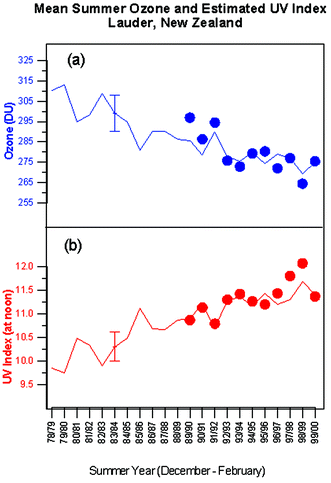Fig. 1 (a) Mean ozone (Dobson Units, 1 DU = 2.69 × 10¹⁶ molecule cm⁻²), and (b) estimated UV Index at Lauder, New Zealand for the summers of 1978–79 through 1999–2000. Summer is defined as the period from December through February. The solid line in (a) shows the changes in summertime ozone that have occurred since the 1970s. The solid line in (b) shows the deduced changes in clear-sky UV expected from these changes in ozone. The dots (from 1989–90 on) show measured values of ozone and the summertime peak UV Index, both derived from the UV spectroradiometer.⁵

A 10-year record of UV measurements in Thessaloniki, Greece indicates significant increases in erythemal UV irradiance and in irradiance at the lower UV-B wavelengths (e.g., 305 nm) which is partly caused by ozone decreases and partly by the cleaning of the atmosphere by air-pollution abatement measures.⁵⁷ Other medium term dynamical effects, such as the Quasi Biennial Oscillation (QBO) in atmospheric wind patterns with a period of about 2 years, are also significant.^58,59 Long term changes and year-to-year variability have also been observed in Antarctica.⁶⁰

Broadband UV-B monitors are generally less suitable for trend detection, since their calibration is less direct and the quality assurance of long-term calibrations is more problematic. Recently it has been shown that the spectral response functions of some broad band instruments in common usage for measuring sunburning UV are sensitive to relative humidity.⁶¹ The largest sensitivity is in the UV-A region, where instrument response varies, sometimes reversibly, over time scales of hours.¹⁰ The implication of this finding is that in instruments where desiccant is not replenished regularly, readings may have large time-dependent errors between calibrations.

Inferring UV changes from indirect methods

A limitation on trend detection is the relatively short time period for which suitable UV measurements are available. However, methods have been developed to estimate the effects of clouds on UV from total solar radiation measurements (i.e., pyranometer data) and so to derive long-term estimates of UV using historical pyranometer data in conjunction with ozone measurements. Initially these used ozone data from satellite, so enabling estimation of long-term changes from 1978 to the present.

A recent study of this kind in Canada used a longer time series of ozone data from a network of ground-based instruments to derive trends from the mid-1960s at Toronto, Churchill and Edmonton.¹ Trends in UV for individual wavelengths and weighted spectral intervals have been determined for the period from 1965 to 1997 (see Fig. 2).

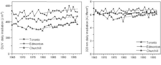Fig. 2 Mean summer (May–August) daily UV irradiation for Toronto, Edmonton, and Churchill, Canada.¹ Left Panel: damaging UV radiation (DUV), as defined by the American Conference of Governmental Industrial Hygienists – National Institute of Occupational Safety and Health (defined in 1). Right panel: 320 nm, which is insensitive to ozone change.

Trends in the daily total values and noontime values are essentially the same, and trends at wavelengths of 310 nm or less and for the erythemally weighted UV are all statistically significant at the 2-sigma level. In addition to the estimation of past hour-by-hour UV irradiance, the data can be used to quantify and distinguish between trends in UV that are caused by factors other than long-term changes in total ozone. Churchill had statistically significant trends at all wavelengths, including those with insignificant ozone absorption. The positive trends at these wavelengths are due to the combined effect of an increase of days with snow cover and a decrease in hours of cloudiness that occurred at Churchill over the period (1979–1997). Although the increases in damaging UV were rather modest, there was a more marked increase in the occurrence of extreme events such as the number of hours that the UV Index exceeded a threshold value (see Fig. 3).

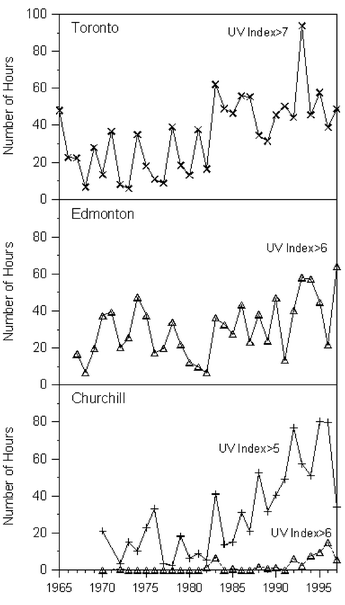Fig. 3 Number of hours when the hourly mean UV index exceeded 7 at Toronto, 6 at Edmonton, 5 and 6 at Churchill.¹

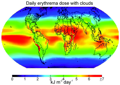Fig. 4 Global climatology (1979–1992) of mean daily erythemal UV dose (from the NCAR web site http://www.acd.ucar.edu/TUV/).

Statistical methods, using pyranometer data in conjunction with ozone measurements, have also been applied in other geographical regions to deduce long-term increases in surface UV in several parts of Europe^62,63 as well as in the Arctic and Antarctic.⁶⁰ These increases are in agreement with those expected from changes in satellite-measured ozone. At the South Pole, the deduced springtime increases from 1979 to 1996 in 300 nm radiation are ∼300% during spring, while at Barrow, Alaska corresponding increases of ∼100% have been inferred. Increases in biologically weighted UV would, however, be much less than those at 300 nm.

By selecting for clear sky data only, large statistically significant increases have been reported over a 30-year period in Bavaria. This was achieved by deriving statistical relationships between UV and ozone and using diffuse/direct ratios from pyranometers to characterize aerosol extinction classes.⁶⁴ Significant increases at the longer wavelengths indicate that not all of the change is due to ozone depletion.

Estimations of UV from satellite observations

Satellite methods provide the greatest potential for assessing geographical variations in UV radiation. Products that are currently available include UV dose and UV irradiances. Both are available with or without the effects of clouds.

Increasingly these data are becoming freely available through the Internet, and are produced in near real time. In some cases models are used to predict ozone and cloud patterns for several days into the future (e.g., by NOAA, National Weather Service see web site http://www.cpc.ncep.noaa.gov/products/stratosphere/). These UV forecasts are then provided to the public through the media.

From these data, global climatologies of UV, such as that shown in Fig. 1, can be derived. The dominant feature here is the strong latitudinal gradient, with highest doses of UV occurring in the tropics. As noted below, however, questions remain about the absolute accuracy of these products.

Methods have recently been developed to generate regional-scale maps of surface UV radiation (Fig. 4), including cloud effects, using satellite data of higher spatial and temporal resolution, along with ancillary geophysical data.⁶⁵

Measurements from satellite also provide the potential for deriving accurate trends in UV, since only a single sensor needs to be characterized for the lifetime of that satellite instrument, and since the global coverage offers the potential to average out variability caused by changing cloud patterns. However, the insensitivity to changes in tropospheric extinctions currently limits the ability of satellite data products to be used in trend studies.

In one study, satellite-derived estimates of erythemal UV incident in Australia showed larger increases in the tropics than at mid-latitudes over the period 1979–1992, due to the combined influence of changes in ozone and clouds.⁶⁶ Another study of satellite-derived erythemal UV trends in the Northern hemisphere (1979–91) showed marked regional differences. At latitudes 30–40°N, trends were larger over oceans, while at 40–60°N they were larger over continental areas. The largest trends were seen over northeast Asia where they exceeded 10% per decade for May–August.⁶⁷

A study using satellite data has demonstrated that long-term changes in cloud cover have occurred in some regions.⁶⁸ For example, according to this analysis, cloud cover has increased in parts of Antarctica, and this would have suppressed some of the increase in UV expected from ozone loss over the same period.^6,68,69

Comparisons between UV measured at the ground and from satellite

The determination of surface UV from satellite observations is essentially a model calculation. Key atmospheric variables such as ozone and cloud reflectance, which are available from the satellite-borne sensors, are used as input parameters to the model calculation. In the case of satellite instruments that measure backscattered ultraviolet radiation, one of the difficulties is the insensitivity to radiation that penetrates deep into the troposphere. Consequently, it is necessary to make assumptions about the radiative transfer in the boundary layer. In this region, local differences in ozone, clouds, and aerosols can be important. One example of these difficulties is that satellite-derived ozone amounts can be overestimated in regions where the tropospheric ozone component is lower than assumed in the retrieval algorithm. This is most likely the cause of the overestimation¹⁰ of satellite-derived ozone in the southern hemisphere summer. This ozone error would tend to translate to lower than expected estimates of surface UV. A second issue relates to the assumption that the complement of the reflected component is transmitted to the surface. With complex broken clouds, three-dimensional effects also become important, particularly in analyses at high spatial and temporal resolution. A further limitation of polar orbiting satellites is that there is generally only one overpass per day, whereas studies with geo-stationary satellite data have demonstrated that several cloud images over the midday period are desirable for determining UV dose.⁶⁵ Finally, satellite sensors are not yet capable of measuring extinctions from the ubiquitous non-absorbing aerosols in the boundary layer. As discussed above, these aerosol extinctions can have a marked effect on UV at the surface.

There have been several intercomparisons between UV measured at the ground and satellite-derived UV.^70–72 Difficulties in these studies include (1) uncertainties in the ground-based measurements, and (2) the assumption that the specific ground location is representative of the entire satellite pixel, which typically covers a much larger geographical area.

A comprehensive study compared UV measured over several years at four mid-latitude sites using cross-calibrated, state-of-the-art spectrometer systems.⁴⁴ The conclusion from that study was that although broad patterns of UV can be derived from satellite data there could be large systematic differences (see Fig. 5). In some regions, UV measured at the ground is ∼40% less than that derived from satellite data. One implication from these tropospheric aerosol and ozone effects is that differences in satellite-derived UV between polluted and unpolluted locations (e.g., mid northern latitudes versus mid southern latitudes) will be suppressed.

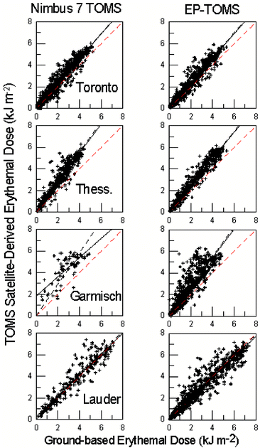Fig. 5 Scatter plots of TOMS-derived erythemal UV as a function of UV measured at four sites: Toronto, Canada (43.4°N); Thessaloniki, Greece (40.5°N); Garmisch-Partenkirchen, Germany (47.5°N), and Lauder, New Zealand (45.0°S). Note the more intense UV at the Southern hemisphere site. The red line is the ideal regression line. The solid black line is the best-fit regression, and dashed black line is the best-fit line through the origin.

Interactions between ozone depletion and climate change

Since the 1998 assessment, there has been an increased awareness of the importance of linkages and feedbacks (Fig. 6) between climate change (global warming) and ozone depletion.

Surface warming and ozone depletion are different aspects of global change. The former is an increase in surface temperature due to a buildup of radiatively active gases (i.e., gases that absorb outgoing infra-red radiation), especially CO₂. The latter is primarily due to a release of gases that catalytically destroy ozone, especially chlorine and bromine, from CFCs and halons photolysed in the stratosphere.

Some of these linkages are illustrated schematically in Fig. 6. A complete inventory of the many processes is outside the scope of the present document and is discussed elsewhere,^6,69 but a few examples are used to illustrate the complexity of these issues.

The effects of global warming on UV radiation are twofold. The first effect results from global warming influencing total ozone. The second effect results from climate changes that affect UV through influences on other variables such as clouds, aerosols, and snow cover.

Chemical interactions. Ozone itself is a minor greenhouse gas, as are the CFCs and their substitutes. Several other gases involved with the chemistry of ozone depletion are also greenhouse active. These include water vapour, methane (CH₄), and nitrous oxide (N₂O), which are increasing and will ultimately lead to increases in stratospheric gases (e.g., NO₂), which catalytically destroy ozone. Some models predict that this could potentially delay any recovery of ozone, and may even lead to increased ozone depletion late in the century.^73,74 Observed increases in stratospheric NO₂ are larger than the increases in N₂O at the surface, which is thought to be its major source gas.^75,76 Another chemical feedback is concerned with the decreased stratospheric temperatures that occur as a result of future global warming at the surface. This will tend to slow down the reactions that destroy ozone at mid latitudes, and may thus aid future ozone recovery.⁷⁷ However, at high latitudes ozone depletion proceeds much more rapidly through heterogeneous chemistry on the surfaces of crystals composed of ice and acids (i.e., polar stratospheric clouds, or PSCs), which occur only when the temperature is below a critical threshold. Some models have suggested that this feedback could delay the start of any ozone recovery in Polar regions by a decade or more.⁷⁸ However, more recent studies predict much shorter delays.⁶

Radiative interactions. There are also several radiative feedback processes. Increases in temperature can for example lead to changes in cloud cover, rainfall patterns, ice accumulation, surface albedo, and ocean circulation. Furthermore, radiative changes caused by depletion of stratospheric ozone have offset some of the global warming that would have otherwise occurred.⁶⁸ In the event of an ozone recovery in the future this would therefore exacerbate future global warming. The direct radiative forcing from changes in UV-B that result from changes in ozone⁷⁹ are not significant since only a small fraction of the incoming solar energy falls within the UV-B range. However, changes in UV-B radiation influence photochemical reactions in the troposphere. Models predict a global decrease of tropospheric OH in the future, which would affect the lifetimes of greenhouse gases. Long-term changes in cloudiness have been observed from satellite observations in recent decades, with increases at high latitudes,⁶⁸ and decreases in the tropics.³⁹ Atmospheric models have so far been unable to reproduce this effect, reducing our confidence in the ability of models to predict future changes.⁸⁰ Changes in solar output and possible future volcanic eruptions are likely to influence both global warming and ozone depletion.

Dynamical interactions. Other feedbacks involve interactions with atmospheric dynamics. One numerical climate model predicted that there would be longitudinal differences in the patterns of recovery; with larger ozone depletions being expected in the Northern European sector.⁸¹ It has also been postulated that there may be dynamical interactions between ozone depletion and greenhouse warming that can act synergistically to produce larger than expected trends in both surface temperature and stratospheric ozone.^82,83 On the other hand, it has also been postulated that changes in dynamics associated with global warming may accelerate the atmospheric removal of CFCs, thus advancing ozone recovery by 5 to 10 years.^77,84

Biospherical feedbacks. Other feedbacks can involve the biosphere.^9,85,86 For example, increasing UV can reduce the productivity of oceanic phytoplankton. This can produce two feedbacks. Firstly, it reduces the oceanic sink for carbon in atmosphere (production of carbonates which fall to the sea floor). Secondly, it can influence the production of dimethyl sulphide (DMS), which is an important source of condensation nuclei.⁸⁶ This, in turn affects cloud-droplet size, cloud-reflectivity, and hence planetary albedo.

Concluding remarks on feedbacks. The study of interactions between ozone depletion and global warming has been an active area of research since the 1998 assessment. At that time, there was strong emphasis on a single study,⁷⁸ which suggested that interactions with global warming could delay the recovery of ozone at polar latitudes by 10 years or more. However, subsequent studies with more complex models show smaller delays, and the current consensus, based on these models, is that polar ozone should begin to recover within the current decade.⁶ There are also contrasting views on future ozone recovery at mid-latitudes. Some models predict that ozone recovery could be delayed and inhibited by interactions with increases in water vapour^87,88 and increases in greenhouse gases, particularly in the latter part of the current century.^73,74 However, the emerging consensus is that over the first half of the current century, increases in greenhouse gases will contribute to cooler stratospheric temperatures which will in turn lead to a decrease in the rate of catalytic destruction of ozone outside polar regions.^77,89,90 The temperature changes will lead to changes in atmospheric circulation. These changes will aid the mixing of long-lived CFCs from the troposphere to the stratosphere, which will increase their rate of photochemical destruction, again contributing to a faster recovery of ozone. Changes in polar ozone can also lead to changes in tropospheric circulation patterns, which in turn affect surface climate.⁹¹

These interactions are complex, and our understanding of the relevant processes may not yet be complete. It seems that, while current ozone depletion is dominated by chlorine and bromine in the stratosphere, in the longer term (∼100 years) the impact of climate change will dominate, through the effects of changes in atmospheric dynamics and chemistry. The results are also sensitive to the assumed scenarios of future changes in greenhouse gases. A useful introduction to understanding these linkages has been prepared by Environment Canada.⁹² (the document is also available from http://pda.msc.ec.gc.ca/saib/ozone/docs/ozone_depletion_e.pdf).

Influence of solar variability. The Sun's output is not constant over time, and solar UV-C radiation changes significantly over the 11-year solar cycle. This UV-C does not penetrate as far as the Earth's surface, but changes in UV-C cause ozone changes of ∼3%. Counter-intuitively, the UV-B received at the surface is therefore expected to be a minimum when the solar output is a maximum. However, there may be other climatic impacts of solar variability as well (e.g. changes in cloud cover), and changes in surface UV due to solar variability that have not yet been verified by observations. The Sun also exhibits variability on much longer time scales. For example, during the 17^th century the Sun was less active (fewer sunspots), leading to the possibility of significantly greater UV-B during that period.⁹³

Expectations for the future

The Montreal Protocol is having a beneficial effect on global ozone. Modelling studies have demonstrated that ozone column amounts at high latitudes in the Southern hemisphere are now 5% more than they would have been without the Montreal Protocol.⁹⁴ However, the largest benefits will be realised in years to come, as the stratospheric chlorine loading decreases. The concentrations of most anthropogenic precursors of ozone depletion are now decreasing (though bromine is still increasing at present). However, because of large year-to-year variability in ozone, it will be several years before we can detect whether an ozone recovery is occurring.

Although most practicable strategies to mitigate ozone depletion are already in place, there is much to be done to understand atmospheric processes fully. Polar processes are now better understood, but the situation is less promising at mid-latitudes. For example, (1) the observed rate of decline of ozone at mid-latitudes is larger than predicted, (2) the large downward step in ozone at mid-southern latitudes in the mid-1980s is not understood, (3) hemispheric differences in the effect of the eruption of Mt Pinatubo are not fully understood (large reduction in Northern hemisphere ozone following the eruption, but very little change in Southern hemisphere ozone), (4) the extent to which high-latitude ozone depletion affects ozone at mid-latitudes is still not fully resolved, and this could have a strong influence on how global warming affects future ozone levels. The importance of long-term changes in dynamics, possibly driven by changes in climate, in driving ozone change is now better appreciated.⁶

An incomplete understanding of processes that have occurred in the last decades and the resultant inability of models to track these changes reduce our confidence in the ability of the models that are currently available to predict future changes. Interactions between increased concentrations of greenhouse gases and ozone are being addressed in the Scientific Assessment of Ozone Depletion⁶ through scenario studies using climate models. Fig. 7 shows how UV may be expected to change over the period 1980 to 2050, owing to expected changes in ozone that will result with continued compliance to the Montreal Protocol. By the middle of the century, UV levels should be close to those in 1980.

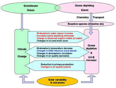Fig. 6 Interactions between ozone depletion and climate change. The sense of the interaction is given by the direction of the arrow. For example, the top horizontal arrow shows examples of how climate change influences ozone depletion and UV-B. Processes that exacerbate the change are in red, processes that ameliorate the change are in blue, and processes that may act both ways are in black (DMS is dimethyl sulphide). Adapted from Clark.²

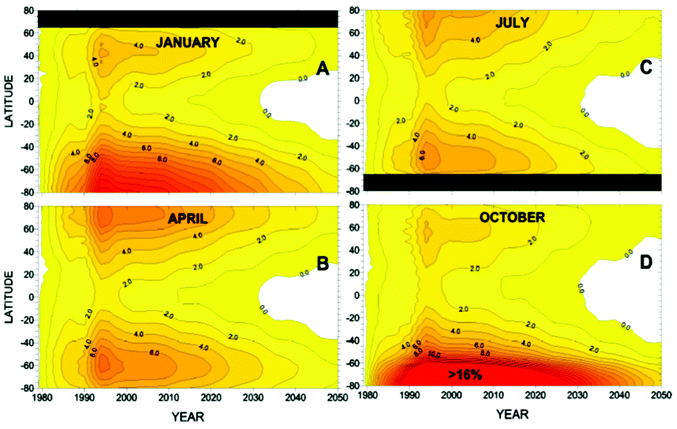Fig. 7 Projection of the departures (in percent) from 1980 UV noontime clear sky irradiance levels between 1979 and 2050 for the months of January (A), April (B), July (C) and October (D).^3,4

Although the outlook for future recovery of ozone and hence future recovery of UV-B is promising, the ozone layer will, as stated in the WMO Scientific Assessment report, remain vulnerable for the next decade or so, even with full compliance to the Montreal Protocol and its amendments and adjustments. Failure to comply would delay or could prevent recovery. UV-B intensities are likely to remain significantly higher than pre-1980 values for the next few years at least.

References

1. V. Fioletov, B. McArthur, J. Kerr and D. Wardle, Long-term variations of UV-B irradiance over Canada estimated from Brewer observations and derived from ozone and pyranometer measurements, J. Geophys. Res., 2001, 106, 23009–23028.
2. E. D. Clark, Ozone depletion and global climate change: linkages and interactive threats to the cetacean environment, in International Whaling Commission Scientific Committee, July 2001, International Whaling Commission, 2001.
3. WMO (World Meterorological Organization), Scientific Assessment of Ozone Depletion, 1998, Global Ozone Research and Monitoring Project, Report No. 44, Geneva, Switzerland, 1999..
4. UNEP, Environmental effects of ozone depletion, 1998 assessment, UNEP Report, Nairobi, p. 192.
5. R. L. McKenzie, G. E. Bodeker, B. J. Connor, P. V. Johnston, M. Kotkamp and W. A. Matthews, Increases in Summertime UV radiation in New Zealand: an update, in Quadrennial Ozone Symposium, eds. R. D. Bojkov and K. Shibasaki, EORC/NASDA, Tokyo, 2000, pp. 237–238.
6. WMO (World Meterorological Organization), Scientific Assessment of Ozone Depletion: 2002 Global Ozone Research and Monitoring Project, Report No. 47, Geneva, Switzerland, 2003.
7. J. F. Abarca, C. C. Casiccia and F. D. Zamorano, Increase in sunburns and photosensitivity disorders at the edge of Antarctic ozone hole, Southern Chile, 1986-2000, J. Am. Acad. Dermatol., 2002, 46, 193–199.
8. M. C. Rousseaux, C. L. Ballaré, C. V. Giordano, A. L. Scopel, A. M. Zima, M. Szwarcberg-Bracchitta, P. S. Searles, M. M. Caldwell and S. B. Diaz, Ozone damage and UVB radiation: impact on plant DNA damage in Southern America, Proc. Nat. Acad. Sci., 1999, 96, 15310–15315.
9. M. M. Caldwell, C. L. Ballaré, J. F. Bornman, S. D. Flint, L. O. Björn, A. H. Teramura, G. Kulandaivelu and M. TeviniTerrestrial ecosystems, increased solar ultraviolet radiation and interactions with other climatic change factors, Photochem. Photobiol. Sci., 2003, in press.
10. G. E. Bodeker, J. C. Scott, K. Kreher and R. L. McKenzie, Global ozone trends in potential vorticity coordinates using TOMS and GOME intercompared against the Dobson networks: 1978-1998, J. Geophys. Res., 2001, 106, 23029–23042.
11. E. C. Weatherhead, G. C. Reinsel, G. C. Taio, C. H. Jackman, L. Bishop, S. M. Hollandsworth Frith, J. DeLuisi, T. Keller, S. J. Oltmans, E. L. Fleming, D. J. Wuebbles, J. B. Kerr, A. J. Miller, J. Herman, R. McPeters, R. M. Nagatani and J. E. Frederick, Detecting the recovery of total column ozone, J. Geophys. Res., 2000, 105, 22201–22210.
12. J. F. Abacra and C. C. Caisccia, skin cancer and ultraviolet-B radiation under the Antactic ozone hole: Southern Chile, 1987–2000, Photoderm. Photoimmunol. Photomed., 2002, 18, in press.
13. S. B. Diaz, G. Deferrari, C. R. Booth, D. Martinioni and A. Oberto, Solar irradiances over Ushuaia (54.49°S, 68.19°W) and San Diego (32.45°N, 117.11°W) geographical and seasonal variation, J. Atmos. Solar-Terr. Phys., 2001, 63, 309–320.
14. A. Cede, E. Luccini, L. Nuñez, R. D. Piacentini and M. Blumthaler, Monitoring of erythemal irradiance in the Argentina ultraviolet network, J. Geophys. Res., 2002, in press.
15. S. Madronich, R. L. McKenzie, L. O. Björn and M. M. Caldwell, Changes in biologically-active ultraviolet radiation reaching the Earth's surface, J. Photochem. Photobiol. B., 1998, 46, 5–19.
16. WMO, Report of the WMO-WHO Meeting of Experts on Standardization of UV Indices and their Dissemination to the Public, WMO Report No. Les Diablerets, Switzerland, 21–24 July 1997, p. 187.
17. M. Ilyas, A. Pandy and S. I. S. Hassan, UV-B radiation at Penang, Atmospheric Research, 1999, 51, 141–152.
18. R. L. McKenzie, P. V. Johnston, D. Smale, B. Bodhaine and S. Madronich, Altitude effects on UV Spectral Irradiance deduced from measurements at Lauder, New Zealand and at Mauna Loa Observatory, Hawaii., J. Geophys. Res., 2001, 106, 22845–22860.
19. A. F. Bais, B. G. Gardiner, H. Slaper, M. Blumthaler, G. Bernhard, R. L. McKenzie, A. R. Webb, G. Seckmeyer, B. Kjeldstad, T. Koskela, P. Kirsch, J. Groebner, J. B. Kerr, S. Kazadzis, K. Lesczynski, D. Wardle, C. Brogniez, W. Josefsen, D. Gillotay, H. Reinen, P. Weihs, T. Svenoe, P. Eriksen, F. Kuik and A. Redondas, SUSPEN intercomparison of ultraviolet spectroradiometers, J. Geophys. Res., 2001, 106, 12509–12526.
20. J. R. Slusser, J. Gibson, D. S. Bigelow, D. Kolinski, P. Disterhoft, K. Lantz and A. Beaubien, Langley method of calibrating UV filter radiometers, J. Geophys. Res., 2000, 105, 4841–4849.
21. J. Gröbner, R. Vergas, V. E. Cachorro, D. V. Henriques, K. Lamb, A. Redondas, J. M. Vilaplana and D. Rembges, Intercomparison of aerosol optical depth measurements in the UVB using Brewer spectrophotometers and a Li-Cor spectrophotometer, Geophys. Res. Lett., 2001, 28, 1691–1694.
22. J. P. Diaz, F. J. Exposito, C. J. Torres, V. Carreno and A. Redondas, Simulation of mineral dust effects on UV radiation levels, J. Geophys. Res., 2000, 105, 4979–4991.
23. V. W. J. H. Kirchhoff, A. A. Silva, C. A. Costa, N. Paes Leme, H. G. Pavao and F. Zaratti, UV-B Optical Thickness Observations of the Atmosphere, J. Geophys. Res., 2001, 106, 2963–2973.
24. F. Zaratti, R. Forno, J. Garcia and M. Andrade, Erythemally-weighted UV-B variations at two high altitude locations, J. Geophys. Res., 2002, in press.
25. D. Meloni, G. R. Casale, A. M. Siani, S. Palmieri and F. Cappellani, Solar UV dose patterns in Italy, Photochem. Photobiol., 2000, 71, 681–690.
26. V. L. Orce and E. W. Helbling, Latitudinal UVR-PAR measurements in Argentina: extent of the ‘ozone hole’, Global and Planetary Change, 1997, 15, 113–121.
27. S. Cabrera, S. Bozzo and H. Fuenzalida, Variations in UV radiation in Chile, Photochem. Photobiol., 1995, B28, 137–142.
28. J. Gröbner, A. Albold, M. Blumthaler, T. Cabot, A. De la Casiniere, J. Lenoble, T. Martin, D. Masserot, M. Müller, R. Philipona, T. Pichler, E. Pougatch, G. Rengarajan, D. Schmucki, G. Seckmeyer, C. Sergent, M. L. Touré and P. Weihs, Variability of spectral solar ultraviolet irradiance in an Alpine environment, J. Geophys. Res., 2000, 105, 26991–27003.
29. C. Varotsos, D. Alexandris, G. Chronopoulos and C. Tzanis, Aircraft observations of the solar ultraviolet irradiance throughout the troposphere, J. Geophys. Res., 2001, 106, 14843–14854.
30. R. L. McKenzie, K. J. Paulin and S. Madronich, Effects of snow cover on UV irradiance and surface albedo: A case study, J. Geophys. Res., 1998, 103, 28785–28792.
31. K. Minschwaner, New observations of ultraviolet radiation and column ozone from Socorro, New Mexico, Geophys. Res. Lett., 1999, 26, 1173–1176.
32. M. Degünther, R. Meerkötter, A. Albold and G. Seckmeyer, Case study on the influence of inhomogeneous surface albedo on UV irradiance, Geophys. Res. Lett., 1998, 25, 3587–3590.
33. M. Degünther and R. Meerkötter, Influence of inhomogeneous surface albedo on UV irradiance: Effect of a stratus cloud, J. Geophys. Res., 2000, 105, 22755–22762.
34. K. F. Evans, The spherical harmonics discrete ordinate method for three-dimensional atmospheric radiative transfer, J. Atmos. Sci., 1998, 55, 429–446.
35. D. W. Mueller, Jr and A. L. Crosbie, Three-dimensional radiative transfer with polarization in a multiple scattering medium exposed to spatially varying radiation, J. Quant. Spectros. Radiat. Transfer, 1997, 57, 81–105.
36. W. O'Hirok and C. Gautier, A three-dimensional radiative transfer model to investigate the solar radiation within a cloudy atmosphere. part I: Spatial effects, J. Atmos. Sci., 1998, 55, 2162–2179.
37. W. O'Hirok and C. Gautier, A three-dimensional radiative transfer model to investigate the solar radiation within a cloudy atmosphere. part II: Spectral effects, J. Atmos. Sci., 1998, 55, 3065–3076.
38. R. L. McKenzie, K. J. Paulin, G. E. Bodeker, J. B. Liley and A. P. Sturman, Cloud cover measured by satellite and from the ground: relationship to UV radiation at the surface, Int. J. Remote Sens., 1998, 19, 2969–2985.
39. J. Chen, B. E. Carlson and A. D. Del Genio, Evidence for strengthening of the tropical general circulation in the 1990s, Science, 2002, 295, 838–841.
40. A. di Sarra, M. Cacciani, P. Chamard, C. Cornwall, J. J. DeLuisi, T. Di Iorio, P. Disterhoft, G. Fiocco, D. Fuá and F. Monteleone, Effects of desert dust and ozone on the ultraviolet irradiance: observations at the Mediterranean island of Lampedusa during PAUR II, J. Geophys. Res., 2002, 107, in press.
41. L. R. Acosta and W. F. J. Evans, Design of the Mexico City UV monitoring network: UV-B measurements at ground level in the urban environment, J. Geophys. Res., 2000, 105, 5017–5026.
42. B. N. Wenny, V. K. Saxena and J. E. Frederick, Aerosol optical depth measurements and their impact on surface levels of ultraviolet-B radiation, J. Geophys. Res., 2001, 106, 17311–17319.
43. M. Z. Jacobson, Global direct radiative forcing due to multicomponent anthropogenic and natural aerosols, J. Geophys. Res., 2001, 106, 1551–1568.
44. R. L. McKenzie, G. Seckmeyer, A. Bais and S. Madronich, Satellite retrievals of Erythemal UV dose compared with ground-based measurements at Northern and Southern mid-latitudes, J. Geophys. Res., 2001, 106, 24051–24062.
45. M. Ilyas, A. Pandy and M. S. Jaafar, Changes to the surface level solar ultraviolet-B radiation due to haze perturbation, J. Atmos. Chem., 2001, 40, 111–121.
46. J. R. Herman, P. K. Bhartia, O. Torres, C. Hsu, C. Seftor and E. Celarier, Global distribution of UV-absorbing aerosols from Nimbus 7/TOMS data, J. Geophys. Res., 1997, 102, 16911–16922.
47. R. L. McKenzie, K. Paulin and M. Kotkamp, Erythemal UV irradiances at Lauder New Zealand: relationship between horizontal and normal incidence, Photochem. Photobiol., 1997, 66, 683–689.
48. A. R. Webb, P. Weihs and M. Blumthaler, Spectral UV irradiance on vertical surfaces: a case study, Photochem. Photobiol., 1999, 69, 464–470.
49. R. E. Shetter and M. Müller, Photolysis frequency measurements using actinic flux spectroradiometry during the PEM-Tropics Mission: instrumentation description and some results, J. Geophys. Res., 1999, 104, 5647–5662.
50. A. Hofzumahaus, A. Kraus and M. Müller, Solar actinic flux spectroradiometry: a technique measuring photolysis frequencies in the atmosphere, Appl. Opt., 1999, 38, 4443–4460.
51. S. Kazadzis, A. F. Bais, D. Balis, C. S. Zerefos and M. Blumthaler, Retrieval of downwelling UV actinic flux density spectra from spectral measurements of global and direct solar UV irradiance, J. Geophys. Res., 2000, 105, 4857–4864.
52. R. L. McKenzie, P. V. Johnston, A. Hofzumahaus, A. Kraus, S. Madronich, C. Cantrell, J. Calvert and R. Shetter, Relationship between photolysis frequencies derived from spectroscopic measurements of actinic fluxes and irradiances during the IPMMI campaign, J. Geophys. Res., 2002, 107, in press.
53. A. R. Webb, R. Kift, S. Theil and M. Blumthaler, An empirical method for the conversion of spectral UV irradiance measurements to actinic flux data, Atmos. Environ., 2002, 36, 4397–4404.
54. N. Y. Chubarova and Y. I. Nezval, Thirty year variability of UV irradiance in Moscow, J. Geophys. Res., 2000, 105, 12529–12539.
55. J. Borkowski, Homogenisation of the Belsk UV-B Series (1976-1997) and Trend Analysis, J. Geophys. Res., 2000, 105, 4873–4878.
56. R. L. McKenzie, B. J. Connor and G. E. Bodeker, Increased summertime UV observed in New Zealand in response to ozone loss, Science, 1999, 285, 1709–1711.
57. C. Zerefos, D. S. Balis, A. F. Bais, D. Gillotay, P. C. Simon, B. Mayer and G. Seckmeyer, Variability of UV-B at four stations in Europe, Geophys. Res. Lett., 1997, 24, 1363–1366.
58. C. Zerefos, C. Meleti, D. S. Balis, K. Tourpali and A. F. Bais, Quasibiennial and longer-term changes in clear-sky UV-B solar irradiance, Geophys. Res. Lett., 1998, 25, 4345–4348.
59. J. R. Herman, R. D. Piacentini, J. Ziemke, E. Celarier and D. Larko, Interannual variability of ozone and UV-B ultraviolet exposure, J. Geophys. Res., 2000, 105, 29189–29193.
60. S. Diaz, G. Deferrari, D. Martinioni and A. Oberto, Regression analysis of biologically effective integrated irradiance versus ozone, clouds and geometric factors., J. Atmos. Sol.-Terr. Phys., 2000, 62, 629–638.
61. M. Huber, M. Blumthaler and J. Schreder, Effect of ambient temperature and internal relative humidity on spectral sensitivity of UV detectors, in SPIE 46th Annual Meeting, eds J. Slusser, J. Herman and W. Gao, SPIE, Washington DC, 2002, vol. 4482, pp. 187–193.
62. J. Kaurola, P. Taalas, T. Koskela, J. Borkowski and W. Josefsson, Long-term variations of UV-B doses at three stations in northern Europe, J. Geophys. Res., 2000, 105, 20813–20820.
63. P. N. den Outer, H. Slaper, J. Matthijsen, H. A. J. M. Reinen and R. Tax, Variability of ground-level ultraviolet: model and measurement, Radiat. Prot. Dosimetry, 2000, 91, 105–110.
64. L. Gantner, P. Winkler and U. Kohler, A method to derive long-term time series and trends of UV-B radiation (1968-1997) from observations at Hohenpeissenberg (Bavaria), J. Geophys. Res., 2000, 105, 4879–4888.
65. J. Verdebout, A method to generate surface UV radiation maps over Europe using GOME, Meteosat, and ancillary geophysical data, J. Geophys. Res., 2000, 105, 5049–5058.
66. P. M. Udelhofen, P. Gies, C. Roy and W. J. Randel, Surface UltraViolet (UV) radiation over Australia, 1979-1992: effects of ozone and cloud cover changes on variations of UV radiation., J. Geophys. Res., 1999, 104, 19135–19159.
67. J. R. Ziemke, S. Chandra, J. Herman and C. Varotsos, Erythemally weighted UV trends over northern latitudes derived from Nimbus 7 TOMS measurements, J. Geophys. Res., 2000, 105, 7373–7382.
68. J. R. Herman, D. Larko, E. Celarier and J. Ziemke, Changes in the Earth's UV Reflectivity from the Surface, Clouds and Aerosols, J. Geophys. Res., 2001, 106, 5353–5368.
69. IPCC, Climate Change 2001: The Scientific Basis. Contribution of Working Group I to the Third Assessment Report of the Intergovernmental Panel on Climate Change, Cambridge University Press, Cambridge, UK, 2001.
70. P. M. Udelhofen, H. P. Gies and C. R. Roy, Comparison of measurements of surface UVR and TOMS UV exposures over Australia, in SPARC 2000, SPARC, CD/SPARC web page, P/4.18, 2000.
71. A. Arola, S. Kalliskota, P. N. den Outer, K. Edvardsen, G. Hansen, T. Koskela, T. J. Martin, J. Matthijsen, R. Meerkoetter, P. Peeters, G. Seckmeyer, P. Simon, H. Slaper, P. Taalas and J. Verdebout, Assessment of four methods to estimate surface UV radiation using satellite data, by comparison with ground measurements from four stations in Europe, J. Geophys. Res., 2002, 107, in press.
72. R. D. Piacentini, E. Crino, J. S. Flores, J. y. M. Ginzburg, Intercomparison between ground based and TOMS/EP satellite southern hemisphere ozone data. New results, in Proceedings SPARC (Stratospheric Processes and their Role on Climate) 2000, SPARC, CD/SPARC web page, P/2-3.2., 2000..
73. B. Rognerud and I. Isaksen, Model calculations of stratospheric ozone recovery, in NDSC Conference, Network for the Detection of Stratospheric Change, 2001.
74. L. K. Randeniya, P. F. Vohralik and I. C. Plumb, Stratospheric ozone depletion at northern mid latitudes in the 21st century: The importance of future concentrations of greenhouse gases nitrous oxide and methane, Geophys. Res. Lett., 2002, 29, in press.
75. J. B. Liley, P. V. Johnston, R. L. McKenzie, A. J. Thomas and I. S. Boyd, Stratospheric NO₂ variations from a long time series at Lauder, New Zealand, J. Geophys. Res., 2000, 105, 11633–11640.
76. C. A. McLinden, S. C. Olsen, M. J. Prather and J. B. Liley, Understanding trends in stratospheric NO_y and NO₂, J. Geophys. Res., 2001, 106, 27787–27793.
77. J. E. Rosenfield, A. R. Douglass and D. B. Considine, The impact of increasing carbon dioxide on ozone recovery, J. Geophys. Res., 2002, 107, in press.
78. D. T. Shindell, D. Rind and P. Lonergan, Increased polar stratospheric ozone losses and delayed eventual recovery owing to increasing greenhouse-gas concentrations, Nature, 1998, 392, 589–592.
79. P. Bunyard, How ozone-depletion increases global warming, The Ecologist, 1999, 29, 85.
80. B. A. Wielicki, T. Wong, R. P. Allan, A. Slingo, J. T. Kiehl, B. J. Soden, C. T. Gordon, A. J. Miller, S.-K. Yang, D. A. Randall, F. Robertson, J. Susskind and H. Jacobowitz, Evidence for large decadal variability in the tropical mean radiative energy budget, Science, 2002, 295, 841–844.
81. P. Taalas, J. Kaurola, A. Kylling, D. Shindell, R. Sausen, M. Dameris, V. Grewe, J. Herman, J. Danski and B. Steil, The impact of greenhouse gases and halogenated species on future solar UV radiation doses., Geophys. Res. Lett., 2000, 27, 1127–1130.
82. D. L. Hartmann, J. M. Wallace, V. Limpasuvan, D. W. J. Thompson and J. R. Holton, Can ozone depletion and global warming interact to produce rapid climate change?, Proc. Nat. Acad. Sci., 2000, 97, 1412–1417.
83. M. P. Baldwin and T. J. Dunkerton, Stratospheric harbingers of anomalous weather regimes, Science, 2001, 294, 581–584.
84. N. Butchart and A. A. Scaife, Removal of chlorofluorocarbons by increased mass exchange between the stratosphere and troposphere in a changing climate, Nature, 2001, 410, 799–802.
85. D.-P. Häder, H. D. Kumar, R. C. Smith and R. C. Worrest, Aquatic ecosystems: effects of increased solar ultraviolet radiation and interactions with other climatic change factors, interactions with other climatic change factorspress, Photochem. Photobiol. Sci., 2003.
86. R. G. Zepp, T. V. Callaghan and D. J. EricksonInteractive effects of ozone depletion and climate change on biogeochemical cycles, Photochem. Photobiol. Sci., 2003, in press.
87. K. H. Rosenlof, S. J. Oltmans, D. Kley, J. M. Russell III, E.-W. Chiou, W. P. Chu, D. G. Johnson, K. K. Kelly, H. A. Michelson, G. E. Nedoluha, E. E. Remsberg, G. C. Toon and M. P. McCormick, Stratospheric water vapor increases over the past half-century, Geophys. Res. Lett., 2001, 28, 195–198.
88. N. Stuber, M. Ponater and R. Sausen, Is the Climate Sensitivity to Ozone Perturbations Enhanced by Stratospheric Water Vapor Feedback?, Geophys. Res. Lett., 2001, 28, 2887–2890.
89. T. Nagashima, M. Takahashi, M. Takigawa and H. Akiyoshi, Future development of the ozone layer calculated by a general circulation model with fully interactive chemistry, Geophys. Res. Lett., 2002, 29, 31–34.
90. V. Ramaswamy, M.-L. Chanin, J. Angell, J. Barnett, D. Gaffen, M. Gelman, P. Keckut, Y. Koshelkov, K. Labitske, J.-J. Lin, R. A. O'Neill, J. Nash, W. Randel, R. Rood, K. P. Shine, M. Shiotani and R. Swinbank, Stratospheric temperature trends: observations and model simulations, Rev. Geophys., 2001, 39, 71–122.
91. D. W. J. Thompson and S. Solomon, Interpretation of recent Southern Hemisphere climate change, Science, 2002, 296, 895–899.
92. A. Fergusson, Ozone depletion and climate change: understanding the linkages, Meteorological Service, Environment Canada Report No. Toronto, p. 34.
93. J. Rozema, B. van Geel, L. O. Björn, J. Lean and S. Madronich, Toward Solving the UV Puzzle, Science, 2002, 296, 1621–1622.
94. T. Egorova, E. V. Rozanov, M. E. Schleisinger, N. G. Andronova, S. L. Malyshev, I. L. Karol and V. A. Zubov, Assessment of the Effect of the Montreal Protocol on Atmospheric Ozone, Geophys. Res. Lett., 2001, 28, 2389–2392.

Footnote

† This article is published as part of the United Nations Environmental Programme: Environmental effects of ozone depletion and its interactions with climate change: 2002 assessment.

---