Manipulation of electroactive polymer film viscoelasticity: the roles of applied potential and frequency †
Mark J. Browna, A. Robert Hillman*a, Stephen J. Martinb, Richard W. Cernosekb and Helen L. Bandeyb
aDepartment of Chemistry, University of Leicester, Leicester, UK LE1 7RH, arh7@le.ac.uk
bMicrosensor Research Division, Sandia National Laboratories, Albuquerque, NM 87185, USA
First published on UnassignedUnassigned22nd December 1999
Abstract
We describe quartz crystal impedance measurements on thin films of poly(3-hexylthiophene) (PHT) electrochemically maintained at different potentials and exposed to propylene carbonate electrolyte solutions. Film shear modulus values, obtained at fixed potentials corresponding to a range of film oxidation states (“doping levels"), show a marked variation of storage and loss moduli ( G′ and G″, respectively). The p-doped film is substantially softer than the undoped film, and G′ and G″ can show maxima at partial p-doping. Even in nominally “equilibrium" experiments (at fixed potential) there is dramatic hysteresis in shear modulus values determined during stepwise doping and undoping. This general pattern of behaviour is observed at a range of frequencies, corresponding to the fundamental frequency (10 MHz) and higher harmonics (30 MHz to 110 MHz). There are substantial increases in shear modulus with increasing frequency for all doping levels, and the loss tangent ( G″/ G′) is frequency dependent. A Voigt model is qualitatively incompatible with these observations, and a Maxwell model can qualitatively explain some features; more sophisticated models are required to provide quantitative explanations. We discuss these observations in terms of potential-driven film ion and solvent population changes. The data are consistent with non-equilibrium film solvent populations for intermediate doping levels, even though the equilibrium ion populations (charge states) may be established. Together, selection of operating frequency, applied potential and time scale offer the prospect of manipulating film viscoelastic parameters in a controllable manner over several orders of magnitude, from “rubbery" to near “glassy" behaviour.
Introduction
Overview
Over the last decade, two major features of electrochemical science have been its contribution to materials science 1 and the application of non-electrochemical physical methods to the study of electrochemical systems and processes. 2–4 The field in which these two activities meet—with profound synergistic effects—is that of modified electrodes, 5,6 involving the deliberately planned construction of interfacial architectures with specified chemical, optical or electrical characteristics. Quite generally, the key to further progress in this area is a better understanding of materials-based issues, notably their design, fabrication and characterization.Here, we explore polymer dynamics within thin electroactive polymer films maintained in electronically conducting or insulating states. The general goals are an understanding of how thin film material characteristics (film shear modulus) respond to (i) their environment (here, a liquid electrolyte) and (ii) external control parameters (here, polymer charge density, as dictated by applied electrochemical potential). This is broadly complementary to the majority of work on such materials, which tends to focus on electronic properties per se. The link is that redox-driven changes in electronic characteristics (“doping" and “undoping") require polymer structural changes that are markedly influenced by polymer dynamics. We therefore see a proper understanding of polymer dynamics as an important prerequisite for the design of polymer-based interfacial modifications. In the context of materials science, it is interesting to note that the importance of bulk viscoelastic characteristics of polymers has long been appreciated, 7,8 to the extent that molecular interpretations of the macroscopic phenomena have been discussed at length. 9 However, the analogous phenomena for thin films of polymers—the focus of this study—have not received such attention.
Polymers as materials for electrode modification
From reviews of this rapidly developing field 5,6 it is clear that polymeric materials offer the greatest opportunities for controlled modification of electrode surfaces. Applications promised by such modified electrodes include electronic devices, optical displays, energy storage/conversion, (bio)chemical sensors of various kinds, corrosion protection and electrocatalysis. As a general result, the vast body of literature in this area (reviewed in references 5 and 6) clearly indicates that successful application is largely a question of materials design, characterization and optimization. In general terms, one requires to know how electroactive species behave within a polymeric environment ( cf. as monomeric entities in free solution) and how the characteristics of the polymer as a thin film, under the influence of applied electrochemical potential, differ from those of bulk material.The material we study here, poly(3-hexylthiophene) (PHT), is a polyheterocycle, of which the most widely studied materials are the parent poly(thiophene) and poly(pyrrole). These so-called “conducting polymers" have attracted enormous research interest 10,11 due to the manner in which one can manipulate their electronic conductivity—and the associated optical characteristics—by (electro)chemical oxidation and reduction (commonly referred to as “doping" and “undoping"). This has prompted their application in lightweight batteries, 12 flexible (“all plastic") transistors 13,14 and display devices. 15,16 Our interest in this area has focused on thiophene-derived materials. It has involved studies of film nucleation and growth phenomena 17,18 and characterization of the resultant films in terms of their electronic properties (using visible, 19 FTIR 20 and ESR 21 spectroscopies) and of the concomitant “dopant" and solvent transfers (using the electrochemical quartz crystal microbalance (EQCM) 22). We also explored manipulation of electron dynamics by substituent effects, through the effect on electronic properties 23 of a fused benzene ring. Here, we explore the effect of a hydrocarbon side-chain on polymer dynamics, through its effect on solvation characteristics.
We have also investigated two-component composite and segregated bilayer structures with spatially controlled characteristics. 24,25In situ neutron reflectivity studies 26 of such structures showed the importance of the spatial distributions of the polymer, solvent and ion components at the interface. 27 Together with the interpretation of our present rheological observations, this issue will inform the future design of interfacial materials.
Thickness shear mode (TSM) devices
One of the many in situ techniques used to study electroactive polymer films is the electrochemical quartz crystal microbalance (EQCM). 28,29 We discuss the details of the technique below, but here comment on the strategic use of the method. The simplest physical situation is a rigid film. Here the EQCM functions as a gravimetric probe: resonant frequency changes, Δ f, are linearly related to film mass changes, Δ M. Under these circumstances, the EQCM has been widely used to monitor redox-driven ion and solvent dynamics and population changes within polymer films. 28,29 In the alternative situation that the film is not rigidly coupled to the crystal, the EQCM is a viscoelastic probe and its response is predominantly a function of polymer dynamics. These two cases are distinguishable on the basis of the crystal admittance, i.e. analysis of the full frequency response in the vicinity of resonance.Much of the reported work, both experimental and theoretical, on TSM devices loaded with viscoelastic films relates to polymer coatings exposed to gaseous environments. This is, at least in part, because a significant application of such devices is in gas phase sensors, e.g. for volatile organic compounds that can permeate and soften the polymer films. 30 That physical situation is relatively simple, since the resonator loading only involves one component; to a first approximation, the gas contributes negligibly to the surface mechanical impedance. The general situation involves exposure to fluids; this is necessarily the case in the electrochemical context we consider here. This brings two complications. First, there is an additional loading. Second, in the more general case that there is significant acoustic deformation across the film, the effects of the film and the fluid are not additive. 31,32 More positively, application in situ allows the use of applied electrochemical potential as a powerful means of manipulating interfacial composition, structure and properties; it is this feature we exploit in this study.
Objectives and scope of the study
The majority of TSM-based studies of polymer films have been rather limited: most commonly they are restricted to qualitative diagnosis of film (non-)rigidity, and there are a few examples of film shear moduli determinations (see below). We adopt a more ambitious approach, with the ultimate objective of a priori control and in situ manipulation of film shear modulus and dynamics. This capability would have direct potential applications in sensing, molecular recognition, controlled release and separation science, as well as indirect generic benefits in interfacial design.The intermediate goal is a systematic understanding of the parameters that govern film shear modulus. Qualitatively, the shear modulus is recognized to depend upon physicochemical parameters which may be intrinsic to the polymer, a feature of its environment or amenable to external control. Our immediate objective is an understanding of the roles of film charge (
Q) and the frequency regime (
 ) in which the system operates. Film charge is a variable of natural choice, since it can be readily manipulated through the applied electrochemical potential (
E): it is a primary driver of film composition—most obviously ion and solvent content—and structure. Operating frequency as a delimiter of film dynamics is much under-explored: the vast majority of studies are based upon TSM device responses at their fundamental frequency, typically 5 or 10 MHz. Here we use higher harmonics to effect simultaneous measurements at a range of frequencies; this is relatively rare for viscoelastic measurements of electroactive polymer films and offers significant novel insights into materials properties.
) in which the system operates. Film charge is a variable of natural choice, since it can be readily manipulated through the applied electrochemical potential (
E): it is a primary driver of film composition—most obviously ion and solvent content—and structure. Operating frequency as a delimiter of film dynamics is much under-explored: the vast majority of studies are based upon TSM device responses at their fundamental frequency, typically 5 or 10 MHz. Here we use higher harmonics to effect simultaneous measurements at a range of frequencies; this is relatively rare for viscoelastic measurements of electroactive polymer films and offers significant novel insights into materials properties.
Film composition (mobile species populations) and structure (polymer configuration) may be under either thermodynamic or kinetic control, according to the electrochemical control function and other experimental parameters. Here we restrict our attention to static measurements at fixed Q( E). Here the film is at redox equilibrium although, as we shall show, the question of equilibrium with regard to non-electrochemical processes (such as solvation and polymer reconfiguration) is more complex. Dynamic electrochemical measurements, for example during a potential scan, represent greater instrumental and interpretational challenges that we will confront in future.
Methodology: the EQCM and crystal impedance
Thickness shear mode resonators, exemplified by AT-cut quartz crystal oscillators, display frequency responses that reflect their ambient medium. The solids, liquids or gases to which they are exposed impose a surface mechanical impedance, ZS, on the resonator. Through the piezoelectric coupling constant, this mechanical impedance is manifested as an electrical impedance that can be measured in a conventional manner. Interpretation of the impedance is commonly effected through equivalent circuit models, in which capacitive, inductive and resistive elements, respectively, represent elastic energy storage, kinetic energy storage (inertial mass) and energy dissipation.The simplest condition is that involving no energy loss. This corresponds to a surface mass loading rigidly coupled to the resonator that moves synchronously with it. For this case, Sauerbrey showed 33 that the resonant frequency change (Δ f) of a quartz crystal oscillator in response to a change in the film areal density (Δ M/g cm –2) is given by eqn. (1),
 | (1) |
where ρq is the density of the crystal, vq is the wave velocity within it, and f0 is the initial frequency (in our case, 10 MHz). This is the basis of the quartz crystal microbalance (QCM) technique, widely used for monitoring deposition from the gas phase onto solid substrates. 34
When the resonator is exposed to a liquid, viscous losses damp the resonance, but Kanazawa
35 and Bruckenstein
36 showed that this energy loss is not so severe as to preclude oscillation. The TSM launches into the liquid an acoustic wave with a decay length,
 , where
ηL and
ρL are the liquid viscosity and density. The effective inertial/viscous coupling to the liquid results in a frequency shift (decrease) and a contribution to (increase in) the resonant resistance. However, these phenomena still allow one to use the exciting electrode as the working electrode under potential control in an electrochemical cell. This is the basis of the EQCM, which acts as a gravimetric probe of the surface population(s) of rigid polymer, together with its entrained ions and solvent.
, where
ηL and
ρL are the liquid viscosity and density. The effective inertial/viscous coupling to the liquid results in a frequency shift (decrease) and a contribution to (increase in) the resonant resistance. However, these phenomena still allow one to use the exciting electrode as the working electrode under potential control in an electrochemical cell. This is the basis of the EQCM, which acts as a gravimetric probe of the surface population(s) of rigid polymer, together with its entrained ions and solvent.
Interpretation of EQCM data according to eqn. (1) is entirely reliant upon the film being rigidly coupled to the crystal. One technique for (dis)proving this is the crystal impedance method, in which one determines the complete frequency response in the vicinity of resonance. Purely gravimetric effects result in frequency shifts (described by the Sauerbrey equation) and no change in peak admittance. They are represented as changes in inductance, but not resistance, in equivalent circuit models. Physically, the film oscillates synchronously with the crystal; films with shear moduli on the order of 10 10 dyn cm −2 show this behaviour. Contrastingly, viscoelastic changes result in changes in peak admittance, as a consequence of the change in energy loss to the ambient medium. They are represented as changes in resistance in equivalent circuit models. Physically, there is an acoustic deformation across the film, i.e. it does not oscillate synchronously with the crystal; films with shear moduli on the order of 10 6–10 8 dyn cm –2, characteristic of rubbery materials, typically show this behaviour.
A special case of a viscoelastically-driven response is film resonance, when the film thickness corresponds to one quarter of the acoustic wavelength. This results in a dramatic change in the coupling and energy transfer between the resonator and the film. Although recognized for some time in the context of films exposed to gases, 37 film resonance in the presence of liquids has only recently been reported. 38–40
The presence/absence of variations in resonant resistance has been used as a qualitative diagnostic of film (non-)rigidity for a range of polymer films. 41–47 The next step, upon which this paper focuses, is quantitative interpretation of crystal impedance responses in terms of physically meaningful parameters, specifically the complex shear modulus, G = G′ + jG″, where G′ and G″, respectively, are the polymer film storage and loss moduli.
One aspect of this topic, which predominated in earlier studies, concerned polymer film-coated resonators exposed to gaseous media; this included both theoretical models 48,49 and mechanistic experimental studies. 37,50–53 Later works considered multiple non-piezoelectric layers, 31,54 and recently a generalized treatment has been presented. 32 Experimentally, the primary focus has been the fundamental study of polymer films exposed to bulk liquid media, 38–40,55–58 although some liquid phase sensor-oriented applications have been described. 59–62
The model we employ here is derived from our generalized treatment for multiple non-piezoelectric layers. 32 We consider (see Fig. 1) a finite viscoelastic layer (of thickness hf, density ρf and shear modulus G = G′ + jG″) exposed to a bulk fluid (of viscosity ηL and density ρL). We take account of surface roughness, and polymer trapped within surface features, by inclusion of a thin layer of “ideal mass". This accords with the generally recognized 58,63,64 fact that intrinsically viscoelastic (or viscous) material entrapped within surface features will behave as rigidly coupled material.
 | ||
| Fig. 1 Schematic view of the three-component loading model underlying eqn. (5) and used to interpret the crystal impedance data. The lines illustrate the standing acoustic wave in the crystal and the acoustic wave that is launched into the system, wherein it becomes progressively damped as one moves out into the polymer film and the solution. | ||
For the individual loading elements, the surface mechanical impedances 32,58 are given by eqn. ( 2)
 | (2) |
for the ideal mass layer (where ρS is the mass per area contributed by the layer);
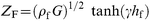 | (3) |
by
eqn. (3) for the viscoelastic film (where the shear wave propagation constant (
 ); and
 | (4) |
by eqn. (4) for the electrolyte solution (a Newtonian fluid). In each of the above equations, ω = 2 πf (where f is the operating frequency of the measurement) and j = √(−1).
For such a composite system, the impedance at the resonator surface is not simply the sum of those for the individual layers. 32,58 Each layer in which there is an acoustic phase shift causes a transformation of the impedance contributed by layers more distant from the resonator. One can show 31,32,58 that the surface mechanical impedance for the configuration of Fig. 1 is given by eqn. (5)
 | (5) |
where
 .
.
Modeling viscoelastic behaviour of polymers
Constitutive relations
The goal of this section is to derive a model for the polymer's viscoelastic properties as a function of excitation frequency and oxidation (doping) state. The frequency dependence of modulus is modeled by postulating a constitutive relation, i.e., a relationship between stress ( T) and strain ( S) for a material. When a stress is applied to a material, it results in a combination of elastic deformation (reversible energy storage) and dissipation (irreversible energy loss).Purely elastic deformation results in a constitutive relationship given by Hooke's law: T = µS, where µ is the stiffness of the material. This constitutive relationship is commonly represented by an ideal spring. Purely viscous dissipation arises in a Newtonian fluid, described by the constitutive relationship: T = η(d S/d t), where η is the viscosity, t is time, and d S/d t is the strain rate. This is commonly represented by an ideal “dashpot"—a plunger in a fluid. Polymers exhibit both elastic deformation and viscous dissipation, i.e. are viscoelastic.
The viscoelastic behaviour of a polymer can be approximated by various combinations of springs and dashpots, 8 which each give rise to a unique frequency dependence that can be tested experimentally. The simplest approximations that account for both energy storage and dissipation are a series and a parallel combination of a spring and dashpot.
The Voigt model, Fig. 2a, consists of a parallel combination of the spring and dashpot. This implies equal strains across the two elements, while the stresses are additive, which gives rise to the constitutive relation given in eqn. (6)
 | ||
| Fig. 2 Two-element models leading to constitutive relationships for a polymer: (a) Voigt model, (b) Maxwell model. | ||
 | (6) |
where we have explicitly shown that µ and η refer to a film, via the subscript “f", and G is the resulting complex shear modulus. We can express eqn. (6) in the form of eqn. (7)
 | (7) |
where τ = ηf/ µf is a characteristic relaxation time.
The Maxwell model, Fig. 2b, consists of a series combination of the spring and dashpot. This implies that the stresses across each element are the same, while the strains are additive, which gives rise to the constitutive relation given in eqn. (8)
 | (8) |
With a little algebraic manipulation, we can express eqn. (8) in the form of eqn. (9)
 | (9) |
where the symbols have the same significance as above. For each model, G′ and G″, respectively, are identified with the real and imaginary components of eqn. (7) and (9).
Frequency dependence of shear modulus
The Voigt model predicts a very simple frequency dependence, illustrated in Fig. 3a. The storage modulus is independent of frequency ( G′ = µf), while the loss modulus is proportional to frequency ( G″ = ωηf). | ||
| Fig. 3 Frequency dependences of the storage ( G′) and loss ( G″) moduli predicted by (a) the Voigt model and (b) the Maxwell model. | ||
The Maxwell model predicts a somewhat more complicated frequency dependence, illustrated in Fig. 3b. G′ increases monotonically with frequency, saturating at µf, while G″ goes through a peak (maximum value of µf/2) at ωτ = 1. The low frequency ( ωτ ≪ 1) limiting characteristics are quadratic and linear, respectively, for G′ and G″.
The Maxwell model exhibits behaviour more in line with that commonly observed with a polymer. When a polymer is deformed slowly (compared with the time for segmental chain motion), applied stress is taken up by inter-chain movements, i.e., chains slip past one another. This results in viscous dissipation predominating. When the polymer is deformed rapidly, the chains do not have time to re-orient and move past one another; instead, the strain is taken up by deformation of the individual polymer chains. This results in elastic storage predominating. The Maxwell model gives both of these extremes. At low frequencies (when ωτ ≪ 1) viscous dissipation predominates, while at high frequencies (when ωτ ≫ 1) elastic storage predominates. The frequency dependence of the Maxwell model, shown in Fig. 3b, illustrates a glass-to-rubber transition. Low ωτ gives a low storage modulus ( G′), corresponding to a rubbery polymer, and high ωτ gives a large G′, corresponding to a glassy polymer. Between these limits, the elastic and viscous components match, so that G″ is maximum. (This model can be improved to more closely describe the behaviour in the rubbery regime by adding, in parallel to the Maxwell elements, a spring with a modulus that matches that of a rubbery polymer, approximately 10 7 dyn cm −2.)
Solvent effects
A central feature of any in situ electrochemical experiment is the presence of solvent. It is generally acknowledged that solvent penetrates surface-immobilized polymer films, although the extent to which this occurs, the rate at which it happens and the effects it induces are the subject of debate. We therefore need to consider what effect solvent permeation might have on the polymer films we consider here, as manifested through film viscoelastic characteristics.The glass-to-rubber transition exhibited by the Maxwell model can also be induced by varying relaxation time ( τ) at fixed frequency (effectively, ω). Since τ = ηf/ µf, this parameter can be controlled either through the modulus or viscosity of the polymer. It is well known 7,8 that the glass-to-rubber transition in a glassy polymer can be induced either by increasing the temperature or through solvent absorption. In either case, the polymer viscosity—and hence τ—is decreased, thereby inducing a glass-to-rubber transition. The glassy regime may thus be associated with high frequency, low temperature, or pure (solvent-free) polymer. The rubbery regime may be associated with low frequency, high temperature, or high solvent content.
The effect of solvent absorption can be modeled by postulating 7 that polymer viscosity (as represented by the viscous element ηf in the Maxwell model) varies because incorporated solvent contributes “free volume" to the material. This free volume “lubricates" the interaction between polymer chains, thereby decreasing the viscosity. If the amount of free volume increases linearly with the amount of incorporated solvent, then the observed viscosity in the presence of solvent incorporation ( ηf) will be decreased from its value ( ηf,0) in the absence of solvent according to eqn. (10)
 | (10) |
where k is a plasticization constant and VS is the volume fraction of the absorbed solvent. According to the Maxwell model, this decrease in ηf causes the relaxation time ( τ) to decrease and (for ωτ < 1) G′ and G″ to decrease.
Experimental
The instrumentation and electrochemical cell have been described elsewhere. 39,40,58 Crystal impedance spectra were recorded using a Hewlett-Packard HP8751A network analyzer, connected via a 50 Ω coaxial cable to a HP87512A transmission/reflection unit. Measurements were made sequentially, at fixed potential at the fundamental (10 MHz) and at the third, fifth, seventh, ninth and eleventh harmonics (30 through 110 MHz). The crystals were 10 MHz AT-cut quartz crystals, coated with Au electrodes with piezoelectrically and electrochemically active areas, respectively, of 0.21 cm 2 and 0.23 cm 2; use of polished crystals minimized surface roughness effects. 58 A conventional three electrode electrochemical cell was employed: one of the Au electrodes of the crystal was the working electrode, a Pt gauze was the counter electrode, and a Ag + (0.01 mol dm −3)/Ag electrode was the reference electrode. The cell was thermostatted at 25![[thin space (1/6-em)]](https://www.rsc.org/images/entities/char_2009.gif) °C.
°C.
PHT film deposition has been described previously. 39 The deposition solution contained 3.7 mmol dm −3 3-hexylthiophene (HT) (Aldrich) and 0.1 mol dm −3 tetraethylammonium hexafluorophosphate (TEAPF 6) (Aldrich, >99%) in propylene carbonate. A potentiodynamic program was used, involving a voltage interval of 0.0–1.5 V in cycle 1, and of 0.0–1.2 V in subsequent cycles. The potential scan rate ( v) was 20 mV s −1. Film thickness was controlled via the number of potential cycles, here six. Together with the doping level ( n = 0.35), the integral ( Qred) of the current response for the PHT film reduction in each polymerization cycle provided a dynamic coulometric assay of polymer coverage ( Γ).
Following deposition, the Au/PHT electrodes were transferred to background electrolyte solution (0.1 mol dm −3 tetraethylammonium hexafluorophosphate in propylene carbonate). Cyclic voltammetry (0.0–0.9 V, scan rate 2 mV s −1; see Fig. 4, below) indicated chemically reversible redox behaviour. Static potentials were applied to the film, ascending from 0 V (at 0.0, 0.4, 0.5, 0.6 and 0.9 V) then descending from 0.9 V (at 0.9, 0.6, 0.4, 0.2 and 0.0 V). The film was held at each potential for 2 min before crystal impedance measurements were recorded at each harmonic.
 | ||
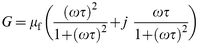
| Fig. 4 Cyclic voltammogram of a PHT film ( Γ = 0.22 µmol cm −2) exposed to 0.1 mol dm −3 TEAPF 6–propylene carbonate. Scan rate: 2 mV s −1. At scan rates v ≤ 20 mV s −1 peak currents are linear with scan rate, indicating complete redox conversion. | ||
The mechanics of fitting experimental data to eqn. (5), and thus extracting film parameters, have been described elsewhere. 32,58 We determined crystal parameters via measurements on the bare crystal in air, then liquid parameters via measurements on the bare crystal in the electrolyte, and finally film parameters via measurements on the polymer-coated crystal in the electrolyte. Thus, we never fit an excessive number of parameters on the basis of a single data set. An important feature of the use of harmonics, discussed below, is that the number of measured parameters increases faster than the number of fitted parameters. Specifically, although the shear modulus components may be frequency dependent, the film thickness and density are not. This allows the choice of either holding these latter two parameters constant (thereby decreasing the number of fitted parameters) or of allowing them to “float" in measurements at different frequencies (thereby using their constancy—or otherwise—as a measure of uniqueness of fit).
Results
Raw spectra
Fig. 4 shows a typical voltammogram for a PHT film upon redox cycling in 0.1 mol dm −3 TEAPF 6–propylene carbonate. It shows all the characteristics generally found for poly-(thiophene)-type films, 10 with p-doping/undoping (see Scheme 1) occurring during the positive-/negative-going half-cycle. The conditions under which this voltammogram was obtained, primarily slow potential scan rate, allow complete redox conversion of the film. This is signified by linearity of peak currents with potential scan rate for v ≤ 20 mV s −1. Consequently, we were able to use the integrated peak currents as a reliable measure of the polymer coverage, Γ = Q/ nFA, with the doping level taken to be n = 0.35. 39 | ||
| Scheme 1 PHT redox chemistry. | ||
Fig. 5 and 6 show representative crystal impedance spectra for this PHT film as a function of the applied (fixed) potential. Within each figure are two sets of spectra, acquired at progressively increasing and progressively decreasing applied potentials, i.e. during “doping" of a fully reduced (uncharged) PHT film and during “undoping" of a fully oxidized (positively charged) PHT film. In the interests of brevity, we do not show figures for all the harmonics acquired: the fundamental and eleventh harmonic are chosen to represent the spread of behaviour occasioned by choice of frequency regime.
 | ||
| Fig. 5 Raw crystal impedance spectra for the PHT film of Fig. 4 exposed to 0.1 mol dm −3 TEAPF 6–propylene carbonate. Open symbols: data acquired at progressively more positive applied potentials, commencing at 0 V; filled symbols: data acquired at progressively more negative applied potentials, commencing at 0.9 V. Data taken at fundamental frequency (nominally 10 MHz). The asterisk adjacent to one of the spectra refers to Fig. 10. | ||
 | ||
| Fig. 6 Raw crystal impedance spectra for the film of Fig. 5 taken under identical conditions, except at the eleventh harmonic (nominally 110 MHz). | ||
We make four qualitative observations. First, there are obvious viscoelastic changes: the doped polymer is associated with greater energy loss (lower peak admittance). Second, these effects are a function of frequency. Third, in all data sets (other films, harmonics and choices of potential program) we see “asymmetry" of the crystal frequency responses during the oxidative and reductive half cycles. This will be a key discussion point later in the text. Fourth, appropriate combinations of film thickness, applied potential and frequency lead to film resonance effects, 39 in which the peak admittance and frequency show dramatic variations. To illustrate the breadth of behaviour observed, we have elected to show here data that are ( Fig. 6)/are not ( Fig. 5) complicated by these phenomena; we are able to handle such effects within our model. 31,32,39
Fig. 7 and 8, respectively, summarize some of the key features of Fig. 5 and 6, through the potential variations of resonant conductance ( Fig. 7a and 8a) and resonant frequency ( Fig. 7b and 8b). The most prominent features of the data are the pronounced hysteresis in all cases, and its appearance in “reverse" fashion for the 110 MHz resonant frequency data. The latter is a consequence of resonance effects, which have been shown 39 to cause a reversal in the normal trends of resonant frequency and peak admittance.
 | ||
| Fig. 7 Peak conductance ( Umax; panel a) and peak frequency ( fmax; panel b) variations with applied potential at 10 MHz; data taken from Fig. 5. Open (filled) symbols represent data acquired during increasing (decreasing) fixed potential sequence. Lines connecting adjacent points are merely a guide to the eye. | ||
 | ||
| Fig. 8 Peak conductance ( Umax; panel a) and peak frequency ( fmax; panel b) variations with applied potential at 110 MHz; data taken from Fig. 6. Open (filled) symbols represent data acquired during increasing (decreasing) fixed potential sequence. Lines connecting adjacent points are merely a guide to the eye. | ||
Since the responses are not single valued with potential, it is immediately clear that global equilibrium is not established, even on the rather extended time scales employed here. The question is whether this represents failure to establish equilibrium of the redox state or of other associated processes. Fig. 9 shows a plot of the injected charge density ( Q) as a function of potential for the experiments of Fig. 5 and 6 (and their analogs at intervening harmonics). Whilst there is some hysteresis, i.e. redox equilibrium is not fully established, the extent of this hysteresis is nowhere near as marked as in the viscoelastic responses. We therefore conclude that the film viscoelastic characteristics are under effective control by intrinsically non-electrochemical processes that are a consequence of its electrochemical oxidation/reduction.
 | ||
| Fig. 9 Plot of charge density ( Q) vs. potential ( E) for the PHT film of Fig. 4–8. The charge data were acquired by progressively incrementing the potential in the intervals used for the experiments of Fig. 5–8. Open (filled) symbols represent data acquired during increasing (decreasing) fixed potential sequence. | ||
Fitted data
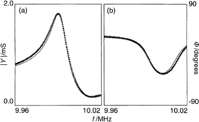 | ||
| Fig. 10 Typical fits to the amplitude (| Y|; panel a) and phase ( Φ; panel b) data for a crystal impedance spectrum. The data (points) are taken from the spectrum marked with * in Fig. 5. The lines represent the best fits. | ||
Some general observations are appropriate with regard to the reliability (reproducibility) of G′ and G″ values. We were always able to get reliable (reproducible) values of the larger component of G, regardless of the starting values used to seed the fitting algorithm. However, the reliability of the smaller component was dependent upon the relative values of G′ and G″, i.e. the loss tangent. When 0.1 ≥ G″/ G′ ≥ 10, both components were reliably obtainable. However, outside this range, the smaller component could not be obtained with any certainty; all we could conclude was that it was more than an order of magnitude smaller than the larger component.
 | ||
| Fig. 11 Fitted film density values as functions of applied potential for the data of Fig. 5 (□, ■) and its third (△, ▲), fifth (▽, ▼) and seventh (◊,♦) harmonic analogs. Open (filled) symbols represent data acquired during increasing (decreasing) fixed potential sequence. | ||
 | ||
| Fig. 12 Fitted film thickness values as functions of applied potential for the data of Fig. 5 and its third, fifth and seventh harmonic analogs. Symbols as in Fig. 11. | ||
Naturally, the film composition and dimensions—here represented by film density and thickness—are independent of the excitation frequency with which we elect to probe them (although the same is not true of the film modulus; see below). (The only apparent violation of this would be the situation where the range of frequencies employed, taking account of their effect on G, and the film thickness were such that one moved between the acoustically “thin" and acoustically “thick" cases within a single data set. In the latter case, corresponding to hf ≫ ω–1( G/ ρf) 1/2, the TSM would perceive the film as being of “infinite" extent; we did not explore this less interesting regime.) As the data show, the fitted film density and thickness at any given potential are, within experimental uncertainty, independent of frequency. These consistent values of ρf and hf strongly support the validity of our fitting procedures.
Beyond this “validation" role, the ρf and hf data provide further clues to the physical origins of the hysteresis in the TSM responses of Fig. 5 and 6. First, it is helpful to note the densities of the system components. One would anticipate that the density of the pure undoped polymer (containing no charge-balancing anions) would be similar to that of the monomer, 0.936 g cm −3. The density of the solvent is 1.189 g cm −3. As an approximation to the density of the dopant anion, we use the density of its conjugate acid, estimated from a solution value 65to be ca. 2.0 g cm −3.
Data analogous to those shown in Fig. 11 for a number of films always showed the same trends. Absolute values of film densities lay in the range 1.00 (± 0.10) g cm −3 for the reduced (undoped) polymer and 1.25 (±0.10) g cm −3 for the oxidized (p-doped) polymer. We believe these variations to be real, and to reflect variations in film density, according to minor variations in deposition, handling or ageing circumstances. The relative magnitude of the density increase upon complete oxidation was always ca. 25%. Taking the data of Fig. 11 as representative, we deduce that the reduced polymer (at 0 V) contains a little solvent; this is consistent with the non-rigid behaviour of the film.
Qualitatively, the increase in density upon doping (see Fig. 11) is consistent with the entry of a dense charge balancing anion (“dopant"). However, the associated thickness increase (see Fig. 12) is too large to be associated with the anion entry alone; rather, it signals substantial solvent entry. Quantitatively, the magnitudes of the density and thickness increases allow us to estimate the relative amounts of solvent and dopant entering the film. At the level of precision available, we ignore volume of mixing effects, which would be small compared to the effects seen in Fig. 11 and 12.
Denoting the undoped film, the solvent and the dopant, respectively, by the subscripts “f,RED", “PC" and “A", it is straightforward to show that the density of the fully oxidized film [ eqn. (11)]
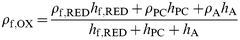 | (11) |
where the “ ρi" values denote the component densities (see above) and the “ hi" values denote the contributions to the total film thickness of the individual (subscripted) species. The experimental data ( Fig. 11 and 12) provide ρf,OX, ρf,RED, hf,RED and ( hf,RED + hPC + hA) (= hf,OX). There are two unknowns, hPC and hA, in eqn. (11), so we need two pieces of information. In addition to eqn. (11), we can relate the masses of anion and polymer via the doping stoichiometry. Specifically, since the doping level is 0.35 [ eqn. (12)]:
 | (12) |
Using this in eqn. (11) yields hPC/ hf,RED = 0.48, i.e. complete oxidation of the fully reduced polymer results in solvent transfer that swells the film by 48%. The observed swelling, ( hPC + hA)/ hf,RED≈0.63 (see Fig. 12). Hence hA/ hf,RED ≈ 0.15, i.e. anion entry (to maintain electroneutrality) swells the film by 15%. Crudely, since each anion contains 7 “heavy" atoms, and is associated with 33 “heavy" atoms in the polymer (three monomer units each containing 11 “heavy" atoms), this is physically reasonable.
The responses of Fig. 11 and 12 show significant hysteresis, rather like those in the raw TSM responses ( Fig. 5–8), and certainly much greater than in Qvs.E plots ( Fig. 9). This leads us inexorably to the conclusion that the film viscoelastic characteristics (see Fig. 13 and 14, below) are governed not by charge variations per se, but rather by the dramatic solvation changes they engender. The hysteresis, in response to potential changes, of the various parameters is then a consequence of slow solvent transfer and/or polymer reconfiguration that facilitates it.
 | ||
| Fig. 13 Plots of fitted storage modulus, G′, as a function of potential (panel a) and charge density (panel b) for the data of Fig. 5 and its third, fifth and seventh harmonic analogs. Symbols as in Fig. 11. | ||

Effect of potential. Plots of shear modulus components as functions of applied potential for four harmonics are shown in Fig. 13 ( G′) and 14 ( G″). In panels a and b, respectively, the moduli are plotted against applied potential and the resultant injected anodic charge. No G″ data are shown at the fundamental frequency, since the values were too small to determine reliably ( G″/ G′ < 0.1; see above). We make four observations.
First, individual shear modulus components show hysteresis with respect to both potential and charge. This is more obvious pictorially for the higher frequency data, for which the shear moduli are larger, but the inset to Fig. 13 highlights that this is true for all the data obtained. We therefore conclude that, despite a little irreversibility (in a thermodynamic sense) of charge injection/removal, the shear moduli at a given potential, determined on the time scale of our measurements, reflect the immediate prior history of the film. Such history effects have been postulated and discussed previously in the context of mobile species transfers and polymer reconfigurational processes. 66 The film thickness and density data of Fig. 11 and 12 unequivocally indicate that solvent swelling/deswelling is far from equilibrium on the time scale of these measurements. Thus, the film shear moduli reflect not the film charge state per se, but rather the solvation state which it subsequently dictates. This is entirely plausible, since solvents act as “plasticisers" of polymeric materials. In the present context solvent transfers are extremely slow, most likely due to associated polymer reconfiguration processes with large activation barriers. We postulate that the ability of the system to achieve its “equilibrium" state at the extreme of the potential excursion—but not at intermediate values—may be due to the build-up of large electrostatic forces that trigger the reconfiguration.
Second, the oxidized (doped) polymer has significantly lower storage and loss moduli values than the reduced (undoped) polymer. This is a consequence of the entry of the solvent, which softens the film and “lubricates" the movement of the polymer chains past each other. The direction of solvent transfer, and thus of the change in shear modulus components, is readily explainable: the solvent is polar and is a better solvent for the charged ( cf. uncharged) polymer.
Third, the direction of the hysteresis in the shear modulus components mirrors that of the solvent transfers. During polymer oxidation the modulus values stay higher than one would anticipate their equilibrium values to be (based on charge). This is a consequence of the kinetic failure of solvent to enter the film and thus soften it. As one approaches the positive end of the potential excursion, one has a film whose charge state is largely “oxidized", but whose solvation state is still broadly that of the reduced polymer. Analogously, during polymer reduction the modulus values stay lower than one would anticipate their equilibrium values to be (based on charge). This is now a consequence of the kinetic failure of solvent to leave the film. Thus, as one approaches the negative end of the potential excursion, one has a film whose charge state is largely “reduced", but whose solvation state is still broadly that of the oxidized polymer.
Finally, the shear moduli are markedly frequency dependent. This leads to the second major objective of our study.
Effect of frequency. Qualitative inspection of Fig. 13 and 14 indicates that the shear moduli for PHT films in all oxidation/solvation states increase significantly with frequency, G″ more so than G′. This is consistent with a material in the transition region. 9 Our goal now is to quantify this behaviour.
Fig. 15 shows the shear modulus components for the reduced film ( E = 0 V) as a function of frequency, plotted on logarithmic axes. Since the plots appear broadly linear, we show least squares fits to an equation of the form log( G) = a + b log( f). For the G′ data we find b = 0.97 (±0.15) ( R = 0.95; n = 6) and for the G″ data we find b = 2.19 (±0.18) ( R = 0.99; n = 5). Although there is clearly scatter on the data and we only have one order of magnitude spread in the frequency regime, these data imply G′ ∝ ω and G″ ∝ ω2.
 | ||
| Fig. 15 Plots of log( G′) (□) and log( G″) (■) vs. log( f) for the fitted shear modulus components of Fig. 13 and 14 and their analogs at 90 and 110 MHz at E = 0 V. Lines represent least squares fits to the data (see text). | ||
Fig. 16 shows the corresponding plots for the oxidized film ( E = 0.9 V). The situation here is less straightforward. Specifically, the G′ data are non-monotonic with frequency, showing a maximum storage modulus at ca. 50 MHz, and the G″ values are not linear. (The lines drawn on the plot are not an attempt to fit the data, but rather lines of slope 1 and 2 for G′ and G″, respectively, to allow comparison with the behaviour of the reduced film.)
 | ||
| Fig. 16 Plots of (a) log( G′) (○) and (b) log( G″) (•) vs. log( f) for the fitted shear modulus components of Fig. 13 and 14 and their analogs at 90 and 110 MHz at E = 0.9 V. Dashed and full lines, respectively, are of slope 1 and 2 (see text). | ||
Discussion
Our long term goal is the manipulation of film shear moduli. En route to this, our immediate goal is to rationalize G( ω, E), i.e. the frequency and potential (charge) variations of the shear modulus. In general terms, despite a huge volume of literature (discussed elsewhere 7–9) on the viscoelastic characteristics of bulk polymers, there has been relatively little progress for thin films. Here we test the ability of the simple Voigt and Maxwell models, which have been widely used for bulk materials, to explain the functional variations of G′ and G″.We consider first the frequency variations of G′ and G″. Cursory comparison of Fig. 3a with the data of Fig. 13–16 shows that the Voigt model is inappropriate: it fails to predict any variation of G′ with ω. Qualitatively, the increasing values of G′ and G″ with frequency (see Fig. 13 and 14) are consistent with the Maxwell model ( Fig. 2b) in the rubbery regime (when ωτ < 1). Quantitatively, the power law variations ( Fig. 15 and 16) are not explained by the Maxwell model. We suggest that more sophisticated (multi-element) spring and dashpot models may be more successful, but do not pursue this since the increased number of fitting parameters would make uniqueness of fit an issue.
The variations of shear modulus components with potential are more complex and interesting. The experimental protocol involved measurements at fixed potentials, including a prior “hold" at the selected potential with the intent of allowing pre-equilibration before data acquisition. Thus, a film maintained at any given potential would be expected to have a unique composition and structure appropriate to that applied potential. Simplistically, one would then expect the shear modulus, at any specified frequency, to be single valued at any given potential. The fitted data ( Fig. 11–14) are clearly inconsistent with this view. That this is not a feature of the fitting procedures is clearly indicated by the presence of hysteresis in the raw data (see Fig. 5–8). We therefore now explore possible reasons for the observed hysteresis.
One possibility is that, despite similar globally averaged composition, the films may have spatial variations within them that reflect their prior history (here, direction of approach to a given potential). The quartz resonator is most sensitive to the state of the film nearest the electrode, so spatial variation of viscoelastic properties could lead to the hysteresis in the shear modulus responses to applied potential, as shown in Fig. 13a and 14a. Since the decay length for displacement in the film varies inversely with frequency (see above), the hysteresis from this source would increase with frequency, as we indeed observe. Such variations could pertain to the oxidation state (doping level) and/or the local solvent concentration. They might particularly be expected when a significant fraction of the film is in the reduced state (for which the conductivity is low) due to potential variations across the film.
A subsidiary question is how might such spatial variations arise? For “conducting" polymers, the electronic and ionic conductivities of the two redox states (doped and undoped) are very different. For different redox switching directions this leads to different conversion mechanisms, e.g. homogeneous throughout the film, from the inside outwards or from the outside inwards; this point has been explored for poly(3-methylthiophene) films. 67
The other possible causes of hysteresis we consider are associated with failure to establish equilibrium film composition on the time scale (minutes) of the experiment. Most obviously, this might be associated with slow charge transport or slow solvent transport. Note that these situations need not be associated with spatial compositional inhomogeneity (see above), i.e. we may have spatially uniform, but non-equilibrium, film ion and/or solvent populations.
In the case of slow ion transfer, the charge and shear modulus responses to potential would show equivalent hysteresis. Although there is some hysteresis in the Q vs.E plot ( Fig. 9), this effect is much less pronounced than in the G′ and G″ vs.E plots ( Fig. 13a and 14a). That failure to establish charge equilibrium is not the predominant cause of the shear modulus hysteresis is confirmed by the presence of hysteresis in the G′ and G″ vs.Q plots ( Fig. 13b and 14b).
In the case of slow solvent transfer, the hysteresis in G′ and G″ vs.E plots would greatly exceed that in Qvs.E plots; this is equivalent to saying that there would be substantial hysteresis in G′ and G″ vs.Q plots. This is exactly what we find ( Fig. 13b and 14b), indicating that solvent equilibration between the film and the solution is slow on the experimental time scale. It is interesting to note that the film density and thickness data ( Fig. 11 and 12), which were acquired sequentially for the different harmonics, show no temporal “drift". Thus, we conclude that the film solvent population at each potential is not changing significantly on the time scale of our measurements. One could postulate various models for the rate of solvent transfer, and use the time dependence of shear modulus variation as a measure of solvent transfer in order to determine the appropriate rate parameter; such investigations would involve much longer time scale observations than used here.
One interesting supplementary question is the origin of the maxima in the shear modulus values at partial redox conversion. We speculate that this may be due to the interplay of two opposing effects that increase, but in a functionally different manner, upon film oxidation: electrostatic stiffening and solvent plasticization. At low doping levels, we suggest that the former predominates, since there is insufficient driving force to cause significant solvent entry. At higher doping levels, we suggest that there is sufficient driving force for solvent entry for the latter to predominate.
There has been one study reported on the “electroplastic behaviour" of PHT, 68 in which values of G′ ≈ 8 × 10 9 dyn cm −2 and G″ ≈ 6 × 10 8 dyn cm −2 (based on tan δ ≈ 0.07) were found. However, the material used in that study was very different to ours. First, the “films" were sufficiently thick ( ca. 0.1 mm) to be considered as bulk material, whereas we have studied thin (< 1 µm) films. Second, most of the samples studied by Shiga et al. were of chemically ( cf. electrochemically) prepared polymer. Third, their technique used free-standing films exposed to air, not solvent. Consequently, their polymers had G values indicative of “glassy" materials, whereas our films have G values indicative of viscoelastic materials. Fourth, the simple mechanical nature of their measurements meant that the frequency range studied was 0.1–100 Hz, i.e. many orders of magnitude lower than in our study. Furthermore, the in situ nature of our study has allowed the effect of polymer charge state to be studied in a systematic manner.
Finally, we make some general observations on the variations of shear modulus we have determined. Our data indicate that PHT films exposed to propylene carbonate solutions are viscoelastic and rather lossy. The primary effect of oxidation is to cause the entry of solvent, which plasticizes the film; however there are kinetic limitations associated with solvent transfer. This situation can be qualitatively visualized using the scheme-of-squares type model illustrated in Fig. 17. This type of model has been used to describe slow redox driven solvent transfer in rigid electroactive polymer films at TSM resonators; there the principal manifestations were in the gravimetric response, optimally demonstrated through hysteresis in Δ Mvs.Q plots. Here, the underlying mobile species transfers are identical, but the principal manifestations of slow solvent transfer are in the viscoelastic response, which we demonstrate through hysteresis in Gvs.Q plots.
 | ||
| Fig. 17 Scheme-of-squares model for PHT in two oxidation states (indicated by superscripts “0" and “+"), each of which may exist in a solvated form (PHT 0S and PHT +S) and an unsolvated form (PHT 0 and PHT +). Redox state changes (doping/undoping) are represented by “horizontal" translations and solvation state changes are represented by “vertical" translations in the diagram. | ||
Conclusions
Quartz crystal impedance measurements are a rich source of information on electroactive polymer film rheological properties, parameterized through shear moduli. Thin films of poly(3-hexylthiophene) (PHT) exposed to propylene carbonate electrolyte solutions are viscoelastic at 25°C, and show film mechanical resonance effects. The storage and loss moduli vary significantly with applied potential and operating frequency (in the range 10–110 MHz). The p-doped film is substantially softer than the undoped film, and
G′ and
G″ variations with potential can show maxima at partial p-doping. Both storage and loss moduli for undoped PHT films increase monotonically with frequency in the range studied, but for doped PHT films the storage modulus goes through a maximum at
ca. 50 MHz under the conditions employed. A Voigt model is qualitatively incompatible with these observations, and a Maxwell model can qualitatively explain some features.
Even in fixed potential—nominally “equilibrium"—experiments there is dramatic hysteresis in shear modulus values determined during stepwise doping and undoping. From the G–Q– E relationship, we deduce that this is a consequence of extremely slow solvent transfer between the film and the solution phase. Qualitatively, this can be modeled using a scheme-of-squares representation involving doped and undoped PHT, both in solvated and unsolvated forms, in which redox transformations (coupled electron/ion transfer) are much faster than the associated solvation changes (solvent transfer). These non-equilibrium solvation states may or may not be associated with spatial compositional heterogeneity.
On the basis of the data obtained we suggest that appropriate selection of operating frequency, applied potential and time scale offer the prospect of manipulating film viscoelastic parameters in a controllable manner over several orders of magnitude, from “rubbery" to near “glassy" behaviour.
Acknowledgements
We thank the EPSRC for financial support, including a studentship for MJB.References
- J. F. Rusling and S. L. Suib, Adv. Mater., 1994, 6, 922 CrossRef CAS.
- R. J. Gale, Spectroelectrochemistry, Plenum Press, New York, 1988. Search PubMed.
- P. A. Christensen and A. Hamnett, Techniques and Mechanisms in Electrochemistry, Blackie, Glasgow, 1994. Search PubMed.
- Handbook of Surface Imaging and Visualization, ed. A. T. Hubbard, CRC Press, Boca Raton, 1995. Search PubMed.
- A. R. Hillman, in Electrochemical Technology of Polymers, ed. R. Linford, Elsevier Applied Science Publishers, London, 1987, p. 103, 241. Search PubMed.
- R. W. Murray, Molecular design of electrode surfaces, Wiley, New York, 1992. Search PubMed.
- J. D. Ferry, Viscoelastic Properties of Polymers, Wiley, New York, 1961. Search PubMed.
- J. J. Aklonis and W. J. MacKnight, Introduction to Polymer Viscoelasticity, Wiley, New York, 1983. Search PubMed.
- W. W. Graessley, Faraday Symp. Chem. Soc., 1983, 18, 7 RSC.
- Handbook of Conducting Polymers, ed. T. A. Skotheim, Marcel Dekker, New York, 1986. Search PubMed.
- J. Roncali, Chem. Rev., 1992, 92, 711 CrossRef CAS.
- P. Novák, K. Müller, K. S. V. Santhanam and O. Haas, Chem. Rev., 1997, 97, 207 CrossRef CAS.
- F. Garnier, G. Horowicz, X. Peng and D. Fichou, Adv. Mater., 1990, 2, 592 CrossRef CAS.
- D. Ofer, R. M. Crooks and M. S. Wrighton, J. Am. Chem. Soc., 1990, 112, 7869 CrossRef CAS.
- T. Kobayashi, H. Yoneyama and H. Tamura, J. Electroanal. Chem., 1984, 161, 419 CrossRef CAS.
- R. J. Mortimer, Chem. Soc. Rev., 1997, 26, 147 RSC.
- A. R. Hillman and E. F. Mallen, J. Electroanal. Chem., 1987, 220, 351 CrossRef CAS.
- A. Hamnett and A. R. Hillman, J. Electrochem. Soc., 1988, 135, 2517 CAS.
- A. R. Hillman and E. F. Mallen, J. Electroanal. Chem., 1988, 243, 403 CrossRef CAS.
- P. A. Christensen, A. Hamnett, A. R. Hillman, M. J. Swann and S. J. Higgins, J. Chem. Soc., Faraday Trans., 1992, 88, 595 RSC.
- A. R. Hillman, D. C. Loveday, D. E. Moffatt and J. Maher, J. Chem. Soc., Faraday Trans., 1992, 88, 3383 RSC.
- A. R. Hillman, M. J. Swann and S. Bruckenstein, J. Phys. Chem., 1991, 95, 3271 CrossRef CAS.
- S. M. Dale, A. Glidle and A. R. Hillman, J. Mater. Chem., 1992, 2, 99 RSC.
- A. R. Hillman and E. F. Mallen, J. Electroanal. Chem., 1990, 281, 109 CrossRef CAS.
- A. R. Hillman and E. F. Mallen, Electrochim. Acta, 1992, 37, 1887 CrossRef CAS.
- J. Penfold, R. M. Richardson, A. Zarbakhsh, J. R. P. Webster, D. G. Bucknall, A. R. Rennie, R. A. L. Jones, T. Cosgrove, R. K. Thomas, J. S. Higgins, P. D. I. Fletcher, E. Dickinson, S. J. Roser, I. A. McLure, A. R. Hillman, R. W. Richards, E. J. Staples, A. N. Burgess, E. A. Simister and J. W. White, J. Chem. Soc., Faraday Trans., 1997, 93, 3899 RSC.
- A. R. Hillman, A. Glidle, R. M. Richardson, S. J. Roser, P. M. Saville, M. J. Swann and J. R. P. Webster, J. Am. Chem. Soc., 1998, 120, 12882 CrossRef CAS.
- D. A. Buttry, in Electroanalytical Chemistry, vol. 17, ed. A. J. Bard, Marcel Dekker, New York, 1991, p. 1. Search PubMed.
- S. Bruckenstein and A. R. Hillman, in Handbook of Surface Imaging and Visualization, ed. A. T. Hubbard, CRC Press, Boca Raton, U.S.A., 1995, p. 101. Search PubMed.
- Acoustic Wave Sensors: Theory, Design, and Physicochemical Applications, eds. D. S. Ballantine, R. M. White, S. J. Martin, A. J. Ricco, E. T. Zellers, G. C. Frye and H.Wohltjen, Academic Press, NY, 1997. Search PubMed.
- V. E. Granstaff and S. J. Martin, J. Appl. Phys., 1994, 75, 1319 CrossRef CAS.
- H. L. Bandey, S. J. Martin, R. W. Cernosek and A. R. Hillman, Anal. Chem., in the press. Search PubMed.
- G. Z. Sauerbrey, Z. Phys., 1959, 155, 206 Search PubMed.
- “Applications of piezoelectric quartz crystal microbalances" in Methods and Phenomena, vol. 7, eds. C. Lu and A. W. Czanderna, Elsevier, Amsterdam, 1984. Search PubMed.
- K. K. Kanazawa and J. G. Gordon, Anal. Chem., 1985, 57, 1770 CrossRef CAS.
- S. Bruckenstein and M. Shay, Electrochim. Acta, 1985, 30, 1295 CrossRef CAS.
- S. J. Martin and G. C. Frye, IEEE Symp. Ser., 1991, 393 Search PubMed.
- A. Domack, O. Prucker, J. Rühe and D. Johannsmann, Phys. Rev. E, 1997, 56, 680 CrossRef CAS.
- A. R. Hillman, M. J. Brown and S. J. Martin, J. Am. Chem. Soc., 1998, 120, 12968 CrossRef CAS.
- R. Saraswathi, A. R. Hillman and S. J. Martin, J. Electroanal. Chem., 1999, 460, 267 CrossRef CAS.
- H. Muramatsu, X. Ye, M. Suda, T. Sakahura and T. Ataka, J. Electroanal. Chem., 1992, 322, 311 CrossRef CAS.
- P. A. Topart, M. A. M. Noël and H.-D. Liess, Thin Solid Films, 1994, 239, 196 CrossRef CAS.
- N. Oyama, T. Tatsuma and T. Takahashi, J. Phys. Chem., 1993, 97, 10504 CrossRef CAS.
- A. Glidle, A. R. Hillman and S. Bruckenstein, J. Electroanal. Chem., 1991, 318, 411 CrossRef CAS.
- P. A. Topart and M. A. M. Noël, Anal. Chem., 1994, 66, 2926 CrossRef CAS.
- H. Muramatsu, X. Ye and T. Ataka, J. Electroanal. Chem., 1993, 347, 247 CrossRef CAS.
- T. Okajima, H. Sakurai, N. Oyama, K. Tokuda and T. Ohsaka, Bull. Chem. Soc. Jpn., 1992, 65, 1884 CAS.
- C. Behling, R. Lucklum and P. Hauptmann, Meas. Sci. Technol., 1998, 9, 1886 CrossRef CAS.
- C. E. Reed, K. K. Kanazawa and J. H. Kaufman, J. Appl. Phys., 1990, 68, 1993 CrossRef CAS.
- R. Lucklum, C. Behling, R. W. Cernosek and S. J. Martin, J. Phys. D., 1997, 30, 346 Search PubMed.
- A. Domack and D. Johannsmann, J. Appl. Phys., 1996, 80, 2599 CrossRef CAS.
- O. Wolff, E. Seydel and D. Johannsmann, Faraday Discuss. Chem. Soc., 1997, 107, 91 RSC.
- R. Lucklum and P. Hauptmann, Faraday Discuss. Chem. Soc., 1997, 107, 123 RSC.
- S. J. Martin, V. E. Granstaff and G. C. Frye, Anal. Chem., 1991, 63, 2272 CrossRef CAS.
- D. Johannsmann, K. Mathauer, G. Wegner and W. Knoll, Phys. Rev. B, 1992, 46, 7808 CrossRef.
- N. Oyama, T. Tatsuma and K. Takahashi, J. Phys. Chem., 1993, 97, 10504 CrossRef CAS.
- H. L. Bandey, M. Gonsalves, A. R. Hillman, A. Glidle and S. Bruckenstein, J. Electroanal. Chem., 1996, 410, 219 CrossRef CAS.
- H. L. Bandey, A. R. Hillman, M. J. Brown and S. J. Martin, Faraday Discuss. Chem. Soc., 1997, 107, 105 RSC.
- T. Tatsuma, K. Saito and N. Oyama, J. Chem. Soc., Chem. Commun., 1994, 1853 RSC.
- T. Tatsuma, K. Saito and N. Oyama, Anal. Chem., 1994, 66, 1002 CrossRef CAS.
- E. J. Calvo, R. Etchenique, P. N. Bartlett, K. Singhal and C. Santamaria, Faraday Discuss. Chem. Soc., 1997, 107, 91 RSC.
- S. M. Reddy, L. P. Jones and T. J. Lewis, Faraday Discuss. Chem. Soc., 1997, 107, 177 RSC.
- M. Urbakh and L. Daikhin, Phys. Rev. B., 1994, 49, 4866 CrossRef CAS.
- R. Schumacher, Angew. Chem., Int. Ed. Engl., 1990, 29, 329 CrossRef.
- CRC Handbook of Chemistry and Physics, 56th edn., CRC Press, Cleveland, 1975, p. B-95. Search PubMed.
- A. R. Hillman and S. Bruckenstein, J. Chem. Soc., Faraday Trans., 1993, 89, 339 RSC.
- F. Chao and M. Costa, Synth. Met., 1990, 39, 97 CrossRef CAS.
- T. Shiga and A. Okada, J. Appl. Polym. Sci., 1996, 62, 903 CrossRef CAS.
Footnote |
| † Basis of a presentation given at Materials Chemistry Discussion No. 2, 13–15 September 1999, University of Nottingham, UK. |
| This journal is © The Royal Society of Chemistry 2000 |