Machine learning predicted inelasticity in defective two-dimensional transition metal dichalcogenides using SHAP analysis

Abstract

The manipulation of crystallographic defects in 2H-transition metal dichalcogenides (2H-TMDCs), whether pre- or post-synthesis, has garnered significant interest recently, as it holds the promise of tuning the thermal, chemical, and electronic properties of these materials. However, such desirable improvements often come at the cost of deteriorated elastic and inelastic properties, which may lead to serious concerns considering mechanical reliability issues. Therefore, persistent efforts are needed to explore the effects of energetically favorable vacancies on the mechanical properties of 2D TMDCs for an effective tuning of material properties for versatile applications. In this context, machine learning models trained on data based on molecular models can not only provide fast, efficient material models but also unearth crucial structure–property relations. However, such efforts are at an early stage of development. In this study, machine learning and deep learning techniques are used to analyze the mechanical properties of 2D transition metal dichalcogenides (TMDCs) in both pristine and defect forms. The goal is to predict failure stress, strain to failure, and strength based on chirality and strain. Various crystallographic defects were considered, and extensive molecular dynamics simulations were performed. XGBoost and densely connected neural network (DenseNet) algorithms were used to make accurate state-of-the-art predictions, and comparative evaluation and Shapley value analysis of both models are presented to improve interpretability.

---

1. Introduction

Two-dimensional transition metal dichalcogenides (2D TMDCs) have garnered significant interest due to their intriguing structural, electrical, magnetic, and mechanical characteristics.¹ For example, depending on their structural configuration and constituent elements, 2D TMDCs can behave as both semiconductors (H-VTe₂, H-ScS₂, T-NiS₂, T-CrO₂) and metals (T-CrS₂, T-NbS₂, H-NbS₂, H-NiS₂).^2,3 Crystallographic defects are often introduced in 2D TMDCs depending on the synthesis route. Alongside these inadvertently generated flaws, deliberate manipulation of growth parameters offers a method for intentionally promoting defect formation involving chalcogen atoms.⁴ Moreover, controlled creation of defects can be achieved by judiciously modulating process variables such as temperature, gas flow rates, precursor ratios, and the choice of substrate material, among other influential factors.^3,4

In 2D TMDCs, point imperfections can serve as sites for electronic scattering, leading to alterations in the band arrangement and bending.^3,5 Point defects can also cause recombination and restricted emission of photons. All of these phenomena are dependent on the unique electronic configuration of a particular imperfection. Interestingly, manipulating electrical properties in these materials through engineered chalcogen atomic defects can even lead to transitions from semiconducting to metallic behavior. Moreover, by intentionally creating chalcogen atomic defects on the outermost layer of 2D TMDCs, the generation of 2D magnets becomes feasible. For instance, introducing Se vacancies triggers the formation of Se-deficient line defects in VSe₂, unexpectedly resulting in room-temperature ferromagnetism.⁶ Additionally, tensile deformation has been demonstrated as a viable method to adjust the electronic properties (from semiconductor to metallic behavior) and magnetic characteristics (from anti-ferromagnetism to ferromagnetism) of 2D TMDCs. Similarly, compressive and tensile strains were shown to control spin polarization and exchange coupling, useful for applications in nano-switches.⁷ Furthermore, the engineered nanopores within materials like MoS₂ nanosheets play a crucial role in selectively allowing water molecules to pass while blocking salt ions, showcasing precise control over filtration performance and highlighting the biomimetic potential of nanotechnology to address global water scarcity challenges.⁸

2D TMDCs are inherently brittle, and defects can significantly deteriorate their performance, reducing their elastic moduli, strength, and toughness. For example, it was demonstrated that defects can not only impact the quasi-static strength of 2D TMDCs but also detrimentally influence their long-term performance, thus affecting reliability in device-level applications.⁹ Similarly, crystallographic defects were shown to significantly influence the fatigue strength of not only 2D TMDCs but 2D materials in general (such as graphene, graphene oxide, and 2D hybrid organic–inorganic perovskites).^10,11 Therefore, as 2D TMDCs are pushed toward more diverse and extreme applications with a host of functionalities, understanding the role of defects in their mechanical performance needs more careful attention and predictive modeling is desired.⁶ While density functional theory calculations of mechanical properties are very accurate, these computations incur significant computational expenses and are limited to pristine materials at absolute zero temperatures. Alternatively, although ab initio molecular dynamics simulations enable probing materials at finite temperatures, such endeavors are prohibitively costly, and there are only a handful of such attempts for forecasting the mechanical properties of pristine 2D materials. In this context, classical molecular dynamics calculations¹² emerge as a cost-effective alternative, enabling comprehensive parametric analysis encompassing factors like temperature and the strain rate on failure stress, failure strain, and toughness. Furthermore, these calculations also furnish unparalleled insights into the intricate mechanisms underpinning failure within atomically thin materials. However, thus far, these techniques have been employed to study the inelastic properties of 2D TMDCs on a case-by-case basis, which hinders efficient predictive modelling and optimization, especially at the fundamental level.

With remarkable progress in computational sciences, machine learning (ML) algorithms have enabled the development of ingenious strategies in materials design. ML models have also demonstrated their efficacy in predicting mechanical properties. By utilizing data from molecular dynamics (MD) simulations, deep learning algorithms can identify and understand the intrinsic connections between mechanical properties and various influencing factors. This, in turn, enables the prediction of crucial properties for desired materials. Notable efforts in this area include the prediction of the bulk moduli of metal–organic frameworks,¹³ nonlinear mechanical characteristics of cellular mechanical metamaterials,¹⁴ multi-scale constitutive elastic relations for nanoporous materials,¹⁵ microscale elastic strain field of three-dimensional (3D) high contrast elastic composites,¹⁶ prediction of dynamic crack propagation patterns in 3D solids, and mechanical property prediction of 3D spider webs.¹⁷ In the context of 2D material mechanics, however, only a limited number of attempts have been made to predict and employ ML so far. In their seminal work, Yang et al. employed graph neural networks to predict the effective tensile modulus of porous graphene.¹⁸ More recently, Jin et al. harnessed support vector machines to predict the mechanical properties of nickel–graphene nanocomposites.¹⁹ Xu et al. employed the extreme gradient boosting (XGBoost) algorithm to estimate the tensile strength of polycrystalline monolayer graphene oxide.²⁰ Also, Malakar et al. employed ML techniques to predict the fracture properties of cracked 2D Mo- and W-based chalcogenides.²¹ All these endeavors offer an efficient multi-scale approach, employing machine learning models on mechanical property data derived from atomistic modeling for the purpose of rational design of structures and devices.

In this study, we have employed machine learning and deep learning techniques to study the inelastic properties of pristine and defective 2D TMDCs. The objective is to predict chirality-dependent failure stress, strain to failure, and toughness for 2D TMDCs in their pristine and defective forms as a function of strain rate. The selection of these materials was motivated by the objective to encompass semiconducting, metallic, magnetic, and nonmagnetic systems with a diverse array of chalcogen elements exhibiting varying electronegativities, as well as transition metal elements characterized by a spectrum of unpaired d electrons. Several crystallographic point defects were taken into account, including an isolated vacancy of a transition metal atom (V_M), a lone chalcogen vacancy (V_C), double vacancies involving chalcogen elements (V_2C), and a defect comprising one transition metal atom along with two chalcogen vacancies (V_1M-2C). A comprehensive set of classical molecular dynamics (MD) simulations, totaling ∼666, were conducted at strain rates ranging from 10⁷ s⁻¹ to 10¹⁰ s⁻¹. Firstly, we employed the XGBoost²² algorithm due to its ability to handle complex relationships in data, effectively capture feature importance, and deliver accurate predictions for challenging structural integrity scenarios. Additionally, the densely connected neural network²³ algorithm was employed to improve the declined accuracy caused by the vanishing gradient in high-level neural networks. We provide a succinct comparative evaluation of DenseNet and XGBoost models, accompanied by a comprehensive summary of the entire model architecture and its key findings. Furthermore, we conducted a Shapley value analysis to elucidate the inner workings and interpretability of both DenseNet and XGBoost models.

2. Methodology

2.1. MD simulation method

The Large-scale Atomic/Molecular Massively Parallel Simulator (LAMMPS)²⁴ was employed to conduct classical molecular dynamics simulations for a total of 17 2D TMDCs; specifically, we considered 2H phases of CrO₂, CrS₂, CrSe₂, CrTe₂, NbS₂, NbSe₂, NiS₂, NiSe₂, NiTe₂, ScO₂, ScS₂, ScSe₂, ScTe₂, VO₂, VS₂, VSe₂, and VTe₂. The defect-free 2D TMDC samples comprised 9408 atoms with an area of 255 nm² in the X–Y plane. To ensure periodicity, boundary conditions were applied in all three orthogonal directions. To prevent unphysical interlayer interactions originating from periodic boundary conditions, a vacuum of 10.6 nm was added in the Z (out-of-plane) direction. The interatomic interactions for all the MX₂ (Sc-, Ni-, V-, Nb-, and Cr-based chalcogenides, i.e., O, S, Se, and Te) samples were modeled using the Stillinger–Weber potential parameterized for 2D TMDCs.² In the H-phase, four types of vacancies (V_M, V_C, V_2C, and V_1M-2C) were created by selectively removing atoms, as depicted in Fig. S1 (ESI†). For structural relaxation at 300 K, an isothermal–isobaric ensemble was utilized. The Nose–Hoover thermostat with a relaxation time of 0.1 ps was employed to maintain temperature, and the total simulation time for thermal equilibration at 300 K was set as 20 ps. The simulation timestep was chosen as 1 fs, a value consistent with previous studies. At the beginning of thermal relaxation, every atom was assigned a random velocity from a Gaussian distribution to accommodate for stochasticity arising from thermal fluctuations. To investigate the response of the material to uniaxial tensile forces, experiments were performed at five distinct strain rates, ranging from 10⁷ to 10¹⁰ s⁻¹, covering a wide range of values. To account for Poisson's effect, the simulation cell was uniaxially expanded, keeping the length in the perpendicular in-plane direction unconstrained. The virial stresses acting on individual atoms were calculated and averaged for every time step.

2.2. Data processing

ML-Based pre-processing of raw MD data from 666 independent MD calculations for cleaning, mining, and extraction of 9 different features were implemented. These features include ‘strain,’ ‘metal atomic mass,’ ‘chalcogen atomic mass,’ ‘strain rate,’ ‘defect type,’ ‘defect size,’ ‘electronegativity difference,’ ‘chirality,’ and ‘number of unpaired electrons.’ The ‘number of unpaired electrons’ is determined using the stable electronic configuration of the transition metals (data regarding the ‘number of unpaired electrons’ are obtained from the Royal Society of Chemistry's website²⁵). The label encoding of chirality was done by assigning ‘Armchair’ as 0 and ‘Zigzag’ as 1. A summary of all the input features is presented in Table 1. Furthermore, the entire dataset was organized in the Pandas²⁶ DataFrame format to serve as input for the machine learning model pipelines. In addition to DenseNet^23,27 and XGBoost algorithms, a model based on a feedforward neural network (FFNN)²⁸ was also developed to understand behavior at isolated points, without any ensemble or hidden layer temporal connections, relying solely on material properties and strain values. Details regarding FFNN methodology are provided in the ESI.† To ensure uniformity and comparability among the features, the dataset underwent z-score normalization,²⁹ which scales the features to have a mean of zero and a standard deviation of one. This process minimizes the influence of different feature ranges, ensuring that features with larger numerical values do not dominate the learning process due to their magnitudes.

Table 1 Description of some input features of the FFNN and DenseNet model. Atomic mass values for the transition metals and chalcogen atoms are given in atomic units. Electronegativity values are taken from the Royal Society Chemistry website²⁵

Features	Values
Metal atomic mass	Sc (44.96), Ni (58.69), V (50.94), Cr (51.99), Nb (92.90)
Chalcogen atomic mass	O (16.00), S (32.06), Se (78.96), Te (127.6)
Chiral directions	Armchair, zigzag
Strain rates (s^−1)	10^10, 10^9, 10^8, 10^7
Defects types	Pristine, VM, VC, V2C, V1M-2C
Number of unpaired electrons	Sc (1), Ni (2), V (3), Cr (6), Nb (5)
Electronegativity values of metals and chalcogens	Sc (1.36), Ni (1.91), V (1.63), Cr (1.66), Nb (1.6), O (3.44), S (2.58), Se (2.55), Te (2.1)

---

2.3. The XGBoost model

XGBoost, an abbreviation for extreme gradient boosting, represents a machine learning algorithm that belongs to the ensemble learning paradigm. XGBRegressor, a variant of XGBoost tailored for predictive modelling of continuous numerical values, was employed particularly for our task of predicting stress, failure stress, and failure strain. The parameterization of the model is structured as follows: the ‘booster’ is designated as ‘gbtree’, ‘device’ is allocated to ‘cpu’, ‘validate-parameters’ is explicitly set to ‘False’, ‘eta’ assumes a value of 0.3, ‘gamma’ is configured as 0.0, ‘max-depth’ is defined as 6, ‘min-child-weight’ is stipulated at 1, ‘max-delta-step’ is specified as 0, ‘sub-sample’ is established as 1, ‘sampling-method’ is selected as ‘uniform’, ‘max-leaves’ assumes a value of 1, ‘max-bin’ is set to 256, and ‘num-parallel-tree’ is configured to 1, with the remaining hyperparameters retaining default values.

2.4. The DenseNet model

In this study, a numerical optimization technique is employed to determine the optimal structure of the hidden layer within a neural network (NN). The search for the optimal NN structure entails globally tracking across the entire accessible parameter space. In this context, the accessible parameter space is defined by the best parameters, which vary in terms of the number of hidden layers and neurons within each layer. This broad search space is deliberately chosen to ensure the discovery of the most suitable NN architecture for the specific application. The hyperparameters of the NN model are listed in Fig. 1(a). By conducting this global search for the optimal NN architecture, the research aims to identify the configuration that leads to the most accurate stress–strain curve predictions for 2D TMDCs based on the provided dataset and input features. This DenseNet model employs the backpropagation algorithm³⁰ to calculate the derivatives of the error function concerning the hidden layer weights and biases. Batch gradient descent methods are utilized to minimize the error functions. Specifically, the batch gradient method computes the gradient of the entire dataset for each iteration, helping to update the model parameters more efficiently.³¹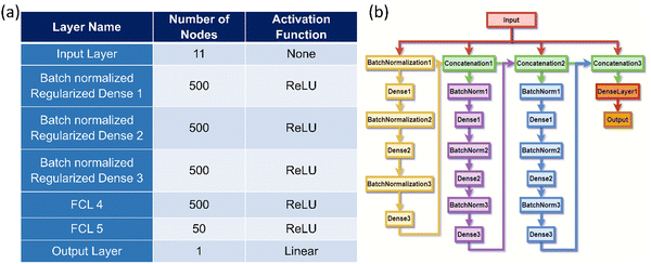

Fig. 1 (a) Details regarding the DenseNet model architecture. (b) Schematic representation of the DenseNet model.

As shown in Fig. 1(b), the DenseNet model was developed with three building blocks connected in succession. Each block consists of three consecutive batch normalized and regularized dense layers,³² where the output of each block is concatenated with the input layer and concatenated layer of the previous block's output to form the input of the next block. In this way, the last block contains all the blocks and layers previously used as input for the model. A single block unit is composed of one linear (Dense) unit with ‘ReLU’ activation,³³ a kernel initializer, and a kernel L2 regularizer³⁴ of 0.01. L2 regularization was applied to the model during the training process to mitigate overfitting. This regularization technique enhances the generalization ability of the model and prevents it from excessively memorizing the training data. Furthermore, as an optimizer in this study, Adam³⁵ is employed. Adam is a stochastic gradient descent method that performs adaptive estimation of the 1st and 2nd order moments of the gradients. By leveraging Adam, the convergence of the model during training is enhanced, and it aids in finding better optima in the parameter space for improved performance in stress–strain curve prediction for 2D TMDCs.

2.5. Shapley additive explanation

Shapley additive explanation, or SHAP,³⁶ is a game-theoretic approach used to explain or interpret the output of a machine learning model. It leverages classical game theory, employing Shapley values to combine both local and global feature dependency models into an additive framework. By employing Shapley modelling, the behavior of the model output can be elucidated for all 9 features in our dataset through various feature combinations and experimentation techniques, all with straightforward implementations. Bar plots and beeswarm plots were utilized to illustrate the variations in output values (such as how failure stress and toughness change with different feature values) with manipulation of the features.

One of the main objectives of this research was to determine how a single feature or multiple combinations of features actually change the output of a model. A game-theoretic approach was employed to understand and interpret each feature by systematically combining it with the remaining 8 features. For each feature, it was excluded from the feature set first, and various combinations or elements from the superset of features were considered, averaging over the results. These averages were then compared with the expected output of the model with all 9 features combined. The mathematical model of Shapley can be represented with the impact on model output with Shapley values given by where S is all the subsets of the feature excluding feature i from the feature space. The difference of expectations of outputs of these feature spaces can be calculated as Shapley values to quantify the ‘impact on model output’ parameter. M is all the 9 features together as a set. Here, f_x implies the expected values. The Shapley values were calculated on 5000 test data points for both DenseNet and XGBoost interpretability.

2.6. Error analysis and evaluation indicator

In our study, the ML and DenseNet deep learning methods employed a typical loss function, combining the mean squared error (MSE) function with an L2 regularization loss function given by where N represents the total number of sample points, y_pi denotes the predicted output for each set of samples, y_i stands for the actual target data, and α represents the L2 regularisation parameter. The first term in the loss function calculates the MSE between the predicted output and the actual target data. In contrast, the second term applies L2 regularisation to penalize the weights (W) to prevent overfitting and enhance model generalization.

The coefficient of determination (R²) was used to evaluate the performance of different models. R² is a statistical metric that indicates how well the predictions of the model fit the actual data. A higher R² value signifies a more accurate forecast. The R² is given by where Y represents the average of the target data across all samples. By comparing the R² values, we can assess the predictive performance of the model in stress–strain curve prediction for 2D TMDCs. The regularization parameter α plays a crucial role in controlling overfitting by penalizing large weights and promoting a more generalizable model.

3. Results

3.1. Insights from the data

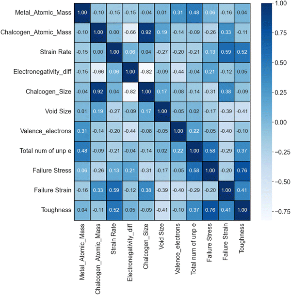
Out of a total of 666 samples, 102 (15%) were allocated to the test set, while the remainder constituted the training and validation sets. The training data points underwent random shuffling, treating each point as an independent random variable, while considering the stress value for a given strain value as the ’property of the material corresponding to the given inputs. The data were split into 90% for training and 10% for validation after shuffling (the dataset was split using the train_test_split method of the scikit-learn library, which has a built-in feature of random shuffling). Notably, analyzing the test dataset was ignored, treating it as an independent entity to assess the robustness of the model. By generating a heatmap³⁷ of Pearson's correlation values for the input features and output features (except stress), using the pandas DataFrame corr() method, as shown in Fig. 2, based on the training dataset, the correlation between the features and the target values was successfully visualized. This analysis provided valuable insights into the relationships (collinearity) of the variables and potential predictive capabilities. The heat map captures the impact of varying feature values on failure stress and toughness and provides a visual indication of the influence of factors such as void size and the number of unpaired electrons on failure stress, failure strain, and toughness. Notably, the heat map reveals a positive correlation between failure stress and the number of unpaired electrons, as well as a small positive correlation between failure stress and the strain rate, as well as electronegativity difference. This correlation indicates that an increase in the strain rate or the number of unpaired electrons corresponds to an increased stress response. A detailed explanation for these observations and the underlying governing mechanisms is provided in Section 4.1.

Fig. 2 Pearson's correlations between various input features and target variables (failure stress, failure strain, toughness). The number of unpaired electrons in transition metals has a significant impact on the mechanical properties.

A notable positive correlation between the number of unpaired electrons in transition metals and their valence electrons is observed. However, this trend does not extend to the relationship between valence electrons and mechanical properties such as failure stress and toughness. In these cases, valence electrons demonstrate a negligible and inverse correlation with both toughness and failure stress. Given these findings, analysis of this study is focused on the ‘number of unpaired electrons in transition metals’ as the primary feature of interest. The approach was strategically shifted, replacing the ‘number of valence electrons in transition metals’ with the ‘number of unpaired electrons in transition metals’ as the key variables. This alteration led to a significant improvement in the predictive accuracy of both the DenseNet and XGBoost models. The enhanced performance, along with the conclusive results and insights gained from the model analyses, affirm the effectiveness of this modification.

A substantial positive correlation exists between the chalcogen atomic mass and chalcogen size. Consequently, to avoid redundancy in the model, it was a more logical approach not to include both features in our trained models. The decision to exclude the chalcogen size as a feature is rooted in the recognition that highly correlated features can introduce redundancy and potentially lead to overfitting, undermining the interpretability and generalization capabilities of the model.

3.2. DenseNet model

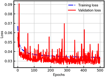
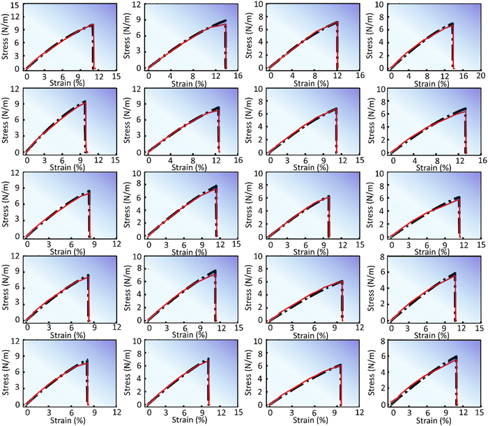
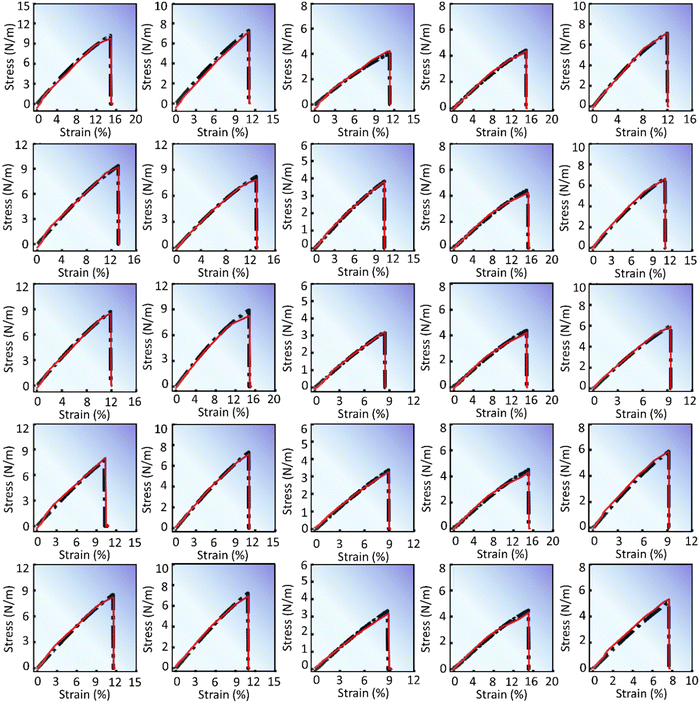
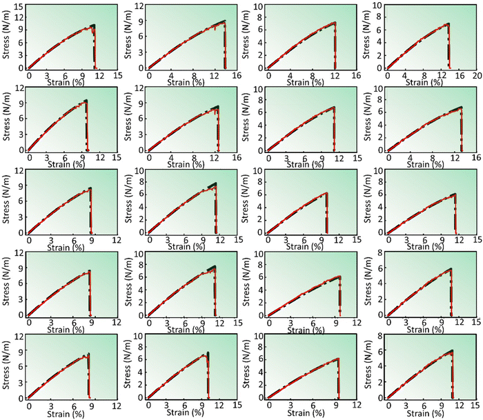
The DenseNet model was constructed using the Keras library with the TensorFlow framework³⁸ at the backend. The model underwent an extensive training regimen spanning 500 epochs, during which EarlyStopping³⁹ callbacks with the patience parameter set to 200 were implemented. Notably, the training process continued until the 500th epoch, and the best model within this epoch range was saved. Throughout the training journey, the model consistently demonstrated a decreasing trend in loss for both the training and validation datasets, as depicted in Fig. 3. While sporadic high peaks in the validation loss curve were observed, the overarching trend showcased a declining loss, with such peaks indicating potential instances of overfitting. This sustained reduction in loss over the training period underscores the effectiveness and reliability of our DenseNet model as a proficient predictive tool, a conclusion further substantiated by the stress–strain curve visualizations.

Fig. 3 Loss in the training process of the DenseNet model.

The predictions generated by the DenseNet model are presented in Fig. 4 and 5. These figures display stress–strain curves, contrasting the predicted (red curve) and actual (black curve) behaviors. Each set of plots, characterized by distinct subfigures, corresponds to specific pattern types and trends as described in their respective figure captions. Fig. 4 presents the stress–strain response of pristine and defective (pristine, V_2C, V_C, V_M, and V_1M-2C, from top to bottom) V-based 2D TMDCs with different chalcogen elements (O, S, Se, and Te, from left to right) for a strain rate of 10⁸ s⁻¹ along the armchair direction. Similarly, Fig. 5 presents the stress–strain response of pristine and defective (V_2C, V_C, V_M, and V_1M-2C, from top to bottom) Se-based 2D TMDCs containing Cr, Nb, Ni, Sc, and V (from left to right) as the transition metal, for a strain rate of 10⁷ s⁻¹ along the armchair direction. Upon meticulous examination of Fig. 4 and 5, an interesting observation emerges: the overall predicted stress–strain curves across all subfigures within Fig. 4 and 5 closely mirror the corresponding actual stress–strain curves. This consistent alignment underscores the robust predictive capability of the DenseNet model. However, subtle deviations emerge near the point of failure. Notably, these discrepancies are particularly noticeable at the failure point, and minor deviations are discernible in the mid-section of the stress–strain curve. Moreover, Fig. S2 (ESI†) presents the stress–strain predictions for various pristine samples, considering both chiral orientations (armchair and zigzag) and incremental strain rates.

Fig. 4 DenseNet model predictions to capture the variation for different chalcogens O, S, Se, and Te (left to right) along with varying defects pristine, V_2C, V_C, V_M, and V_1M-2C (top to bottom). The transition metal and strain rate are fixed as vanadium (V) and 10⁸ s⁻¹, respectively. All the subfigures present stress–strain responses in the armchair direction.

Fig. 5 DenseNet model predictions to capture the variation for different metals Cr, Nb, Ni, Sc, and V (left to right) along with varying defects pristine, V_2C, V_C, V_M, and V_1M-2C (top to bottom). The chalcogen and strain rate are fixed as Se and 10⁷ s⁻¹, respectively. All the subfigures present stress–strain responses in the armchair direction.

In the course of the hyperparameter tuning process, attention was directed towards several deep learning hyperparameters, including the activation function, batch size, and learning rate. The selection of optimal hyperparameters was guided by assessing the performance of the model on the validation set, which served as a pivotal evaluation metric. The approach of this study involved a systematic exploration of various combinations of these hyperparameters, with the primary objective being the identification of a configuration that not only maximized the performance of the model but also yielded the most favorable results. Fig. 6 displays scatter plots depicting the relationship between predicted and actual values for failure stress, failure strain, and toughness. Notably, these scatter plots are exclusively generated for the test set, and the predictions are quite good, with a highest R² of 0.98 in the case of failure stress. However, in Fig. 6, certain data points, particularly evident in the scatter plot correlating failure stress and toughness, exhibit notable deviations from the overarching linear trend.

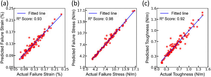Fig. 6 Scatter plots of predicted (using DenseNet) and actual values for (a) failure strain, (b) failure stress, and (c) toughness.

Additionally, the DenseNet model yielded a favorable R² score of 0.98, 0.98, and 0.95 on the training, validation, and testing sets, respectively, indicating its strong predictive capabilities. The R² scores for DenseNet, incorporating the valence electrons of the transition metal as a feature in lieu of the number of unpaired electrons of the transition metal, are 0.97, 0.97, and 0.95 for the training, validation, and testing sets, respectively. Despite the comparability of R² scores, it is noteworthy that, in terms of performance, the predictions were not as satisfactory as those achieved with the inclusion of the number of unpaired electrons of the transition metal.

3.3. Machine learning models

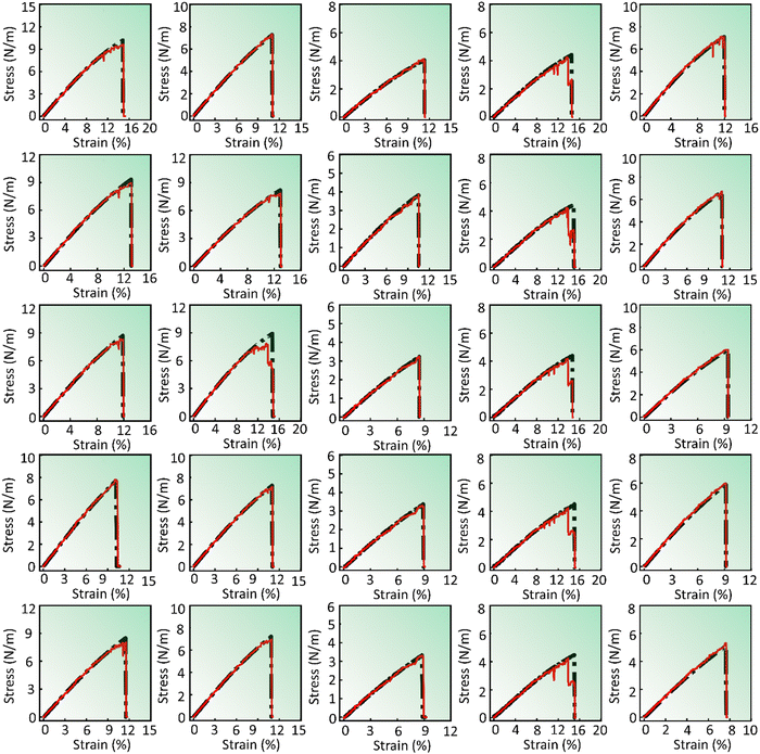
In our machine learning framework, the XGBoost model has been implemented successfully. The predictions made by XGBoost have proven to be of exceptional accuracy, and notably its training time is significantly lower than that of DenseNet while still delivering remarkable predictions. For details regarding training time requirements, please check out Section 4.2.

The predictions generated by the XGBoost model are presented in Fig. 7 and 8. Fig. 7 presents the stress–strain response generated by XGBoost for pristine and defective (pristine, V_2C, V_C, V_M, and V_1M-2C, from top to bottom) V-based 2D TMDCs with different chalcogen elements (O, S, Se, and Te, from left to right) for a strain rate of 10⁸ s⁻¹ along the armchair direction. Similarly, Fig. 8 presents the stress–strain response of pristine and defective (V_2C, V_C, V_M, and V_1M-2C, from top to bottom) Se-based 2D TMDCs containing Cr, Nb, Ni, Sc, and V (from left to right) as the transition metal, for a strain rate of 10⁷ s⁻¹ along the armchair direction. Furthermore, the stress–strain predictions for a range of pristine samples are shown in Fig. S3 (ESI†), which takes into account incremental strain rates as well as chiral orientations (zigzag and armchair).

Fig. 7 XGBoost model prediction to capture the variation for different chalcogens O, S, Se, and Te (left to right) along with varying defects pristine, V_2C, V_C, V_M, and V_1M-2C (top to bottom). The transition metal and strain rate are fixed as vanadium (V) and 10⁸ s⁻¹, respectively. All the subfigures present stress–strain responses in the armchair direction.

Fig. 8 XGBoost model prediction to capture the variation for different metals Cr, Nb, Ni, Sc, and V (left to right) along with varying defects pristine, V_2C, V_C, V_M, and V_1M-2C (top to bottom). The chalcogen and strain rate are fixed as Se and 10⁷ s⁻¹, respectively. All the subfigures present stress–strain responses in the armchair direction.

The stress–strain curves generated by the XGBoost model exhibit noticeable deviations from the actual curves, particularly in the vicinity of the near-failure point, similar to DenseNet predictions. The discrepancies are evident when comparing the stress–strain curves depicted in Fig. 8, where the model falls short of accurately capturing the behavior, as indicated by the superior performance of the DenseNet predictions illustrated in Fig. 5. Further examination reveals that the stress–strain curves in Fig. 7 exhibit a relatively improved correspondence with the actual data, surpassing the predictive capabilities demonstrated in Fig. 8. However, challenges persist, particularly in Fig. 8, where the XGBoost model encounters difficulties in fully capturing the nuances of the near-failure point. This discrepancy is evident as the model fails to accurately replicate the actual stress–strain path shown in the figures.

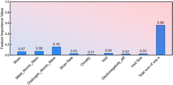
These observations suggest a need for refinement or adjustment in the XGBoost model, particularly in its capacity to precisely model the near-failure region of stress–strain curves. Addressing this issue may contribute to a more accurate representation of the material behavior, aligning the predictions of the model more closely with the actual data. As shown in Fig. 9, the feature importance plot highlights the significance of the number of unpaired electrons of the transition metal as a crucial feature for prediction. This observation emphasizes the relevance of electron configuration in influencing the material properties under consideration, substantiating its importance in the predictive capabilities of the XGBoost model.

Fig. 9 Feature importance determined by the XGBoost model.

Additionally, Fig. 10 presents scatter plots that illustrate the correlation between predicted and actual values for failure stress, failure strain, and toughness. Notably, the R² values associated with these scatter plots do not surpass the R² values exhibited in the scatter plots generated for DenseNet (refer to Fig. 6). This indicates a comparative performance lag in the predictive capabilities of the XGBoost model. The observed discrepancy in R² values suggests that, in the context of failure stress, failure strain, and toughness predictions, the XGBoost model may not be performing as effectively as the DenseNet model. Further analysis and potential adjustments to the XGBoost model may be necessary to enhance its predictive accuracy in capturing the intricate relationships between input features and the material properties of interest.

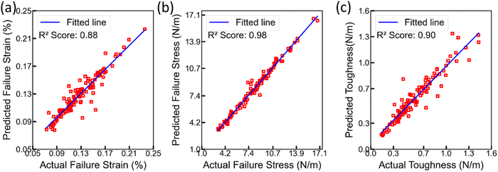Fig. 10 Scatter plots of predicted (using XGBoost) and actual values for (a) failure strain, (b) failure stress, and (c) toughness.

However, the XGBoost model produced exceptional R² scores of 0.99 on the training set and 0.99 on the development set. Furthermore, an R² score of approximately 0.93 was achieved on the test set. The stress–strain and scatter plots have been exclusively generated for the test set, and the outcomes demonstrate exceptional performance in terms of R² score. The presence of serrations near the point of failure in the stress–strain plots generated by XGBoost can be attributed to the limitation of the model in accurately capturing the abrupt failure, which leads to the observed irregularities in the plots. However, the overall results attained from the evaluation of the unseen test set reveal the impressive accuracy and efficacy of the XGBoost model in predicting the aforementioned parameters.

4. Discussion

4.1. Interpretable machine learning

The aforementioned models, namely XGBoost and DenseNet, operate as ‘black box’ models because of the opacity of their decision-making and output-generating procedures. It would be helpful to improve our comprehension of these models by clarifying how they behave locally and globally across particular datasets. Understanding the characteristics of a model and how they affect the desired output values in the context of classification or regression problems is essential to making sense of them. Here, the SHAP framework was used to unearth explanations of the overall dataset and particular data point instances, respectively. The Shapley method was utilized to assess overall feature dependence and to comprehend the variability and distribution of impact values, with the beeswarm plot employed for visualizing these distributions. To understand the model decision logic and achieve interpretability, the influence of each input feature on the outcome of model predictions was quantified by computing the Shapley values corresponding to each input feature and its variances.

Fig. 11 presents the box plots of the mean Shapley values for the XGBoost and DenseNet models. These plots illustrate the absolute impact of 9 feature metrics on the model output, providing a clear depiction of the intensity of the impact of each feature. 5000 data points for both XGBoost and DenseNet from the test data were utilized to gain inherent model interpretability, demonstrating that, with the same dataset from the test set, DenseNet can extract valuable insights and prove more robust for predicting test results compared to the XGBoost model. Fig. 11 displays the impact values of DenseNet and XGBoost, where both models exhibit distinct orders of absolute impact values for all features.

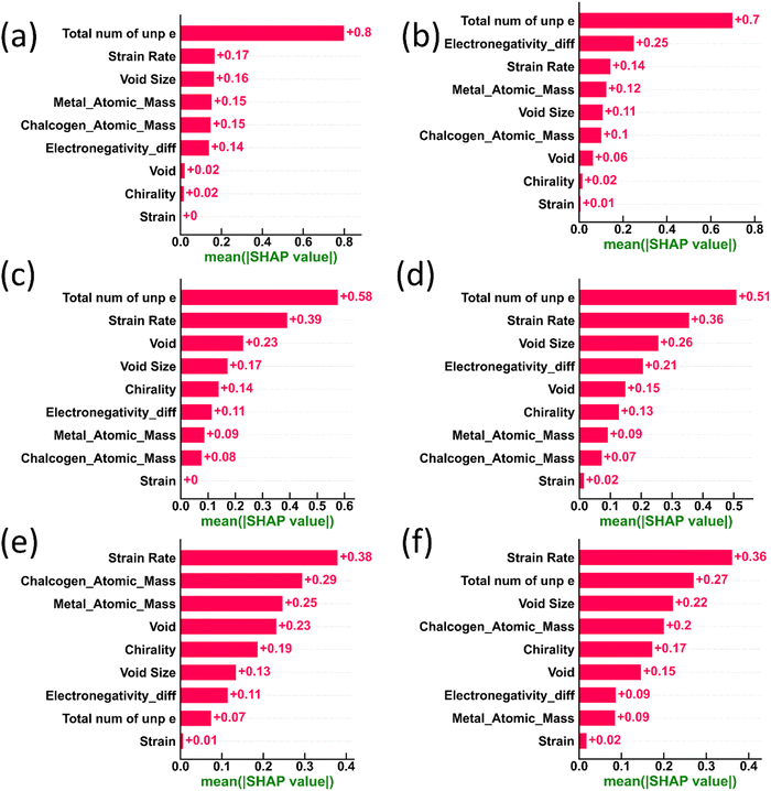Fig. 11 The impact of features on both XGBoost and DenseNet outputs for (a) and (b) failure stress, (c) and (d) toughness, and (e) and (f) failure strain, respectively.

In the realm of transition metal dichalcogenides (TMDCs), the intrinsic bond strength is significantly contingent upon the charge transfer characteristics between the constituent chalcogen and transition metal atoms.^40,41 Empirical evidence suggests a diminution in charge density from sulfides to tellurides, implying a gradual weakening of covalent bonds within the basal plane.⁴² This phenomenon underscores the pivotal role of charge transfer in modulating bond robustness, corroborated by the correlation between bond strength and the electronic configuration, specifically the number of unpaired electrons in the atomic structure.

Additionally, a larger difference in electronegativity between two bonding atoms typically makes the bond stronger, as it tends to be more ionic. This implies that 2D sulfides should be stronger than selenides and tellurides. For example, as shown in Fig. 4 and Fig. S4 (ESI†), in terms of strength, VS₂ > VSe₂ > VTe₂ and CrS₂ are stronger than CrSe₂ and CrTe₂. This conclusion is in agreement with previous reports on pristine 2D TMDCs wherein an identical trend was observed for elastic constants and microhardness.^43,44 This same trend remains intact for samples with isolated defects as well. Future explorations should look into the effect of interacting defects.

The beeswarm plots shown in Fig. 12 provide a visual representation of all the Shapley values, with the Y-axis organizing values based on features. Each group on the Y-axis is color-coded according to feature values, with higher feature values appearing in a redder hue. These plots facilitate the comprehension of inter-feature relationships. In the XGBoost model, for instance, in the case of the number of unpaired electrons in transition metals, an increase in feature values corresponds to a rise in the Shapley value (see Fig. 12(a), (c) and (e)). This implies that higher values of unpaired electrons are associated with increased material failure stress and toughness. Conversely, materials with fewer unpaired electrons are predicted to have lower toughness in TMDCs, aligning with the previously reported impact of charge transfer. Similarly, the strain rate exhibits a positive association with failure stress, strain, and toughness, suggesting enhanced mechanical properties at higher deformation rates.

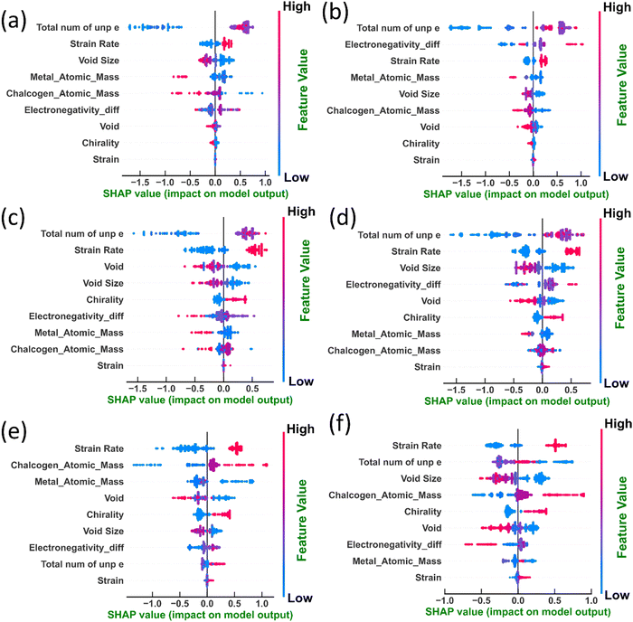Fig. 12 The impact of features on both XGBoost and DenseNet outputs for (a) and (b) failure stress, (c) and (d) toughness, and (e) and (f) failure strain, respectively.

In terms of void size concerning toughness, failure strain and failure stress values, a larger value corresponds to diminished material properties. This suggests that voids act as stress concentrators, promoting crack initiation and propagation, an observation in line with previous observations.^9,45,46 However, as shown in Fig. 11, the effect of void size is more pronounced on toughness and failure strain than on failure stress. Notably, the atomic mass of both metals and chalcogens also negatively impacts toughness, potentially due to its influence on material density and interatomic forces. Fig. 12(f) further reveals intriguing nuances in the ’behavior of the model concerning failure strain. Unlike toughness, the number of unpaired electrons exhibits a moderately negative influence on failure strain. This suggests a trade-off between intrinsic strength and ductility, where higher electron delocalization enhances strength but may reduce deformability. Interestingly, the strain rate again demonstrably enhances failure strain, highlighting its proportional influence on material deformation, an observation in agreement with previous reports on 2D materials.^47–49 According to thermal activation theory by Eyring,⁵⁰ the time to failure of a solid under load, which is directly related to the strain rate, can be represented as where is the pre-exponential factor, τ₀ is the vibrational period of atoms in the solid, ns is the number of sites available for the state transition, U₀ represents the interatomic bond dissociation energy, σ is the stress applied, k is Boltzmann's constant, T denotes the absolute temperature, and finally V is the activation volume. Therefore, according to this model, for a thermally activated failure process, which is the case for 2D TMDCs, an increase in failure stress can reduce the effective energy barrier for bond breaking, thereby allowing for failure in a commensurate time at higher strain rates.

The DenseNet model, while also recognizing the importance of the total number of unpaired electrons, assigns greater significance to the electronegativity difference. This suggests that DenseNet may be more sensitive to the nuances of atomic interactions, such as the bond strength variations caused by differences in electronegativity, which is in line with the scientific expectation that a greater difference should lead to stronger bonds. DenseNet identifies chirality as a moderately influential factor, suggesting that the arrangement of atoms in the crystal lattice can affect the mechanical behavior of TMDCs. However, previous density functional theory-based calculations on the mechanical behavior of graphene,⁵¹ MoS₂, and WSe₂⁹ indicate that at the ground state (i.e., 0 K) these systems possess pronounced strength in the armchair direction compared to the zigzag direction, unlike the MD results at 300 K reported here. This could be a limitation of the interatomic potential employed or a finite temperature effect arising from different levels of anharmonicity in these materials.

Both XGBoost and DenseNet highlight the critical role of the electronic structure in determining the mechanical properties of TMDCs. However, the disparity in their assessment of features like electronegativity difference and chirality underscores the unique perspectives from which these models approach the problem. The deep learning architecture of DenseNet appears to provide a more detailed understanding of structural impacts, potentially offering superior interpretability in complex scenarios. Conversely, the faster processing and simpler structure of XGBoost may be advantageous for rapid predictions and scenarios where interpretability is less critical.

4.2. Computational efficiency of machine learning and deep learning models

It is essential to note that the concept of temporal linkage of hidden layers is not required for a model. According to Malakar et al.,²¹ the FFNN model may not be capable of predicting the entire stress–strain curve, which is disregarded by the DenseNet and XGBoost models in our study. Nonetheless, this particular research demonstrates the predictive power of the model via judicious feature selection, conceptual comprehension, and appropriate model parameterization. The training time for DenseNet, which lasted approximately 24 hours, was significantly longer than that of XGBoost, which was completed in under 3 minutes. This notable difference in training time can be attributed to the inherent dissimilarities between the two models. XGBoost constructs multiple models either in parallel or sequentially, with a relatively modest number of parameters, approximately 50 000 leaves. In contrast, DenseNet utilizes an iterative backpropagation algorithm, propagating gradients throughout the network to update a considerably larger number of trainable parameters, around 3.8 million.

These findings suggest that, with the appropriate selection of features and hyperparameters, even a machine learning model such as XGBoost can achieve highly accurate predictions. While DenseNet training can be expedited by reducing computational complexity using GPUs, the experiments were conducted on a 16 GB CPU, which proved sufficient for our purposes. Overall, this work showcases the importance of optimizing model architecture, feature selection, and hyperparameters to harness the predictive capabilities of both DenseNet and machine learning models like XGBoost. These insights contribute to the ongoing advancements in the field and offer promising avenues for future research and applications.

5. Conclusions

In the predictive analysis and model training of this study, the XGBoost and DenseNet models were leveraged. These models demonstrated excellent performance in predicting the critical mechanical properties, such as failure stress, failure strain, and toughness, of 2D TMDCs. Both the DenseNet and XGBoost models, employed in this study, demonstrate commendable performance. In contrast to prevailing perceptions favoring neural network-based models, boosting algorithms such as XGBoost exhibit comparable efficacy while demanding fewer computational resources and less training time. In this case, XGBoost achieved nearly comparable performance and was trained in a mere three minutes, underscoring the potential for efficiently trained models suitable for expediting industrial workflows.

Noteworthy is the inclusion of Shapley value analysis in our work, providing not only trends but also invaluable physical insights not readily attainable through alternative methods. Shapley analysis serves as a pivotal tool in demystifying the so-called ‘black box’ nature of machine learning models. By providing interpretable insights, Shapley analysis enhances the practical applicability of our findings, offering a nuanced understanding of the underlying physical processes. The investigation employed in this study reveals a notable correlation between an increase in the number of unpaired d electrons in transition metals and elevated values of failure stress and toughness. This trend is in harmony with previous findings,⁴² wherein density functional theory calculations revealed that an increased level of charge transfer from the transition metal atom to the chalcogen atoms leads to stiffer and stronger M–X bonds. A similar effect was picked up by both the machine learning models wherein the increased number of unpaired d electrons was found to promote heightened failure stress, failure strain, and toughness.

Overall, the Shapley value analysis of both DenseNet and XGBoost provided very similar feature importance trends and hinted that gradient boosting algorithms like XGBoost or AdaBoost might be good alternatives to deep neural network-based models, such as DenseNet or FFNN, in constrained resources. The specific application of Shapley aimed to interpret the models of XGBoost and DenseNet by elucidating the impact of features on the model output. SHAP variants such as TreeShap, KernelShap, GradientShap, or DeepShap may yield different Shapley values; it is anticipated that the respective features, ranked according to their Shapley values, should exhibit a consistent order. This acknowledgment underscores the recognition that diverse SHAP variants can offer distinct perspectives on feature importance, yet the overall hierarchy of influential features remains relatively stable across these different methodologies.

While this study is focused on a specific family of 2D materials, such as, in this case, dichalcogenides, the proposed methodology can be explored for other types of chalcogenide-based systems (such as monochalcogenides), MXenes, and MBenes. This stands as a future scope for us, thereby expanding the reach of these models to include a broader spectrum of heteroatomic systems. This expansion would enable a more comprehensive understanding by encompassing a diverse array of materials. Additionally, our examination has primarily considered the effect of isolated vacancies placed at the center of the samples, studied using MD. However, future work could explore more realistic scenarios where defects are distributed across the entire material, including hetero-defects with varied defect distributions. Such investigations would address the complexities arising from distributed defects and their interactions with strain fields.

Finally, it is crucial to highlight one important aspect that the interpretability of machine learning models is intricately tied to the quality of input data, often generated by classical MD. While a clearer picture could be painted using ideal strength data from ab initio calculations, it is essential to acknowledge that this approach is somewhat prohibitive in terms of cost. Mechanical property predictions through ab initio MD, although potentially insightful, have unfortunately been largely neglected due to these cost constraints. So, while our results provide valuable insights, let us approach them with a touch of nuance, appreciating the intricate interplay between machine learning and classical MD that shapes the landscape.

Conflicts of interest

There are no conflicts to declare.

Acknowledgements

S. M. acknowledges the SERB SRG project (SRG/2021/002170) and funding under the ISIRD scheme by IIT Kharagpur for financial assistance. The resources provided by the “PARAM Shakti Facility” under the National Supercomputing Mission, Government of India, at the Indian Institute of Technology, Kharagpur, were used for atomistic calculations. A. B. acknowledges research funding from the Ministry of Education (MoE), Government of India. We benefited greatly from useful discussions with Mr Hema Rajesh Nadella (UofT).

References

1. J. Zhou, J. Lin, X. Huang, Y. Zhou, Y. Chen, J. Xia, H. Wang, Y. Xie, H. Yu, J. Lei, D. Wu, F. Liu, Q. Fu, Q. Zeng, C.-H. Hsu, C. Yang, L. Lu, T. Yu, Z. Shen, H. Lin, B. I. Yakobson, Q. Liu, K. Suenaga, G. Liu and Z. Liu, A Library of Atomically Thin Metal Chalcogenides, Nature, 2018, 556(7701), 355–359,  DOI:10.1038/s41586-018-0008-3.
2. N. Guo, X. Fan, Z. Chen, Z. Luo, Y. Hu, Y. An, D. Yang and S. Ma, Electronic and Magnetic Properties of Group-V TMDs Monolayers with Defects: A First-Principles Study, Comput. Mater. Sci., 2020, 176, 109540,  DOI:10.1016/j.commatsci.2020.109540.
3. C. Zhang, C. Gong, Y. Nie, K.-A. Min, C. Liang, Y. J. Oh, H. Zhang, W. Wang, S. Hong, L. Colombo, R. M. Wallace and K. Cho, Systematic Study of Electronic Structure and Band Alignment of Monolayer Transition Metal Dichalcogenides in van der Waals Heterostructures, 2D Mater., 2016, 4(1), 015026,  DOI:10.1088/2053-1583/4/1/015026.
4. Mechanical Properties and Applications of Two-Dimensional Materials|IntechOpen, https://www.intechopen.com/chapters/51180, accessed 2023-12-24.
5. H.-P. Komsa, J. Kotakoski, S. Kurasch, O. Lehtinen, U. Kaiser and A. V. Krasheninnikov, Two-Dimensional Transition Metal Dichalcogenides under Electron Irradiation: Defect Production and Doping, Phys. Rev. Lett., 2012, 109(3), 035503,  DOI:10.1103/PhysRevLett.109.035503.
6. Q. Liang, Q. Zhang, X. Zhao, M. Liu and A. T. S. Wee, Defect Engineering of Two-Dimensional Transition-Metal Dichalcogenides: Applications, Challenges, and Opportunities, ACS Nano, 2021, 15(2), 2165–2181,  DOI:10.1021/acsnano.0c09666.
7. Y. Ma, Y. Dai, M. Guo, C. Niu, Y. Zhu and B. Huang, Evidence of the Existence of Magnetism in Pristine VX2 Monolayers (X = S, Se) and Their Strain-Induced Tunable Magnetic Properties, ACS Nano, 2012, 6(2), 1695–1701,  DOI:10.1021/nn204667z.
8. W. Li, Y. Yang, J. K. Weber, G. Zhang and R. Zhou, Tunable, Strain-Controlled Nanoporous MoS₂ Filter for Water Desalination, ACS Nano, 2016, 10(2), 1829–1835,  DOI:10.1021/acsnano.5b05250.
9. T. Cui, S. Mukherjee, M. Onodera, G. Wang, B. Kumral, A. Islam, M. Shayegannia, G. Krishnan, N. Barri, P. Serles, X. Zhang, L. M. Sassi, J. Tam, N. Bassim, N. P. Kherani, P. M. Ajayan, T. Machida, C. V. Singh, Y. Sun and T. Filleter, Mechanical Reliability of Monolayer MoS₂ and WSe₂, Matter, 2022, 5(9), 2975–2989,  DOI:10.1016/j.matt.2022.06.014.
10. D. Kim, E. S. Vasileiadou, I. Spanopoulos, X. Wang, J. Yan, M. G. Kanatzidis and Q. Tu, Unveiling the Fatigue Behavior of 2D Hybrid Organic–Inorganic Perovskites: Insights for Long-Term Durability, Adv. Sci., 2023, 2303133,  DOI:10.1002/advs.202303133.
11. P. Liu, Q.-X. Pei and Y.-W. Zhang, Low-Cycle Fatigue Failure of MoS₂ Monolayer, Extreme Mech. Lett., 2023, 58, 101942,  DOI:10.1016/j.eml.2022.101942.
12. S. Plimpton, Fast Parallel Algorithms for Short-Range Molecular Dynamics, J. Comput. Phys., 1995, 117(1), 1–19,  DOI:10.1006/jcph.1995.1039.
13. P. Z. Moghadam, S. M. J. Rogge, A. Li, C.-M. Chow, J. Wieme, N. Moharrami, M. Aragones-Anglada, G. Conduit, D. A. Gomez-Gualdron, V. Van Speybroeck and D. Fairen-Jimenez, Structure-Mechanical Stability Relations of Metal-Organic Frameworks via Machine Learning, Matter, 2019, 1(1), 219–234,  DOI:10.1016/j.matt.2019.03.002.
14. T. Xue, A. Beatson, M. Chiaramonte, G. Roeder, J. T. Ash, Y. Menguc, S. Adriaenssens, R. P. Adams and S. Mao, A Data-Driven Computational Scheme for the Nonlinear Mechanical Properties of Cellular Mechanical Metamaterials under Large Deformation, Soft Matter, 2020, 16(32), 7524–7534,  10.1039/D0SM00488J.
15. J. R. Mianroodi, S. Rezaei, N. H. Siboni, B.-X. Xu and D. Raabe, Lossless Multi-Scale Constitutive Elastic Relations with Artificial Intelligence, npj Comput. Mater., 2022, 8(1), 67,  DOI:10.1038/s41524-022-00753-3.
16. Z. Yang, Y. C. Yabansu, D. Jha, W. Liao, A. N. Choudhary, S. R. Kalidindi and A. Agrawal, Establishing Structure–Property Localization Linkages for Elastic Deformation of Three-Dimensional High Contrast Composites Using Deep Learning Approaches, Acta Mater., 2019, 166, 335–345,  DOI:10.1016/j.actamat.2018.12.045.
17. W. Lu, Z. Yang and M. J. Buehler, Rapid Mechanical Property Prediction and de Novo Design of Three-Dimensional Spider Webs through Graph and GraphPerceiver Neural Networks, J. Appl. Phys., 2022, 132(7), 074703,  DOI:10.1063/5.0097589.
18. Z. Yang and M. J. Buehler, Linking Atomic Structural Defects to Mesoscale Properties in Crystalline Solids Using Graph Neural Networks, npj Comput. Mater., 2022, 8(1), 1–13,  DOI:10.1038/s41524-022-00879-4.
19. W. Jin, J. Pei, P. Xie, J. Chen and H. Zhao, Machine Learning-Based Prediction of Mechanical Properties and Performance of Nickel–Graphene Nanocomposites Using Molecular Dynamics Simulation Data, ACS Appl. Nano Mater., 2023, 6(13), 12190–12199,  DOI:10.1021/acsanm.3c01919.
20. Y. Xu, Q. Shi, Z. Zhou, K. Xu, Y. Lin, Y. Li, Z. Zhang and J. Wu, Machine Learning Assisted Insights into the Mechanical Strength of Nanocrystalline Graphene Oxide, 2D Mater., 2022, 9(3), 035002,  DOI:10.1088/2053-1583/ac635d.
21. P. Malakar, M. S. H. Thakur, S. M. Nahid and M. M. Islam, Data-Driven Machine Learning to Predict Mechanical Properties of Monolayer Transition-Metal Dichalcogenides for Applications in Flexible Electronics, ACS Appl. Nano Mater., 2022, 5(11), 16489–16499,  DOI:10.1021/acsanm.2c03564.
22. T. Chen and C. Guestrin, XGBoost: A Scalable Tree Boosting System. In Proceedings of the 22nd ACM SIGKDD International Conference on Knowledge Discovery and Data Mining, 2016, pp. 785–794 DOI:10.1145/2939672.2939785.
23. C. Jiang, C. Jiang, D. Chen and F. Hu, Densely Connected Neural Networks for Nonlinear Regression, Entropy, 2022, 24(7), 876,  DOI:10.3390/e24070876.
24. A. P. Thompson, H. M. Aktulga, R. Berger, D. S. Bolintineanu, W. M. Brown, P. S. Crozier, P. J. in ’t Veld, A. Kohlmeyer, S. G. Moore, T. D. Nguyen, R. Shan, M. J. Stevens, J. Tranchida, C. Trott and S. J. Plimpton, LAMMPS – a Flexible Simulation Tool for Particle-Based Materials Modeling at the Atomic, Meso, and Continuum Scales, Comput. Phys. Commun., 2022, 271, 108171,  DOI:10.1016/j.cpc.2021.108171.
25. Periodic Table: Trends, https://www.rsc.org/periodic-table/trends, accessed 2024-01-08.
26. pandas documentation – pandas 2.2.0 documentation, https://pandas.pydata.org/docs/, accessed 2024-01-21.
27. G. Huang, Z. Liu, L. van der Maaten and K. Q. Weinberger, Densely Connected Convolutional Networks, arXiv, 2018, preprint, arXiv:1608.06993 DOI:10.48550/arXiv.1608.06993.
28. G. Bebis and M. Georgiopoulos, Feed-Forward Neural Networks, IEEE Potentials, 1994, 13(4), 27–31,  DOI:10.1109/45.329294.
29. S. G. K. Patro and K. K. Sahu, Normalization: A Preprocessing Stage, Int. Adv. Res. J. Sci., Eng. Technol., 2015, 20–22,  DOI:10.17148/IARJSET.2015.2305.
30. R. Hecht-Nielsen, Theory of the Backpropagation Neural Network, International 1989 Joint Conference on Neural Networks, 1989, vol. 1, pp. 593–605 DOI:10.1109/IJCNN.1989.118638.
31. S. Ruder, An Overview of Gradient Descent Optimization Algorithms, arXiv, 2017, preprint, arXiv:1609.04747 DOI:10.48550/arXiv.1609.04747.
32. S. Ioffe and C. Szegedy, Batch Normalization: Accelerating Deep Network Training by Reducing Internal Covariate Shift, arXiv, 2015, preprint, arXiv:1502.03167 DOI:10.48550/arXiv.1502.03167.
33. A. F. Agarap, Deep Learning Using Rectified Linear Units (ReLU), arXiv, 2019, preprint, arXiv:1803.08375, https://arxiv.org/abs/1803.08375, accessed 2023-12-25.
34. C. Cortes, M. Mohri and A. Rostamizadeh, L2 Regularization for Learning Kernels, arXiv, 2012, preprint, arXiv:1205.2653 DOI:10.48550/arXiv.1205.2653.
35. D. P. Kingma and J. Ba, Adam: A Method for Stochastic Optimization, arXiv, 2017, preprint, arXiv:1412.6980 DOI:10.48550/arXiv.1412.6980.
36. S. Lundberg and S.-I. Lee, A Unified Approach to Interpreting Model Predictions, arXiv, 2017, preprint, arXiv:1705.07874 DOI:10.48550/arXiv.1705.07874.
37. Pearson Correlation – an overview|ScienceDirect Topics, https://www.sciencedirect.com/topics/computer-science/pearson-correlation, accessed 2024-01-06.
38. TensorFlow, TensorFlow, https://www.tensorflow.org/, accessed 2024-01-21.
39. Y. Bai, E. Yang, B. Han, Y. Yang, J. Li, Y. Mao, G. Niu and T. Liu, Understanding and Improving Early Stopping for Learning with Noisy Labels, arXiv, 2021, preprint, arXiv:2106.15853 DOI:10.48550/arXiv.2106.15853.
40. H. Sun, P. Agrawal and C. Veer Singh, A First-Principles Study of the Relationship between Modulus and Ideal Strength of Single-Layer, Transition Metal Dichalcogenides, Mater. Adv., 2021, 2(20), 6631–6640,  10.1039/D1MA00239B.
41. J. Li, N. V. Medhekar and V. B. Shenoy, Bonding Charge Density and Ultimate Strength of Monolayer Transition Metal Dichalcogenides, J. Phys. Chem. C, 2013, 117(30), 15842–15848,  DOI:10.1021/jp403986v.
42. A. Sheraz, N. Mehmood, M. M. Çiçek, İ. Ergün, H. R. Rasouli, E. Durgun and T. S. Kasırga, High Elasticity and Strength of Ultra-Thin Metallic Transition Metal Dichalcogenides, Nanoscale Adv., 2021, 3(13), 3894–3899,  10.1039/D1NA00225B.
43. S. A. Kazemi, S. I. Yengejeh, V. Wang, W. Wen and Y. Wang, Theoretical Understanding of Electronic and Mechanical Properties of 1T′ Transition Metal Dichalcogenide Crystals, Beilstein J. Nanotechnol., 2022, 13(1), 160–171,  DOI:10.3762/bjnano.13.11.
44. D. M. Guzman and A. Strachan, Role of Strain on Electronic and Mechanical Response of Semiconducting Transition-Metal Dichalcogenide Monolayers: An Ab-Initio Study, J. Appl. Phys., 2014, 115(24), 243701,  DOI:10.1063/1.4883995.
45. Brittle Fracture of 2D MoSe₂ – Yang – 2017 – Advanced Materials – Wiley Online Library, https://onlinelibrary.wiley.com/doi/10.1002/adma.201604201, accessed 2024-01-24.
46. A. Baski, Z. Singh and S. Mukherjee, Vacancy-Mediated Inelasticity in Two-Dimensional Vanadium-Based Dichalcogenides, Phys. Chem. Chem. Phys., 2024, 26(5), 4668–4682,  10.1039/D3CP04915A.
47. R. Zahedi, N. Alajlan, H. Zahedi and T. Rabczuk, Mechanical Properties of All MoS₂ Monolayer Heterostructures: Crack Propagation and Existing Notch Study, CMC, 2021, 70(3), 4635–4655,  DOI:10.32604/cmc.2022.017682.
48. T. S. Akash, R. A. S. I. Subad, P. Bose and M. M. Islam, Atomic Scale Insights Into The Mechanical Characteristics of Monolayer 1T-Titanium Disulphide: A Molecular Dynamics Study, arXiv, 2020, preprint, arXiv:2003.07804,  DOI:10.48550/arXiv.2003.07804.
49. M. Daly, M. Reeve and C. Veer Singh, Effects of Topological Point Reconstructions on the Fracture Strength and Deformation Mechanisms of Graphene, Comput. Mater. Sci., 2015, 97, 172–180,  DOI:10.1016/j.commatsci.2014.10.034.
50. H. Zhao and N. R. Aluru, Temperature and Strain-Rate Dependent Fracture Strength of Graphene, J. Appl. Phys., 2010, 108(6), 064321,  DOI:10.1063/1.3488620.
51. F. Liu, P. Ming and J. Li, Ab Initio Calculation of Ideal Strength and Phonon Instability of Graphene under Tension, Phys. Rev. B: Condens. Matter Mater. Phys., 2007, 76(6), 064120,  DOI:10.1103/PhysRevB.76.064120.

---

Footnotes

† Electronic supplementary information (ESI) available. See DOI: https://doi.org/10.1039/d4cp00974f

‡ These authors contributed equally.

---