
 Open Access Article
 This Open Access Article is licensed under a Creative Commons Attribution-Non Commercial 3.0 Unported Licence
Monitoring magnetic nanoparticle clustering and immobilization with thermal noise magnetometry using optically pumped magnetometers
Katrijn
Everaert
 *ab,
Tilmann
Sander
a,
Rainer
Körber
a,
Norbert
Löwa
a,
Bartel
Van Waeyenberge
b,
Jonathan
Leliaert
b and
Frank
Wiekhorst
a
*ab,
Tilmann
Sander
a,
Rainer
Körber
a,
Norbert
Löwa
a,
Bartel
Van Waeyenberge
b,
Jonathan
Leliaert
b and
Frank
Wiekhorst
a
aDepartment of Biosignals, Physikalisch-Technische Bundesanstalt, Abbestraße 2–12, 10587 Berlin, Germany. E-mail: katrijn.everaert@ptb.de; katrijn.everaert@ugent.be
bGhent University, Department of Solid State Sciences, Krijgslaan 281/S1, 9000 Gent, Belgium
First published on 15th March 2023
Abstract
Thermal noise magnetometry (TNM) is a recently developed magnetic characterization technique where thermally induced fluctuations in magnetization are measured to gain insight into nanomagnetic structures like magnetic nanoparticles (MNPs). Due to the stochastic nature of the method, its signal amplitude scales with the square of the volume of the individual fluctuators, which makes the method therefore extra attractive to study MNP clustering and aggregation processes. Until now, TNM signals have exclusively been detected by using a superconducting quantum interference device (SQUID) sensor. In contrast, we present here a tabletop setup using optically pumped magnetometers (OPMs) in a compact magnetic shield, as a flexible alternative. The agreement between results obtained with both measurement systems is shown for different commercially available MNP samples. We argue that the OPM setup with low complexity complements the SQUID setup with high sensitivity and bandwidth. Furthermore, the OPM tabletop setup is well suited to monitor aggregation processes because of its excellent sensitivity in lower frequencies. As a proof of concept, we show the changes in the noise spectrum for three different MNP immobilization and clustering processes. From our results, we conclude that the tabletop setup offers a flexible and widely adoptable measurement unit to monitor the immobilization, aggregation, and clustering of MNPs for different applications, including interactions of the particles with biological systems and the long-term stability of magnetic samples.
1 Introduction
The characterization of magnetic nanoparticles (MNPs) is crucial for their safe and efficient usage in biomedical applications.1–8 Not only single-particle properties such as size, shape and composition influence their magnetic behaviour, but also the state of the particles with respect to their environment. Clustering, aggregation, and immobilization of MNPs are processes of special interest in the context of biomedical applications.9 During arrival at the targeted body tissue, local particle concentrations become high and interparticle distances become small. Therefore, magnetic exchange and dipolar interactions between particles may become important. Their mobility also changes during cellular uptake or molecular binding. These processes affect their magnetic properties10–14 and – as a consequence – their diagnostic15,16 and therapeutic17–23 properties. To optimize the biomedical performance of the particles, it is thus necessary to determine the behavior of the particles within the body and map the clustering, aggregation and immobilization of the particles in their biomedical environment.Magnetic properties and magnetization dynamics of MNPs are often determined by measuring their response to an external magnetic field excitation.24–28 This external perturbation can potentially change the magnetic state of the sample, thereby influencing the outcome of the method. However, the magnetic moments of the MNP fluctuate at nonzero temperatures, and probing the corresponding induced magnetic noise allows one to obtain similar information about the inherent and collective properties of the MNPs. The analysis of the fluctuation dynamics of MNPs is the idea behind a recently developed characterization technique,29 known as thermal noise magnetometry (TNM). It is a unique magnetic characterization method, since the sample is characterized while in an equilibrium state.
Compared to other characterization techniques, the signals in TNM are small (in the sub-picoTesla range) and require sensitive magnetic field sensors. Superconducting quantum interference devices (SQUIDs), which were used in previous TNM studies,29–31 have a well-established reputation in magnetometry and biomedical applications. Their success is attributed to their excellent sensitivity, wide bandwidth, and durability.32–34 However, they have the disadvantage that they require a liquid He infrastructure and a rather large sample-probe distance in the centimeter range caused by the mandatory thermal insulation between the sensor and the sample at ambient temperature. To increase the adoption of TNM and broaden its application field, there is a necessity for more flexible alternatives. For this purpose, optically pumped magnetometers (OPMs) form an attractive sensor system.35,36 They can be operated under ambient conditions and leave more geometrical freedom for the experiment.37
This work presents a tabletop TNM setup based on commercially available OPMs operating in a laboratory magnetic shield. We compare the TNM results of two MNP systems measured with the OPM setup with those obtained with an in-house developed SQUID-based system. Driven by the flexibility of the OPMs and the sensitivity of TNM to clustering events,31 we investigate their employability for the monitoring of changes in the MNP's state in the sample. To this end, we designed and performed three proof-of-concept experiments in the tabletop setup, which concern the clustering, aggregation, and immobilization of MNPs. In the first experiment, aggregation is forced on the particle system by the addition of ethanol to the sample. The second experiment maps the gradual immobilization of the particles, from which an effective immobilization grade of the MNP can be deduced. In the third experiment, particle clusters are formed as a result of cellular uptake. By explaining the observed effects on the noise spectra within the theoretical framework of TNM, we obtain a deeper understanding of these processes and the involved mechanisms.
2 Methods
2.1 Theoretical background of TNM
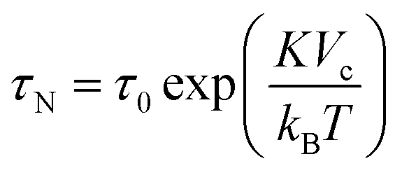
Two mechanisms are responsible for the thermal fluctuations measured in TNM. In liquid samples, the particles undergo Brownian motion. The MNPs, and thus their magnetic moments, rotate at time scales38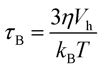 | (1) |
 | (2) |
 | (3) |
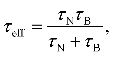
The magnetic TNM signal B measured over time is stochastic in nature with an autocorrelation function
GB(t) = 〈B(0)B(t)〉 = 〈B2〉![[thin space (1/6-em)]](https://www.rsc.org/images/entities/char_2009.gif) exp(−|t|/τeff). exp(−|t|/τeff). | (4) |
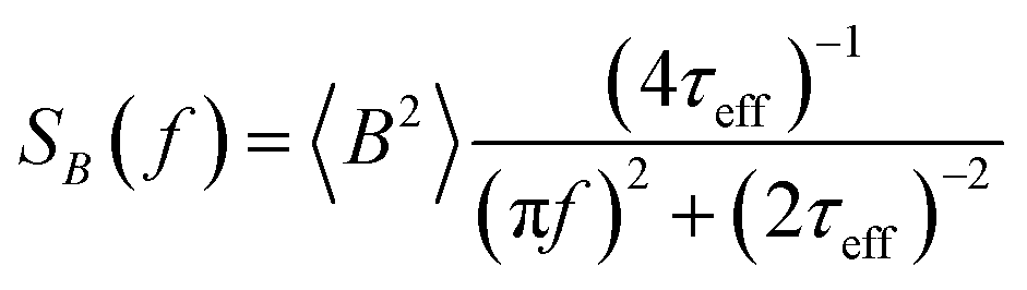
The power spectral density (PSD) is then obtained from the Wiener–Khintchine theorem as the Fourier transform of the autocorrelation function:40,41
 | (5) |
The amplitude 〈B2〉 of the fluctuations depends on the total magnetic moment of the MNPs, and the distance from the sample at which the magnetic field is measured. At typical distances of a few mm to a few cm, the TNM signal of the MNP ensemble ranges from pT to fT. Due to the stochastic nature of TNM, the amplitude of the fluctuations is given by the variance of the stochastic variable, which scales linearly with the amount of particles and quadratically with the volume of the fluctuators.31 Therefore, TNM is fundamentally more sensitive to clustering events than corresponding deterministic magnetic characterization methods.
The dynamics of the MNPs are quantified using the fluctuation time τeff, which also defines the width of the PSD. The cutoff frequency 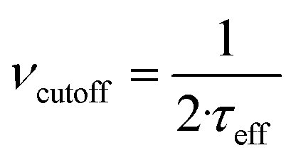 divides the PSD into two regimes: a low-frequency regime where f < νcutoff and a high-frequency regime where f > νcutoff. The PSD is flat in the low-frequency regime, as visualized by Fig. 1(1a). In the high-frequency regime, the PSD drops with 1/f2.
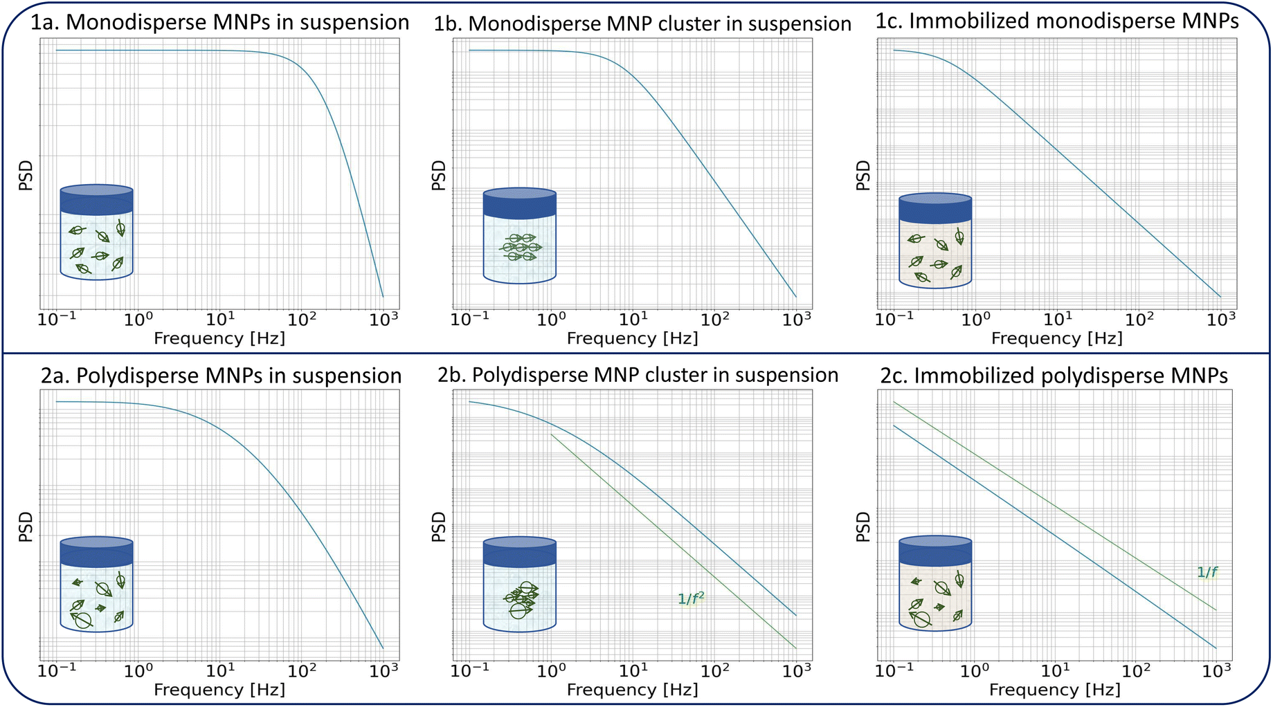 | ||
| Fig. 1 Theoretical noise spectra of different samples. The PSDs of the monodisperse particles (1a–c) are displayed for particles with a hydrodynamic diameter of dh = 130 nm and a core diameter of dc = 25 nm. The PSD is flat up to the characteristic cutoff frequency, after which it falls off with 1/f2. The diameters of the polydisperse particles (2a–c) follow a lognormal size distribution with parameters dh ∼ lnN(μ = 124 nm, σ = 0.35) and dc ∼ lnN(μ = 25 nm, σ = 0.45). In the case of polydisperse cluster formation (2b), the PSD still prominently has a 1/f2 shape. In the case of the immobilization of the polydisperse particles (2c), a typical 1/f shape is distinguished due to the extremely broad fluctuation time distribution. The diameter of the clusters was taken 3 times the diameter of the single particles. | ||
Direct parameters influencing the cutoff frequency of idealized non-interacting particles are those included in eqn (1) and (2). However, a change in the aggregation state or mobility of the particles, or an increase in the interparticle interaction, also affects their magnetization dynamics. Consequently, these processes must impact the noise spectrum as well. Fig. 1 shows the theoretical expression of the PSD for different MNP configurations to illustrate the changes. Particle clustering (Fig. 1(1b)) increases the hydrodynamic volume of the individual fluctuators with a decrease in the Brownian fluctuation time as a result. The cutoff frequency shifts towards smaller frequencies, and the 1/f2 behavior becomes more pronounced. Néel fluctuations are often orders of magnitude slower than Brownian rotations in most MNP systems (for the common case of iron oxide MNPs with large core diameters dc > 10 nm). This means that the cutoff frequency also shifts towards lower values upon elimination of Brownian rotations during immobilization (Fig. 1(1c)).
For a polydisperse sample, the volumes Vh and Vc are distributed along the distributions P(Vh) and P(Vc), and the corresponding fluctuation time τeff along P(τeff). The PSD for a non-interacting polydisperse MNP ensemble can then be written as a superposition of independent fluctuators (5)
 | (6) |
 | (7) |
This typically results in a stretching of the PSD in the cutoff region as visible in Fig. 1(2a). For a broad size- or fluctuation time distribution, the PSD finally can be approximated using a 1/f curve.29,42
Similar to clustering of monodisperse particles, the hydrodynamic size of a polydisperse cluster also increases, and its related cutoff frequency shifts towards lower frequency values. The 1/f2 falloff dominates in the considered bandwidth as shown in Fig. 1(2b). The effect of immobilization of a polydisperse sample is even more pronounced since the Néel fluctuation time depends exponentially on the core volume. The size distribution translates into a broad fluctuation time distribution, and the PSD gets the distinct 1/f shape which is displayed in Fig. 1(2c).
The superposition of individual fluctuators in eqn (6) and (7) does not hold if interparticle interactions are present in e.g. aggregates. The extraction of quantitative information about the involved interactions from their noise signals is beyond the scope of this work, but a qualitative effect of interparticle interactions on the measured PSD can be predicted. Interactions between moments that fluctuate by the Brownian mechanism will shift the cutoff frequency towards lower frequencies compared to the non-interacting case, as the coupled rotations result in a larger moment of inertia. Under the assumption that the particles aggregate in a configuration in which their anisotropy axes align in a way that results in a low-energy state, the interactions will increase the switching energy barriers for the Néel switching, resulting as well in lower switching rates. For both mechanisms, the cutoff frequencies in the spectrum shift to lower values than a mere superposition would suggest, thereby further increasing the sensitivity of the method to detect aggregations. The fitting of an effective size distribution to the PSD of an interacting system with eqn (7) would therefore overestimate the actual size distribution of the ensemble.
We would also like to point out that clustering, aggregation, and immobilization of MNPs are generally not uncorrelated and often occur at the same time. Together with broad size distributions, this makes the quantitative interpretation of the fluctuation dynamics of the magnetic moments less straightforward than for the model curves displayed in Fig. 1 where only one effect is considered.
2.2 Experimental setups
The developed tabletop setup (Fig. 3a) consists of two Gen-2 QuSpin zero-field magnetometers (QZFMs) (QuSpin Inc., CO, USA)58 that are operated in single-axis mode. One is placed in the center of the shield (QZFM1) and used to subsequently measure the background noise and the MNP noise. The other is used as a backup sensor for the differentiation between sensor-specific disturbances and environmental noise (QZFM2).
The QZFMs operate in the ultrasensitive spin exchange relaxation free (SERF) regime.59 SERF OPMs such as the QZFM have stringent demands on the magnetic shielding environment. The time-invariant remnant field inside the shield needs to be less than 50 nT. Additionally, the dynamic field changes down to the mHz-range, i.e. slow fluctuations, need to be less than 1.5 nT to achieve linear sensor gain.60 The numerical values of maximum remnant and maximum dynamic field are dependent on the specific design of the manufacturer's sensor electronics, but generally SERF sensors require two or more layers of magnetic shielding. In our setup, we tested that QZFM operation is possible by measuring field fluctuations over a 30-minute period and by observing the remnant field compensation values reported by the user interface of the QZFM sensor. Fluctuations in the 4-layer MS-2 laboratory shield were less than 50 pT and the remnant field was 5 nT for QZFM1 and 19 nT for QZFM2. The MS-2 has a dynamic shielding factor of 106 as specified by the manufacturer (Twinleaf LLC, NJ, USA61), which is sufficient in our urban environment. The difference in remnant field is not necessarily due to the shield but can be an intrinsic difference between individual sensors. Nevertheless, the sensors were operated as specified by the manufacturer.
The sample and the QZFMs are placed inside the MS-2 magnetic shield to minimize the effect of external fields on the MNPs dynamics and to ensure the proper working of the QZFMs as discussed above. The controlling QZFM electronics is placed outside the shield and driven via the QuSpin user interface program on a laptop, from which the data are also collected with a U6 Labjack (LabJack Corporation, CO, USA) in stream mode. The tabletop setup was operated in a conventional lab environment. The 50 Hz contamination from the power line and its related 150 Hz peak are visible in the measured background spectrum (Fig. 2a) on a noise floor of approx. 200–2000  (10–40
  ). Among other environmental disturbances, the 923 Hz signal from the QZFM modulation and its aliasing peak around 77 Hz are visible.† The manufacturer does not specify any product information of the QZFM above 100 Hz, because of the phase shift in the signal above this frequency. However, since our spectral measure is phase-insensitive, we are able to extend the bandwidth of the QZFM beyond its usual 100 Hz frequency range, as explained in Section 2.3. A spectral drop-off at frequencies above ∼500 Hz is a consequence of the lock-in detection technique used in the QZFM sensor design and electronics. It is the basis of the sensor's directional detection of the magnetic field. It relies on a field modulation at 923 Hz generated by the sensor head itself to alter the state of the Rb gas in the cell. Theoretically, however, signals above fmodulation/2 = 461 Hz cannot be resolved properly by a correlation calculation and the drop-off is certainly related to that, although the technical details are not disclosed by the manufacturer. Time signals of up to 20 minutes were recorded at a sample rate of 2 kHz, and the PSD was calculated and averaged as explained in the Methods section of ref. 31. The final displayed spectra are calculated by subtracting the background spectrum PSDBG from the MNP spectrum PSDMNP.
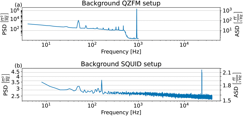 | ||
| Fig. 2 Background power spectral density in the tabletop QZFM setup (a). The 50 Hz contamination from the power line and its related 150 Hz peak are visible amongst other environmental disturbances. The 923 Hz signal from the QZFM modulation and its aliasing peak around 77 Hz. (b) Background of the in-house developed SQUID setup. The 50 and 150 Hz peaks from power line residuals are visible, as well as two peaks around 24 kHz. | ||
To achieve an optimal Rb density for increased sensitivity, the QZFM vapor cell is heated to a temperature of about 160 °C.58,62 This has an immediate effect on the temperature of the sample, and overheating of the MNPs is prevented by placing a 2 mm thick insulation material between the housing of the QZFM and the sample. A sample temperature of 43.2 ± 0.5 °C was measured after a stabilization time of 20 minutes after placement in the setup. With the insulation material included, the minimal distance between the centre of the vapor cell and the sample is estimated to be 8.5 mm. With a sample height of approximately 10 mm, the average distance between the centre of the vapor cell and the MNPs is 13.5 mm.
 (1.5–1.8
  ). 50 and 150 Hz peaks from power line residuals are visible, as well as two peaks around 24 kHz (Fig. 2b). As is clear from eqn (1) and (2), the dynamics of the particles is strongly dependent on the temperature. To compare both measurement systems under the same conditions, the sample has been kept at a constant temperature of 43.0 ± 0.5 °C in the SQUID setup to match the sample temperature in the QZFM setup. This was achieved by the use of a stable airflow through the sample bore. Magnetic signals of 13 minutes were acquired at a sample rate of 100 kHz and the PSDs were subsequently calculated and averaged.
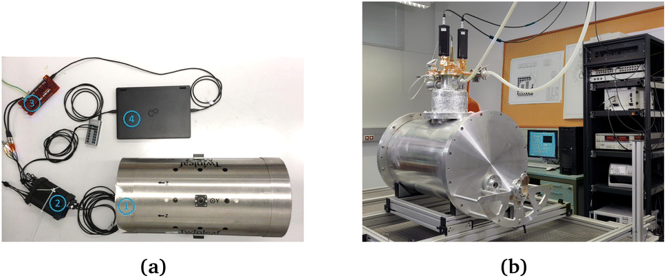 | ||
| Fig. 3 (a) Tabletop TNM setup based on OPMs. The sample is placed inside the Twinleaf MS-2 shield (1) together with the two QZFMs. QZFM electronics (2) control the sensors and a laptop (4) serves for driving the DAQ Labjack U6 (3) in stream mode, running the QZFM electronics and collecting the data. The sample is at an average distance of 13.5 mm from the gas cell with the polarized Rb atoms. (b) In-house developed SQUID setup for reference measurements. A superconducting Nb magnetic shield and 6 SQUID sensors are kept at LHe temperature; the sample is placed in a bore through the setup and kept at an average temperature of 43.0 ± 0.5 °C to match the sample temperature in the tabletop setup. An average distance of 23.5 mm is measured between the pickup coils of the SQUID sensors and the sample. Only one sensor is used for the TNM measurement. | ||
2.3 Frequency response of the sensors
The operation of the OPMs is generally limited to approximately 100 Hz ‡ due to phase instability above this frequency. However, the spectral measure used in TNM is phase insensitive. By accounting for the frequency response profile of the magnetometers, a bandwidth of up to 514 Hz can be employed. In this section, we explain how we measured and used the frequency response profile of the QZFMs for TNM applications.First, a frequency response profile of the QZFMs has been measured to ensure a quantitatively correct measurement of the power spectra of the MNPs. To this end, the sensors were placed inside a magnetically shielded room at the Physikalisch-Technische Bundesanstalt (named as the “Zuse-MSR” in ref. 64) and a homogeneous AC field with an amplitude of 772 pT was applied by the use of a square Helmholtz coil. Its frequency was swept in the range of [2–600] Hz. The amplitude of the QZFM output signal was monitored and analyzed in the time domain, after which the response values were averaged and normalized. From this data set, a frequency response profile was calculated for both QZFMs as shown in Fig. 4. The uncertainty in the response values was calculated from the standard deviation of the different peaks of the excitation and the response at one frequency. Note that the frequency response varies strongly and differently for both QZFMs and that there is a 10% gain variation at frequencies up to 100 Hz. For comparison, a similar procedure was performed with the SQUID sensor with a field of 60 pT by inserting a small coil into the warm bore. There was no frequency dependence of the amplitude detected as can be seen in Fig. 4. The power spectral density SB(f) of a MNP ensemble can then be calculated by correcting for the frequency response of the QZFMs
 | (8) |
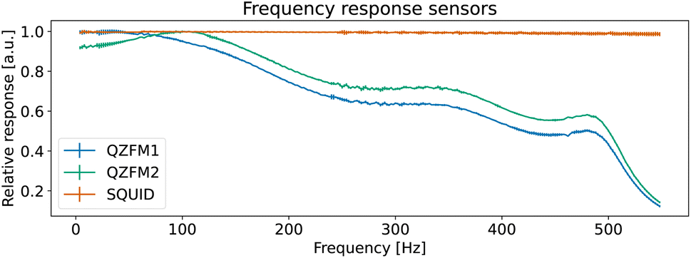 | ||
| Fig. 4 Measured frequency responses H(f) of the different sensors. The data were acquired by application of an AC magnetic field with sweeping frequency. | ||
3 Results and discussion
3.1 Comparison of power spectra
Fig. 5(a) shows the power spectral densities of both MNP systems measured in the SQUID setup. For the displayed MNP noise spectra, the background PSDBG was subtracted. The PSD of the FCT system is relatively flat up to a cutoff frequency of about 90 Hz, after which the PSD starts to decrease continuously due to the size distribution of the particles. The Perimag® system shows higher power at lower frequencies, with the cutoff frequency located at values lower than the displayed frequency resolution. This is a result of the slower magnetization dynamics due to the large hydrodynamic size of the Perimag® particles with a broad size distribution, as explained by eqn (7).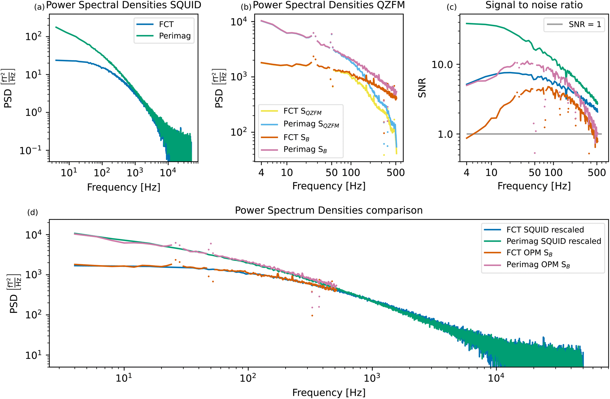 | ||
| Fig. 5 Measured SQUID spectra of the two MNP systems (a) and measured and compensated QZFM profiles of the two MNP systems (b). For clarity, the points in the QZFM spectra at the interfering background frequencies (30, 50, 330, and 375 Hz) have been plotted separately. These correspond to the peaks in the background spectrum of the tabletop setup in Fig. 2. The signal-to-noise ratio (SNR) of (a) and (b) is plotted in (c). Qualitative comparison of the MNP spectra measured in both setups (d). The SQUID spectra of (a) have been rescaled to match the power of the OPM spectra SB in (b) at 80 Hz. Apart from the interfering background peaks in the OPM spectra, a very good agreement between the measurements obtained in both setups is visible. | ||
It is not possible to compare the PSDs purely qualitatively by normalizing them to the iron content of the sample, as it is common for other characterization techniques. For deterministic processes, the signal depends linearly on both the number of magnetic moments and their amplitude, and thus also linearly on the iron concentration. However, TNM is a stochastic method, and the signal depends only on the square root of the number of magnetic moments.31 Therefore, if only the iron concentration of the sample is known, the number of magnetic moments and the amplitude of the moments cannot be decoupled, and a meaningful normalization is impossible. The PSDs of the samples are thus shown in their absolute values, although the Perimag® sample was more concentrated than the FCT sample.
The same MNP systems are measured in the tabletop setup. Fig. 2(a) shows a clear drop in the signal around 500 Hz. A value of −3 dB is reached at 514 Hz, which is why we choose to plot the MNP spectra up to this frequency. The spectra before (SQZFM(f)) and after the frequency response correction detailed in Section 2.3 (SB(f)) are displayed in Fig. 5(b).
Due to the reduced sample-sensor distance, the MNP signal is higher in the tabletop setup than in the SQUID system. However, the tabletop setup is less sensitive than the SQUID setup. This is clear from Fig. 5(c), which shows the signal-to-noise ratio (SNR) as a function of frequency for both setups and both MNP systems:
 | (9) |
The excellent performance of the SQUID setup becomes visible in the SNR plots. Both MNP systems have a SNR up to one order of magnitude higher in the SQUID setup compared to the tabletop OPM setup, even if the signal is two orders of magnitude lower. The tabletop setup has a steeper SNR loss than the SQUID setup above 100 Hz. Not only the signal, but also the noise is amplified as a result of the frequency response compensation. The SNR loss towards lower frequencies is also limited in the SQUID setup due to the advanced shielding by the superconducting shield.
In order to assess the suitability of a setup to investigate a particular MNP system, we use the criterion that SNR > 1. Perimag® will be used for the proof-of-concept experiments, since the SNR of FCT is relatively low in the lower frequency range in the tabletop setup. Moreover, the SNR of Perimag® above 400 Hz also crosses the SNR = 1 limit. For lower concentrated samples, such as those used in the proof-of-concept experiments, this crossing will occur even at lower frequencies.
The measurements are directly compared in Fig. 5(d) by rescaling the SQUID spectra to match the OPM spectra at 80 Hz. As the curves of the two particle systems measured in two setups overlap nicely, we conclude that the compensation for the frequency response profile of the QZFM is a valid approach. Despite their loss in sensitivity above 100 Hz, the QZFMs recover a quantitatively correct spectrum. For MNP samples with high power in the lower frequency range, such as the Perimag® and FCT samples used as example MNP systems here, both measurement systems are thus equally suitable. For smaller MNP systems with dynamics in the higher frequency range, the tabletop setup might not be sufficient, both in bandwidth and sensitivity. However, these particle systems could still be studied in the tabletop setup by increasing the viscosity of the suspension, as proposed in ref. 30.
3.2 Monitoring of clustering processes
Since the TNM signal scales quadratically with the volume of the noise sources,31 this technique is particularly suited to monitor the clustering processes of magnetic nanoparticles. The absence of any driving field during the measurement also excludes any undesired effects induced by an external excitation. Moreover, the good performance of the QZFM at lower frequencies favours the monitoring of processes which tend to slow down the magnetization dynamics of the sample. An OPM-based TNM setup thus offers a broadly applicable tool to monitor the clustering of MNPs. As a proof of concept, we report on the monitoring of three such processes, measured with TNM in the described tabletop setup:1. Enforced aggregation of Perimag® particles by addition of ethanol.
2. Formation of photopolymer structures in a Perimag® sample by exposure to UV light.
3. Cellular uptake of Perimag® particles by THP-1 cells.
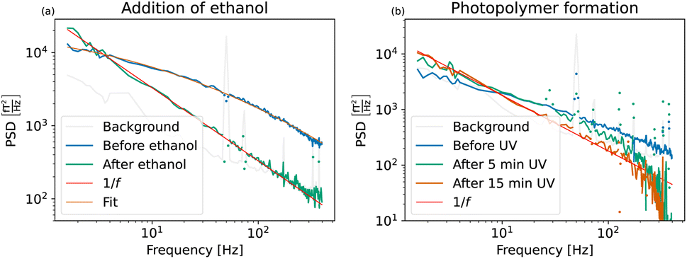 | ||
| Fig. 6 (a) Power spectral densities of Perimag® particles before and after addition of ethanol. A lognormal size distribution with an average diameter of 101 ± 26.0 nm was fitted to the MNP sample before aggregation. After the addition of ethanol, the magnetic cores aggregate and sediment due to gravity. Due to the extremely broad distribution of the Néel fluctuation times, the PSD has a distinct 1/f shape as shown in Fig. 1(2c). (b) Power spectral densities of Perimag® particles before and after polymer formation. A gradual immobilization of the particles is induced during UV curing and full immobilization is reached after 15 minutes of exposure time. | ||
A lognormal size distribution logN(μ = 72.6 ± 5 nm, σ = 0.82 ± 0.3) with an average hydrodynamic diameter of 101 ± 26.0 nm was fitted to the curve before the addition of ethanol. Given the limited bandwidth of 400 Hz, these parameters match the average diameter of 130 nm of the manufacturer reasonably well.
After the addition of ethanol, the aggregates sediment and only undergo Néel fluctuations. Their noise curve is dominated by 1/f noise. The slow magnetization dynamics of the aggregated MNPs and the broad size distribution of their fluctuation times are distinctive signatures of this process which is depicted schematically in Fig. 1(2c).
First, the Perimag®-photopolymer mixture was prepared by adding 100 μl Perimag® sample with an iron concentration of 644.4 mmol l−1 to a 100 μl photopolymer base material § in a 2 ml Eppendorf tube. A homogeneous spatial distribution of the particles in the base material was ensured by sonication with an ultrasound sonifier (UP200Ht, Hielscher Electronics, Germany). 120 μl of the mixture was used as a sample and the first spectrum was measured before UV exposure. The sample was then exposed to UV light in a UVACUBE 2000 for 5 and 10 minutes subsequently.
Fig. 6(b) shows the measured spectra of the particles in the base material before exposure, and after 5 and 15 minutes of total exposure time. Since only 60 μl magnetic material has been used in this experiment, the TNM signal amplitude is lower than in the spectra shown previously. Therefore, we argue that the falloff above 200 Hz of the two exposure spectra is an artificial effect due to insufficient SNR and not the physical shape of the spectra, which we expect to decrease linearly on the log–log scale.
Before UV exposure, the particles rotate freely in the highly viscous base material. Compared to the water-suspended particles in Fig. 6(a), their Brownian rotations are slower. The related cutoff frequency is shifted to lower frequencies outside the window, and only the straight tail of the PSD is visible. Brownian movement of the particles is further excluded due to crosslink formation as the MNPs get enclosed in small polymer cavities during UV curing. The effective viscosity increases towards an eventual full immobilization. The Brownian fluctuations gradually slow down, the related Brownian cutoff frequency moves closer towards DC values and Néel fluctuations become dominant. After 15 minutes of exposure time, the PSD reaches the limiting 1/f shape in Fig. 6(b). All particles are immobilized, as the PSD is directly comparable with the PSD of the aggregates in Fig. 6(a).
During UV curing, the volume and geometry of the sample are conserved and the spectra can be compared quantitatively. This allows us to define an effective immobilization degree based on the PSD value at a stable low frequency after each exposure step. A comparison of the PSD values at 1.6 Hz of the sample before exposure and after five minutes of exposure time to the PSD value at 1.6 Hz of the fully immobilized state gives an immobilization of 50% and 72%, respectively. This experiment therefore shows the potential of TNM to be used for continuous monitoring during MNP clustering and immobilization processes.
200 μL COOH coated Perimag® particles with a concentration of c(Fe) = 244.7 mmol l−1 were incubated with 2 × 10⁷ THP-1 cells in a 800 μl RPMI + 1% FCS medium for 24 hours. Fig. 7 shows the cells before and after the incubation (undiluted sample), where iron is visualized by Prussian blue staining. From these pictures, it is clear that the magnetic nanoparticles are taken up by the cells to a great extent. Moreover, MNPs in the surrounding solution also form aggregates.
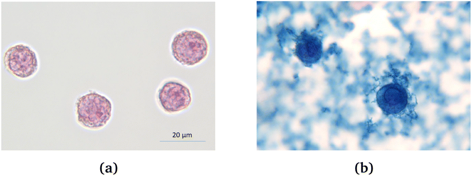 | ||
| Fig. 7 THP-1 cells without (a) and with (b) addition of Perimag® particles after 24 hours of incubation time. Iron in the sample is visualized by Prussian Blue staining. The particles are to a great extent taken up by the cells. Redundant particles outside the cells still form aggregates, being attached to the outer wall of the cells. | ||
Three different samples have been measured in the tabletop TNM setup and are displayed in Fig. 8 with their respective colours:
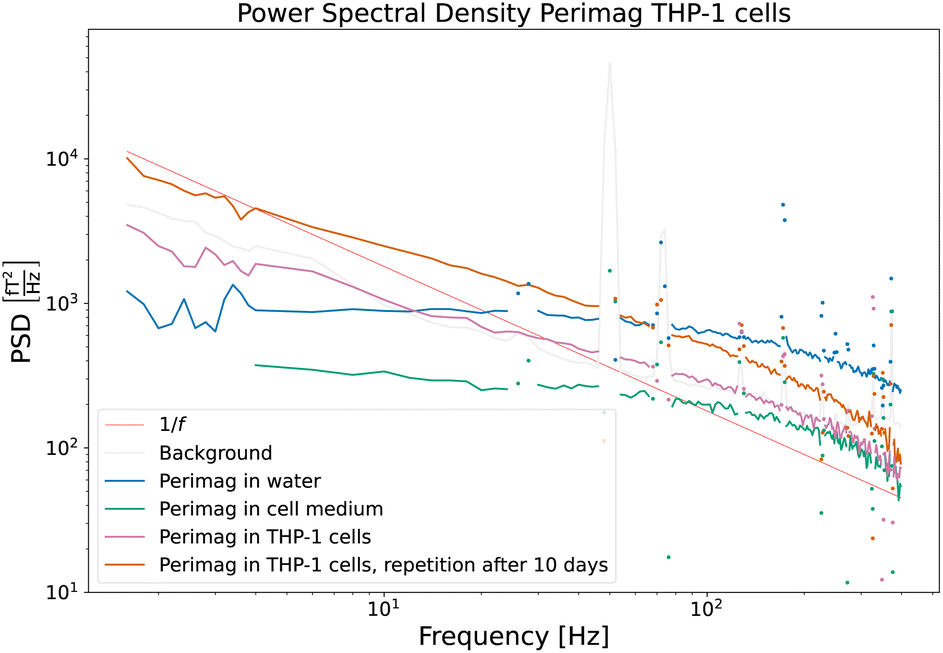 | ||
| Fig. 8 Power spectral densities of COOH coated Perimag® particles before and after cellular uptake by THP-1 cells. The influence of the cell medium on the dynamics of the particles is very limited. Due to cluster formation and partial immobilization of the particles after cellular uptake, the power in the lower frequency range increases. Full immobilization is however excluded, since the distinctive 1/f behaviour of Fig. 6 is not reached. | ||
(A) Perimag® particles in water suspension (blue).
(B) Perimag® particles in the cell medium (green).
(C) Perimag® particles after 24 h of incubation time with THP-1 cells (pink).
The PSD of the particles in the water suspension and the cell medium shows only quantitative differences, which are due to the difference in concentration of the samples. The influence of the cell medium on the dynamics of the particles is – at least in the measured frequency range – very limited. After cellular uptake of the particles by the cells, a higher relative noise power in the lower frequency regime is measured, and the faster fluctuations are less present in the noise spectrum. The broad distribution of cutoff frequencies clearly shifts towards lower values, which can be attributed to the formation of clusters and partial immobilization. Full immobilization can however be excluded, since the PSD does not fall off with 1/f as in Fig. 6(a) and (b). A repetition measurement of Sample C was carried out after 10 days (orange curve). Apart from an increased SNR – which is related to the further cell sedimentation and a decreased average sample sensor distance – no qualitative differences were detectable. The magnetization dynamics of the particles in the well-aged cell sample shows no notable differences from that of the sample directly after the 24 h incubation.
Two noise curves can be compared quantitatively, namely those of the particles suspended in the cell medium and those of the particles directly after the incubation time, because the MNP concentration and sample volume were similar. A continuous probing of the noise power at e.g. 10 Hz could quantify the cellular uptake during the incubation process.
4 Conclusion and outlook
Thermally induced magnetic noise of two commercially available MNP systems was measured in the presented OPM-based tabletop setup. A good agreement was found with the noise spectra measured with SQUIDs. These are the first thermal noise spectra of MNP ensembles measured with OPMs. Three proof-of-principle experiments conducted in the tabletop setup show the effect of particle clustering, immobilization and cellular uptake on the thermal noise of the MNP ensemble.Presently, for a detailed MNP characterization by TNM, the SQUID setup remains preferred because of its wide bandwidth, which allows for the mapping of a broad range of MNP systems, and higher sensitivity, which facilitates the investigation of lower concentrated samples. An OPM sensor specifically designed for TNM could be more suited than the broadly applicable commercial magnetometers used in this study. Although a simultaneous optimization of bandwidth and sensitivity is not possible due to their inverse relation,35 an optimum between them can be found for different MNP systems with different characteristic noise spectra. Moreover, due to the isotropy of the MNP noise, a likewise measurement setup does not benefit from a vector magnetometer. Therefore, the vectorial sensitivity could be given up in favor of the scalar bandwidth and sensitivity. Further work will be dedicated to this.
However, OPM sensors are well suited to monitor the clustering and aggregation of MNPs by TNM. TNM is particularly sensitive to particle clustering because the amplitude of the signal increases with the square of the volume of the individual fluctuators, which means that an aggregate of two particles results in a signal that is twice as large as the sum of their individual signals. Moreover, no external excitation is required during the TNM measurement procedure, which could influence the clustering process itself or falsely influence the outcome of the measurement. Secondly, the excellent low-frequency performance of OPMs favors particle systems with slow dynamics or processes which tend to slow down the dynamics of the magnetic entities in the sample. Typical examples of these processes are found when the MNPs come in contact with biological systems, e.g. for biomedical purposes. Finally, the setup can be operated anywhere with a conventional power outlet due to the OPM flexibility and can thus also be used to track processes that require environmental and experimental freedom.
The immobilization of the particles induces a distinct 1/f dependency in the power spectral density, which results from the broad distribution of the Néel fluctuation times, as is visible from the gradual formation of UV polymers in a MNP sample. In contrast, the clustering of the particles when taken up by THP-1 cells slows down the Brownian fluctuations, due to the increased volume of the fluctuators, with a shift of the corresponding cutoff frequency towards lower frequencies as a result.
The OPM-based tabletop setup offers a flexible measurement unit to track changes in the thermal noise spectra of magnetic nano- and microsystems. Due to the non-invasive noise-based method and the simplicity of the setup, the unit is broadly adaptable and suited for the tracking of processes beyond biomedical applications, e.g. the long-term stability of magnetic samples.
Author contributions
K. Everaert: conceptualization, formal analysis, investigation, methodology, validation, visualization, writing – original draft; T. Sander: conceptualization, investigation, resources, validation; R. Körber: investigation, resources, validation; N. Löwa: conceptualization, resources; B. Van Waeyenberge: supervision, writing – review & editing; J. Leliaert: conceptualization, funding acquisition, methodology, supervision, writing – review & editing; F. Wiekhorst: conceptualization, funding acquisition, methodology, resources, supervision, writing – review & editing.Conflicts of interest
There are no conflicts to declare.Acknowledgements
This work was supported by the German Research Foundation (DFG) through the Project “MagNoise: Establishing Thermal Noise Magnetometry for Magnetic Nanoparticle Characterization” under Grant FKZ WI4230/3-1. J. L. was supported by the Fonds Wetenschappelijk Onderzoek (FWO-Vlaanderen) with senior postdoctoral research fellowship No. 12W7622N. We thank Prof. Dr Antje Ludwig and Lena Kampen from Charité University Hospital Berlin for their help with the cell experiments and Prof. Dr Samo Beguš from the University of Ljubljana for fruitful discussions concerning the shielding of the tabletop setup.Notes and references
- A. Jordan, R. Scholz, P. Wust, H. Fähling and R. Felix, J. Magn. Magn. Mater., 1999, 201, 413–419 CrossRef CAS.
- Q. A. Pankhurst, J. Connolly, S. K. Jones and J. Dobson, J. Phys. D: Appl. Phys., 2003, 36, 167–181 CrossRef.
- A. Ito, M. Shinkai, H. Honda and T. Kobayashi, J. Biosci. Bioeng., 2005, 100, 1–11 CrossRef CAS PubMed.
- Q. A. Pankhurst, T. K. Thanh, S. K. Jones and J. Dobson, J. Phys. D: Appl. Phys., 2009, 42, 224001 CrossRef.
- T. K. Thanh, Clinical Applications of Magnetic Nanoparticles, CRC Press, 2018 Search PubMed.
- S. Tong, H. Zhu and G. Bao, Mater. Today, 2019, 31, 86 CrossRef CAS PubMed.
- S. Caspani, R. Magalhães, J. P. Araújo and C. T. Sousa, Materials, 2019, 13, 2586 CrossRef PubMed.
- A. Coene and J. Leliaert, J. Appl. Phys., 2022, 131, 160902 CrossRef CAS.
- M. L. Etheridge, K. R. Hurley, J. Zhang, S. Jeon, H. L. Ring, C. Hogan, C. L. Haynes, M. Garwood and J. C. Bischof, Technology, 2014, 2, 214–228 CrossRef PubMed.
- S. Majetich and S. Sachan, J. Phys. D: Appl. Phys., 2006, 39, 407–422 CrossRef.
- D. Eberbeck, F. Wiekhorst, U. Steinhoff and L. Trahms, J. Phys.: Condens. Matter, 2006, 18, 2829–2846 CrossRef.
- S. Mørup, C. Hansen and C. Frandsen, Beilstein J. Nanotechnol., 2010, 1, 182–190 CrossRef PubMed.
- U. M. Engelmann, E. M. Buhl, S. Draack, T. Viereck, F. Ludwig, T. Schmitz-Rode and I. Slabu, IEEE Magn. Lett., 2018, 9, 1507305 CAS.
- L. Gutiérrez, L. de la Cueva, M. Moros, E. Mazarío, S. de Bernardo, J. M. de la Fuente, M. Puerto Morales and G. Salas, Nanotechnology, 2019, 30, 112001 CrossRef PubMed.
- N. Löwa, F. Wiekhorst, I. Gemeinhardt, M. Ebert, J. Schnorr, S. Wagner, M. Taupitz and L. Trahms, IEEE Trans. Magn., 2013, 49, 275–278 Search PubMed.
- H. Paysen, N. Löwa, A. Stach, J. Wells, O. Kosch, S. Twamley, M. R. Makowski, T. Schaeffter, A. Ludwig and F. Wiekhorst, Sci. Rep., 2020, 10, 1922 CrossRef CAS PubMed.
- D. Cabrera, J. Camarero, D. Aortega and F. J. Teran, J. Nanopart. Res., 2015, 17, 121 CrossRef.
- D. Cabrera, A. Lak, M. E. Materia, D. Ortega, F. Ludwig, P. Guardia, A. Sathya, T. Pellegrino and F. J. Teran, Nanoscale, 2017, 9, 5094 RSC.
- P. Bender, J. Fock, M. F. Hansen, L. K. Bogart, P. Southern, F. Ludwig, F. Wiekhorst, W. Szczerba, L. J. Zeng, D. Heinke, N. Gehrke, M. T. Díaz, D. González-Alonso, J. I. Espeso, J. R. Fernández and C. Johansson, Nanotechnology, 2018, 29, 425705 CrossRef CAS PubMed.
- D. Cabrera, A. Coene, J. Leliaert, E. J. Artés-Ibáñez, L. Dupré, N. D. Telling and F. J. Teran, ACS Nano, 2018, 12(3), 2741–2752 CrossRef CAS PubMed.
- U. M. Engelmann, J. Seifert, B. Mues, S. Roitsch, C. Ménager, A. M. Schmidt and I. Slabu, J. Magn. Magn. Mater., 2019, 471, 486–494 CrossRef CAS.
- R. Mejías, P. Hernandez Flores, M. Talelli, J. L. Tajada-Herraiz, M. E. F. Brollo, Y. Portilla, M. P. Morales and D. F. Barber, ACS Appl. Mater. Interfaces, 2019, 11, 340–355 CrossRef PubMed.
- J. Ortega-Julia, D. Ortega and J. Leliaert, arXiv, 2022, preprint, arXiv:2207.14551, DOI:10.48550/arXiv.2207.14551.
- F. Wiekhorst, U. Steinhoff, D. Eberbeck and L. Trahms, Pharm. Res., 2012, 29, 1189–1202 CrossRef CAS PubMed.
- F. Ludwig, D. Eberbeck, N. Löwa, U. Steinhoff, T. Wawrzik, M. Schilling and L., Trahms, Biomed. Tech. (Berl), 2013, 58, 535–545 Search PubMed.
- F. Ludwig, C. Balceris, C. Jonasson and C. Johansson, IEEE Trans. Magn., 2017, 53(11), 6100904 Search PubMed.
- H. Mamiya, H. Fukumoto, J. L. Cuya Huaman, K. Suzuki, H. Miyamura and J. Balachandran, ACS Nano, 2020, 14, 8421–8432 CrossRef CAS PubMed.
- T. Q. Bui, A. J. Biacchi, C. L. Dennis, W. L. Tew, A. R. Hight Walker and S.I. Woods, Appl. Phys. Lett, 2022, 120, 12407 CrossRef CAS PubMed.
- J. Leliaert, A. Coene, M. Liebl, D. Eberbeck, U. Steinhoff, F. Wiekhorst, B. Fischer, L. Dupré and B. Van Waeyenberge, Appl. Phys. Lett., 2015, 107, 222401 CrossRef.
- J. Leliaert, D. Eberbeck, M. Liebl, A. Coene, U. Steinhoff, F. Wiekhorst, B. Van Waeyenberge and L. Dupré, J. Phys. D: Appl. Phys., 2017, 50, 085004 CrossRef.
- K. Everaert, M. Liebl, D. Gutkelch, J. Wells, B. Van Waeyenberge, F. Wiekhorst and J. Leliaert, IEEE Access, 2021, 9, 111505–111517 Search PubMed.
- D. Cohen, Science, 1972, 175, 664–666 CrossRef CAS PubMed.
- M. Burghoff, H. H. Albrecht, S. Hartwig, I. Hilschenz, R. Körber, T. S. Thömmes, H. J. Scheer, J. Voigt and L. Trahms, Metrol. Meas. Syst., 2009, XVI(3), 371–375 Search PubMed.
- R. Körber, J. H. Storm, H. Seton, J. P. Makela, R. Paetau, L. Parkkonen, C. Pfeiffer, B. Riaz, J. F. Schneiderman, H. Dong, S. M. Hwang, L. You, B. Inglis, J. Clarke, M. A. Espy, R. J. Ilmoniemi, P. E. Magnelind, A. Matlashov, J. O. Nieminen, P. L. Volegov, K. C. Zevenhoven, N. Höfner, M. Burghoff, K. Enpuku, S. Y. Yang, J. Chieh, J. Knuutila, P. Laine and J. Nenonen, Supercond. Sci. Technol., 2016, 29, 113001 CrossRef.
- D. Budker and M. Romalis, Nat. Phys., 2007, 3, 227–234 Search PubMed.
- T. Tierney, N. Holmes, S. Mellor, J. D. López, G. Roberts, R. M. Hill, E. Boto, J. Leggett, V. Shah, M. J. Brookes, R. Bowtell and G. R. Barnes, NeuroImage, 2019, 199, 598–608 CrossRef PubMed.
- E. Boto, N. Holmes, J. Leggett, G. Roberts, V. Shah, S. S. Meyer, L. D. Muñoz, K. J. Mullinger, T. M Tierney, S. Bestmann, G. R. Barnes, R. Bowtell and M. J. Brookes, Nature, 2018, 555, 657–661 CrossRef CAS PubMed.
- P. Debye, Polar Molecules, Chemical Catalog Company, New York, 1929 Search PubMed.
- W. F. Brown, Phys. Rev., 1963, 130, 1677–1686 CrossRef.
- N. Wiener, Acta Math., 1930, 55, 117–258 Search PubMed.
- A. Khintchine, Math. Ann., 1934, 109, 604–615 CrossRef.
- M. B. Weissman, Rev. Mod. Phys., 1988, 60, 537–571 CrossRef CAS.
- T. Yoshida, K. Enpuku, F. Ludwig, J. Dieckhoff, T. Wawrzik, A. Lak and M. Schilling, Characterization of Resovist® Nanoparticles for Magnetic Particle Imaging, 2012 Search PubMed.
- D. Eberbeck, C. L. Dennis, N. F. Huls, K. L. Krycka, C. Grüttner and F. Westphal, IEEE Trans. Magn., 2013, 49, 269–274 Search PubMed.
- T. Sander, A. Jodko-Władzińska, S. Hartwig, R. Brühl and T. Middelmann, Adv. Opt. Technol., 2020, 9, 247–251 CrossRef.
- C. Deans, Y. Cohen and H. Yao, Appl. Phys. Lett., 2021, 119, 014001 CrossRef CAS.
- P. J. Broser, T. Middelmann, D. Sometti and C. Braun, J. Electromyogr. Kinesiology, 2021, 56, 102490 CrossRef PubMed.
- M. G. Bason, T. Coussens, M. Withers, C. Abel, G. Kendall and P. Krüger, J. Power Sources, 2022, 533, 231312 CrossRef CAS.
- S. Knappe, T. Sander, O. Kosch, F. Wiekhorst, J. Kitching and L. Trahms, Appl. Phys. Lett., 2010, 97, 133703 CrossRef.
- R. M. Hill, E. Boto, M. Rea, N. Holmes, J. Leggett, L. A. Coles, M. Papastavrou, S. K. Everton, B. A. Hunt, D. Sims, J. Osborne, V. Shah, R. Bowtell and M. J. Brookes, NeuroImage, 2020, 219, 116995 CrossRef PubMed.
- U. Marhl, A. Jodko-Władzińska, R. Brühl, T. Sander and V. Jazbinš Ek, Plos One, 2022, 17, e0262669 CrossRef CAS PubMed.
- C. Johnson, N. L. Adolphi, K. L. Butler, D. M. Lovato, R. Larson, P. D. Schwindt and E. R. Flynn, J. Magn. Magn. Mater., 2012, 324, 2613–2619 CrossRef CAS PubMed.
- V. Dolgovskiy, V. Lebedev, S. Colombo, A. Weis, B. Michen, L. Ackermann-Hirschi and A. Petri-Fink, J. Magn. Magn. Mater., 2015, 379, 137–150 CrossRef CAS.
- L. Bougas, L. D. Langenegger, C. A. Mora, W. J. Stark, A. Wickenbrock, J. W. Blanchard and D. Budker, Sci. Rep., 2018, 8, 3491 CrossRef PubMed.
- O. Baffa, R. H. Matsuda, S. Arsalani, A. Prospero, J. R. Miranda and R. T. Wakai, J. Magn. Magn. Mater., 2019, 475, 533–538 CrossRef CAS.
- A. Jaufenthaler, P. Schier, T. Middelmann, M. Liebl, F. Wiekhorst and D. Baumgarten, Sensors, 2020, 20, 753 CrossRef CAS PubMed.
- A. Jaufenthaler, V. Schultze, T. Scholtes, C. B. Schmidt, M. Handler, R. Stolz and D. Baumgarten, EPJ Quantum Technol., 2020, 7, 12 CrossRef.
- V. K. Shah and R. T. Wakai, Phys. Med. Biol., 2013, 58, 8153–8161 CrossRef PubMed.
- I. K. Kominis, T. W. Kornck, J. C. Allred and M. V. Romalis, Nature, 2003, 422, 596–599 CrossRef CAS PubMed.
- J. Osborne, J. Orton, O. Alem and V. Shah, Fully integrated standalone zero field optically pumped magnetometer for biomagnetism, Steep Dispersion Engineering and Opto-Atomic Precision Metrology XI, SPIE, 2018, vol. 10548 Search PubMed.
- MS-2 Magnetic shield, https://twinleaf.com/shield/MS-2/.
- A. Borna, T. R. Carter and J. D. Goldberg, Meas. Sci. Technol., 2017, 28, 035104 CrossRef.
- R. Ackermann, F. Wiekhorst, A. Beck, D. Gutkelch, F. Ruede, A. Schnabel, U. Steinhoff, D. Drung, J. Beyer, C. Aßmann, L. Trahms, H. Koch, T. Schurig, R. Fischer, M. Bader, H. Ogata and H. Kado, IEEE Trans. Appl. Supercond., 2007, 17, 827–830 CAS.
- J. Voigt, S. Knappe-Grüneberg, D. Gutkelch, J. Haueisen, S. Neuber, A. Schnabel and M. Burghoff, Rev. Sci. Instrum., 2015, 86, 55109 CrossRef CAS PubMed.
- N. Löwa, J. M. Fabert, D. Gutkelch, H. Paysen, O. Kosch and F. Wiekhorst, J. Magn. Magn. Mater., 2019, 469, 456–460 CrossRef.
- M. Ardila, D. Gutkelch, O. Kosch, F. Wiekhorst and N. Löwa, Polymers, 2022, 14, 3925 CrossRef PubMed.
- R. Di Corato, A. Espinosa, L. Lartigue, M. Tharaud, S. Chat, T. Pellegrino, C. Ménager, F. Gazeau and C. Wilhelm, Biomaterials, 2014, 35, 6400–6411 CrossRef CAS PubMed.
- W. C. Poller, N. Löwa, F. Wiekhorst, M. Taupitz, S. Wagner, K. Möller, G. Baumann, V. Stangl, L. Trahms and A. Ludwig, J. Biomed. Nanotechnol., 2016, 12, 337–346 CrossRef PubMed.
- E. Teeman, C. Shasha, J. E. Evans and K. M. Krishnan, Nanoscale, 2019, 11, 7771–7780 RSC.
- L. Moor, S. Scheibler, L. Gerken, K. Scheffler, F. Thieben, T. Knopp, I. Herrmann and F. Starsich, Nanoscale, 2022, 14, 7163–7173 RSC.
- A. Remmo, N. Löwa, O. Kosch, D. Eberbeck, A. Ludwig, L. Kampen, C. Grüttner and F. Wiekhorst, Cells, 2022, 11, 2892 CrossRef CAS PubMed.
Footnotes |
| † These disturbances can be minimized further by placing the shield in an aluminum cage, and grounding both the shield and the cage to the USB ground of the laptop. |
| ‡ This is 135 Hz for the QZFMs specifically, from personal communication with QuSpin Inc., CO, USA. |
| § Perfactory acrylic R5 red from EnvisionTEC Inc., composed of acrylic acid esters and a photoinitiator (0.1–5%). The Perfactory Acryl R5 resin has a density of 1.12–1.13 g cm−3. |
| This journal is © The Royal Society of Chemistry 2023 |