 Open Access Article
Plot2Spectra: an automatic spectra extraction tool
Weixin
Jiang
*ab,
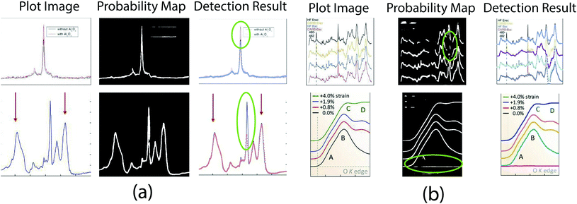
Kai
Li
c,
Trevor
Spreadbury
b,
Eric
Schwenker
b,
Oliver
Cossairt
a and
Maria K. Y.
Chan
 *b
*b
aDepartment of Computer Science, Northwestern University, Illinois, USA. E-mail: weixinjiang2022@u.northwestern.edu
bCenter for Nanoscale Materials, Argonne National Laboratory, Illinois, USA. E-mail: mchan@anl.gov
cReality Labs, Meta, California, USA
First published on 23rd August 2022
Abstract
Different types of spectroscopies, such as X-ray absorption near edge structure (XANES) and Raman spectroscopy, play a very important role in analyzing the characteristics of different materials. In scientific literature, XANES/Raman data are usually plotted in line graphs, which is a visually appropriate way to represent the information when the end-user is a human reader. However, such graphs are not conducive to direct programmatic analysis due to the lack of automatic tools. In this paper, we develop a plot digitizer, named Plot2Spectra, to extract data points from spectroscopy graph images in an automatic fashion, which makes it possible for large scale data acquisition and analysis. Specifically, the plot digitizer is a two-stage framework. In the first, the axis alignment stage, we adopt an anchor-free detector to detect the plot region and then refine the detected bounding boxes with an edge-based constraint to locate the position of two axes. We also apply scene text detector to extract and interpret all tick information below the x-axis. In the second, the plot data extraction stage, we first employ semantic segmentation to separate pixels belonging to plot lines from the background, and from there, incorporate optical flow constraints to the plot line pixels to assign them to the appropriate line (data instance) they encode. Extensive experiments are conducted to validate the effectiveness of the proposed plot digitizer, which could help accelerate the discovery and machine learning of materials properties.
1 Introduction
Spectroscopy, primarily in the electromagnetic spectrum, is a fundamental exploratory tool in the fields of physics, chemistry, and astronomy, allowing the composition, physical structure, and electronic structure of matter to be investigated at the atomic, molecular, and macro scale, and over astronomical distances. In materials science, in particular, X-ray absoprtion near edge structure (XANES) and Raman spectroscopies play a very important role in analyzing the characteristics of materials at the atomic level. For the purpose of understanding the insights behind these measurements, data points are usually displayed in graphical form within scientific journal articles. However, it is not standard for materials researchers to release raw data along with their publications. As a result, other researchers have to use interactive plot data extraction tools to extract data points from the graph image, which makes it difficult for large scale data acquisition and analysis. In particular, high-quality experimental spectroscopy data is critical for the development of machine learning (ML) models, and the difficulty involved in extracting such data from the scientific literature hinders efforts in ML of materials properties. It is therefore highly desirable to develop a tool for the digitization of spectroscopy graphical plots. We use as prototypical examples XANES and Raman spectroscopy graphs, which often have a series of difficult-to-separate line plots within the same image. However, the approach and tool can be applied to other types of graph images.Earlier work2–4 on extracting plot lines from the graph images focus on dealing with plot lines with pivot points, which are likely to fail if the assumption does not hold. WebPlotDigitizer5 is one of the most popular plot data extraction tools to date. However, the burden of having to manually align axes, input tick values, pick out the color of the target plot, and draw the region where the plot falls in is cumbersome and not conducive to automation.
In this paper, we develop Plot2Spectra, which transforms plot lines from graph images into sets of coordinates in an automatic fashion. As shown in Fig. 1, there are two stages in the plot digitizer. The first stage involves an axis alignment module. We first adopt an anchor-free object detection model to detect plot regions, and then refine the detected bounding boxes with the edge-based constraint to force the left/bottom edges to align with axes. Then we apply scene text detection and recognition algorithms to recognize the ticks along the x axis. The second stage is the plot data extraction module. We first employ semantic segmentation to separate pixels belonging to plot lines from the background, and from there, incorporate optical flow constraints to the plot line pixels to assign them to the appropriate line (data instance) they encode.
 | ||
| Fig. 1 An overview of the proposed Plot2Spectra pipeline. An example of XANES graph images is first fed into the axis alignment module, which outputs the position of axes, the values of the ticks along x axis and the plot region. Then the plot region is fed into the plot data extraction module which detects plot lines. Figure is from ref. 1. | ||
The contribution of this paper is summarized as follows.
(1) To the best of our knowledge, we are the first to develop a plot digitizer which extracts spectra data from the graph image in a fully automatic fashion.
(2) We suppress axis misalignment by introducing an edge-based constraint to refine the bounding boxes detected by the conventional CNN (Convolutional Neural Networks)-based object detection model.
(3) We propose an optical flow based method, by analyzing the statistical proprieties of plot lines, to address the problem of plot line detection (i.e. assign foreground pixels to the appropriate plot lines).
2 Related work
2.1 Object detection
Object detection aims at locating and recognizing objects of interest in the given image, which generates a set of bounding boxes along with their classification labels. CNN-based object detection models can be classified into two categories: anchor-based methods9–11 and anchor-free methods.12–17 Anchors are a set of predefined bounding boxes and turn the direct prediction problem into the residual learning problem between the pre-assigned anchors and the ground truth bounding boxes because it is not trivial to directly predict an order-less set of arbitrary cardinals. However, anchors are usually computed by clustering the size and aspect ratio of the bounding boxes in the training set, which is time consuming and likely to fail if the morphology of the object varies dramatically. To address this problem, anchor-free methods either learn custom anchors along with the training process of the detector17 or reformulate the detection in a per-pixel prediction fashion.14 In this paper, since the size and aspect ratio of plot regions vary dramatically, we build our axis alignment module with anchor-free detectors.2.2 Scene text detection and recognition
Scene text detection aims at locating the text information in a given image. Early text detectors use box regression adapted from popular object detectors.9,18 Unlike natural objects, texts are usually presented in irregular shapes with various aspect ratios. Deep Matching Prior Network (DMPNet)19 first detect text with quadrilateral sliding window and then refine the bounding box with a shared Monte-Carlo method. Rotation-sensitive Regression Detector (RDD)20 extracts rotation-sensitive features with active rotating filters,21 followed by a regression branch which predicts offsets from a default rectangular box to a quadrilateral. More recently, character-level text detectors are proposed to first predict a semantic map of characters and then predict the association between these detected characters. Seglink22 starts with character segment detection and then predicts links between adjacent segments. Character Region Awareness For Text detector (CRAFT)23 predicts the region score for each character along with the affinity score between adjacent characters.Scene text recognition aims at recognizing the text information in a given image patch. A general scene text recognition framework usually contains four stages, normalizing the text orientation,24 extracting features from the text image,25,26 capturing the contextual information within a sequence of characters,27,28 and estimating the output character sequence.29 In this paper, we apply a pre-trained scene text detection model23 and a pre-trained scene text recognition model30 to detect and recognize text labels along the x axis, respectively. We focus on the x-axis labels because in spectroscopy data, the y-axis labels are often arbitrary, and only relative intensities are important. However, the general framework presented can be extended in the future to include y-axis labels.
2.3 Instance segmentation
The goal of instance segmentation is to assign different semantic labels to each pixel in the given image and group pixels into different instances. Instance segmentation algorithms can usually be divided into two categories: proposal-based methods and proposal-free methods. Proposal-based methods31,32 address the instance segmentation by first predicting object proposals (i.e. bounding boxes) for each individual instance and then assigning labels to each pixel inside the proposals (i.e. semantic segmentation). The success of the proposal-based methods relies on the morphology of the target object, and is likely to fail if the object is acentric or if there is significant overlap between different instances. Proposal-free methods33–37 first take segmentation networks to assign different semantic labels to each pixel, then map pixels in the image to feature vectors in a high dimensional embedding space. In this embedding space, feature vectors corresponding to pixels belonging to the same object instance are forced to be similar to each other, and feature vectors corresponding to pixels belonging to different object instances are forced to be sufficiently dissimilar. However, it is difficult to find such an embedding space if the objects do not have rich features, such as the plot lines in graph images. In this paper, we customize our plot data extraction module by replacing the pixel embedding process with an optical flow based method, which groups data points into plot lines with continuity and smoothness constraints.3 Method
In this section, we provide more details about the proposed Plot2Spectra tool. The general pipeline of the proposed method is shown in Fig. 1. The pipeline is made of two modules. The first module is the axis alignment module, which takes the graph image as the input and outputs the position of axes, the value and position of ticks along x axis as well as a suggested plot region. The second module is the plot data extraction module, which takes the plot region as the input and outputs each detected plot line as a set of (x, y) coordinates. With the detected plot lines, ticks, and axes, we are able to perform any subsequent plot analysis (e.g. re-plot data into a new graph image, compute similarities, perform ML tasks, etc.).3.1 Axis alignment
In the axis alignment module, we first adopt an anchor-free object detector14 to detect plot regions and refine the predicted bounding boxes with the edge-based loss. We then apply the pre-trained scene text detector23 and the pre-trained scene text recognizer30 to extract and interpret all tick labels below the x-axis.Given the graph image  where H, W denote the height and width of the image, respectively. Let
  be the feature map computed by the backbone CNN, where HF, WF, C denote the width, height and number of channels of the feature map, respectively. Assume the ground truth bounding boxes for the graph image are defined as {Bi}, where
  Here (xi0, yi0 and (xi1, yi1) denote the coordinates of the left-top and right-bottom corners of the bounding box, respectively. For each location (x, y) on the feature map F, it can be mapped back to the graph image as
  (i.e. the center of the receptive field of the location (x, y)). For the feature vector at each location (x, y), a 4D vector tx,y = (l, t, r, b) and a class label cx,y are predicted, where l, t, r, b denote left/top/right/bottom, respectively. The ground truth class label is denoted as
  (i.e. 0, 1 denote the labels for background and foreground pixels, respectively) and the ground truth regression targets for each location is denoted as
  Then the loss function for the detector comprises a classification loss and a bounding box regression loss
 | (1) |
 denotes the focal loss in40 and
  denotes the IoU (intersection over union) loss in.41Npos denotes the number of locations that fall into any ground truth box. 1{·} is the indicator function, being 1 if the condition is satisfied and 0 otherwise.
However, the left and bottom edges of the predicted bounding boxes by the detector may not align with the axes, as shown in Fig. 2(a). Therefore, we introduce an edge-based constraint to force the left/bottom edges of the detected bounding boxes to align with axes inspired by the observation that the values of pixels along axes usually stay constant.
 | (2) |
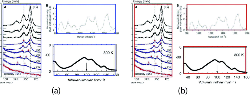 | ||
| Fig. 2 Examples of axis misalignment. (a) There are noticeable gaps between the left/bottom edges of the bounding boxes (blue boxes) and the axes. (b) The left/bottom edges of the bounding boxes (red boxes) are perfectly aligned with the axes. Figures are from ref. 6–8 (left to right, top to down). | ||
The first term forces the left edge to have constant values and the second term forces the bottom edge to have constant values. Then, the axis alignment module is optimized with both the detection loss and the edge-based loss:
 | (3) |
However, the edge-based loss term is not differentiable, which means the eqn (3) cannot be optimized directly. In practice, we take the one-step Majorization–Minimization strategy to solve the problem.
 | (4) |
As shown in eqn (4), we first optimize the detection model with the gradient descent method to generate bounding boxes with high confidence scores, then we refine the left/bottom edges of the detected bounding boxes via a nearest neighbor search. In particular, we apply the probabilistic Hough transform42 to detect lines (i.e. axes candidates) in the graph image and then search for the most confident candidates. Intuitively, the best candidates should be either horizontal or vertical, long enough and close to the edges of the detected bounding box.
 | (5) |
 denotes the probabilistic Hough transform operator, E ∈ {Eleft, Ebottom} denotes the left or bottom edge of the bounding box. Dangle measures the cosine similarity between the given two lines. Dlength measures the ratio between the length of the detected line and the edge, and Ddist measures the horizontal/vertical distance between the two parallel lines. Empirically, ε1 and ε2 are set to be 0.98 and 0.5, respectively.
3.2 Plot data extraction
In the plot data extraction module, we first perform semantic segmentation to separate pixels belonging to plot lines from the background, and from there, apply optical flow constraints to the plot line pixels to assign them to the appropriate line (data instance) they encode. | (6) |
 denotes the probability map, which is computed by the semantic segmentation model S from the given plot image Ip.
  denotes the ground truth semantic map, ci is 1 if it is a foreground pixel and otherwise 0.
Pixel embedding in conventional instance segmentation is likely to fail because the plot lines often do not have a sufficient number of distinguishable features between different instances. As shown in Fig. 4, all pixels belonging to a single line (data instance) should be assigned to the same color. One common mode of failure in conventional instance segmentation models (i.e. LaneNet,33 SpatialEmbedding37) involves assigning multiple colors to pixels within a single line. Another common failure mode is a result of misclassifications of the pixels during segmentation (see second row in Fig. 4, LaneNet misclassifies background pixels as foreground and SpatialEmbedding misclassifies foreground pixels as background).
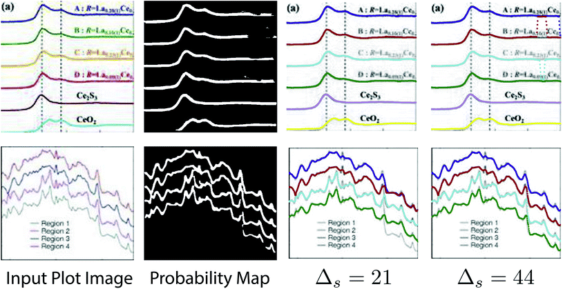 | ||
| Fig. 3 Results of plot line detection with different Δs. Too large or too small values fail to have a correct detection. Figures are from ref. 38 and 39 (top to down). | ||
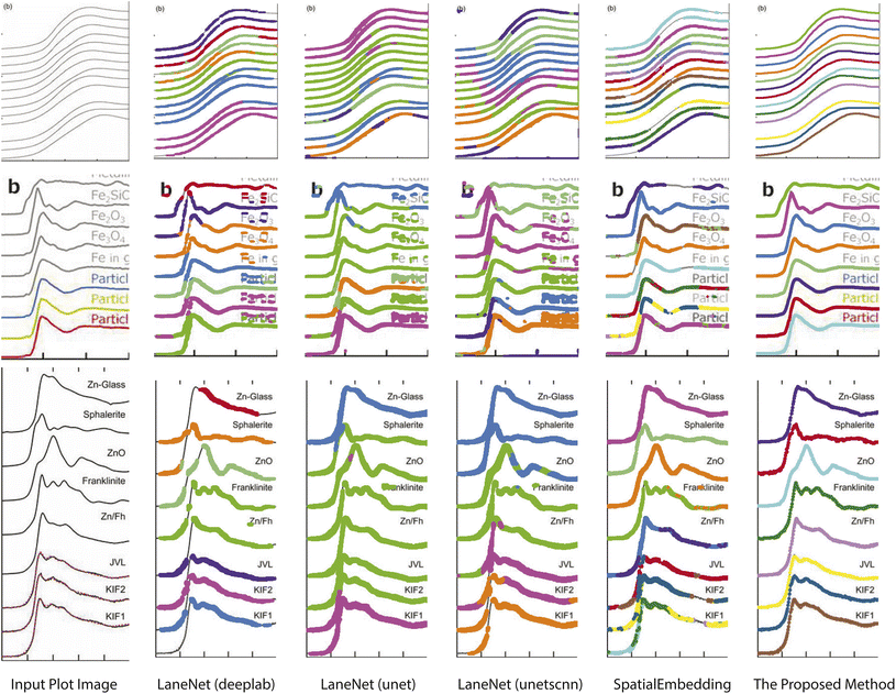 | ||
| Fig. 4 Comparison of the results of plot data extraction between instance segmentation algorithms and the proposed method. The first column is the input plot images and the rest columns are plot line detection results with different methods. All pixels belonging to a single line (data instance) should be assigned to the same color. Figures are from from ref. 1, 43 and 44 (top to down). | ||
Intuitively, plot lines are made of a set of pixels of the same value and have some statistical properties, such as smoothness and continuity. Here, we formulate the plot line detection problem as tracking the trace of a single point moving towards the y axis direction as the value of x increases. In particular, we introduce an optical flow based method to solve this tracking problem.
| Ip(x, y) = Ip(x + dx, y + dy) | (7) |
Brightness constancy, a basic assumption of optical flow, requires the intensity of the object to remain constant while in motion, as shown in eqn (7). Based on this property, we introduce the intensity constraint to force the intensity of pixels to be constant along the line.
 | (8) |
Then we apply a first order Taylor expansion to eqn (7), which estimates the velocity of the point towards y axis direction at different positions. Based on this, we introduce the smoothness constraint to force the plot line to be differentiable everywhere, i.e.
 | (9) |
Also, we introduce the semantic constraint to compensate the optical flow estimation and force more foreground pixels to fall into the plot line.
 | (10) |
Therefore, the total loss for plot line detection is
 | (11) |
4 Experiments
In this section, we conduct extensive experiments to validate the effectiveness and superiority of the proposed method.We collected a large number of graph images from literature using the EXSCLAIM! pipeline50,51 with the keyword “Raman” and “XANES”. Then we randomly selected 1800 images for the axis alignment task, with 800 images for training and 1000 images for validation. For the plot data extraction task, we labeled 336/223 plot images as the training/testing set with LabelMe.52 One thing to clarify here is that these real collected plot images may look “in low quality”, as shown in Fig. 4–6.
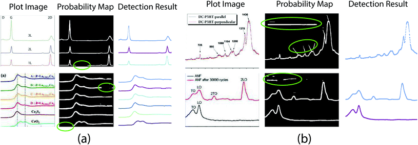 | ||
| Fig. 5 Plot line detection with imperfect semantic segmentation results. (a) Part of plot lines is missing in the probability map. Figures are from ref. 38 and 45 (top to bottom). (b). Background pixels are misclassified as foreground. Figures are from ref. 46 and 47 (top to bottom). | ||
 | ||
| Fig. 6 Plot line detection with hard examples. The proposed method works for cases containing significant overlap between different plot lines –conditions that can even be challenging for humans to annotate or disambiguate. Figures are from ref. 48 and 49 (left to right). | ||
During the training process, we implement all baseline object detection models14,15,17 with the MMDetection codebase.53 The re-implementations strictly follow the default settings of MMDetection. All models are initialized with pre-trained weights on the MS-coco dataset and then fine tuned with SGD optimizer with the labeled dataset for 1000 epochs in total, with initial learning rate as 0.005. Weight decay and momentum are set as 0.0001 and 0.9, respectively. We train the semantic segmentation module from37 in a semi-supervised manner. In particular, we simulate plot images with variations on the number/shape/color/width of plot lines, with/without random noise/blur and then we train the model alternatively with the simulated data and real labeled data for 1000 epochs.
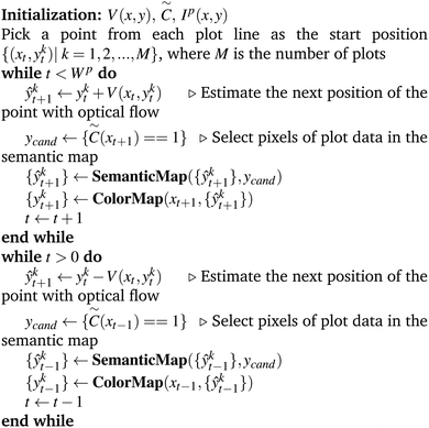
The optical flow based method is implemented in Algorithm 1.
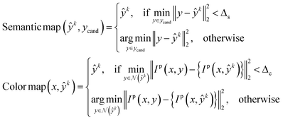 | (12) |
 denotes the neighborhood of y, all values in the interval between y − δ and y + δ. Empirically, δ is 10 in this paper. Δs, Δc are two thresholds, which help to suppress imperfection in the probability map (e.g. reject misclassified background pixels and inpaint missing foreground pixels). It is important to note that a proper value for Δs is important for doing a successful plot line detection. As shown in Fig. 3, if the Δs is too large (top row), the proposed method fails to inpaint correct misclassified foreground pixels, if the Δs is too small, the proposed method fails to compensate the error from optical flow estimation in case of sudden gradient change (e.g. peak).
Visual comparison on plot line detection between the proposed method and conventional instance segmentation algorithms is shown in Fig. 4. In particular, we have 4 baseline methods: LaneNet33 with Deeplab54 as the backbone, LaneNet with Unet55 as the backbone, LaneNet with Unetscnn56 as the backbone and SpatialEmbedding.37 All the instance segmentation algorithms fail to distinguish pixels from different plot lines especially when the number of lines increases and the distance between adjacent lines decreases (e.g. first row in Fig. 4). As expected, the proposed optical flow based method correctly groups pixels into plot lines. Moreover, the proposed method still works even with imperfect semantic segmentation prediction. As shown in Fig. 5, the proposed method is able to inpaint the missing pixels and eliminate misclassified background pixels. The proposed plot line detection method also works for cases containing significant overlap between different plot lines – conditions that can even be challenging for humans to annotate or disambiguate. This is shown in Fig. 6.
Meanwhile, we introduce a quantitative metric to evaluate the performance of different methods. Here, {Lpred} and {Lgt} denote the set of detected plot lines and ground truth plot lines in the image, respectively. Then we define matched plot lines as  while each ground truth plot line can have at most one matched plot line. Thus we have
  where ‖.‖ denotes the number of plot lines in the set and εp denotes the threshold of the mean absolute pixel distance between two plot lines. By setting different εp, we measure the performance of different algorithms, as shown in Fig. 7. As expected, the proposed algorithm achieves better precision and recall accuracy than the other methods. In particular, there are 935 plot lines in the testing set. Given εp = 1, the proposed plot digitizer detects 831 matched plot lines and given εp = 2, the proposed plot digitizer detects 890 matched plot lines.
5 Ablation study
5.1 Edge-based constraint
We introduce a mean absolute distance between the estimated axes and the real axes to quantitatively measure the axis misalignment. Here we use (xpred, ypred) and (xgt, ygt) to denote the estimated and ground truth point of origin of the coordinates, respectively. Then the axis misalignment is computed as | (13) |
We measure the axis misalignment of the detection results using three different anchor-free object detection models (i.e. FCOS,14 FreeAnchor17 and GuidedAnchor15), with and without the edge-based constraint. A more detailed quantitative comparison between axis alignment with/without the edge-based constraint is shown in Table 2. The refinement with the edge-based constraint suppresses the axis misalignment, with ∼10% improvement for FCOS and ∼47% improvement for the other detectors.
5.2 Different losses for plot line detection
We conduct experiments to study how each loss term affects performance of the plot data extraction module. A visual comparison between plot data extraction with different loss function is shown in Fig. 8. We take an example plot image from the testing set. With only the smoothness loss (i.e. middle left image), the extraction process is significantly affected by the imperfection of the plot image (e.g. noise), which produces an inaccurate gradient map. Adding the semantic loss term helps to compensate for the errors in the optical flow estimation, which results in significant improvements (i.e. middle right image). However, some glitches are still noticeable in the detection result (i.e. the green plot in middle right image). Finally, the intensity constraint term helps refine the detection results (i.e. right most image) by searching for the best intensity match in the neighborhood.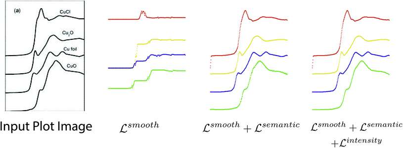 | ||
| Fig. 8 Visual comparison of plot data extraction with different losses. The leftmost figure is the input plot image. With only the smoothness loss (i.e. middle left image), the extraction process is significantly affected by the imperfection of the plot image (e.g. noise), which produces an inaccurate gradient map. With both the smoothness loss and the semantic loss (i.e. middle right image), the semantic loss term helps to compensate for the errors in the optical flow estimation, which results in significant improvements. With the smoothness loss, the semantic loss and the intensity constraint (i.e. right most image), the intensity constraint term helps refine the detection results by searching for the best intensity match in the neighborhood, which eliminates the glitches. Figure is from ref. 57. | ||
5.3 Different start positions for plot line detection
A good start position matters in the proposed optical flow method, especially in case that there are sharp peaks in the plot image or misclassified foreground/background pixels in the probability map. Intuitively, we select the start position at places where the gradients are small. As shown in Fig. 9, the top row shows that misclassified foreground pixels break the continuity of the plot line, which hinders the ability of tracking the motion of the point from one side. In the bottom row, there are sharp peaks in the plot image and significant overlap between different plot lines in the probability map, making it difficult to apply the optical flow method from the left side of the peak. Also, we conduct experiments to quantitatively measure the how the selection of start positions affect the performance. In particular, we randomly select ∼20 start positions in each plot image and apply the proposed method to detect plot lines. We measure the best/average/worst performance of plot line detection with these start positions, as shown in Fig. 10. Clearly, selecting a proper start position is very important to the success of the algorithm.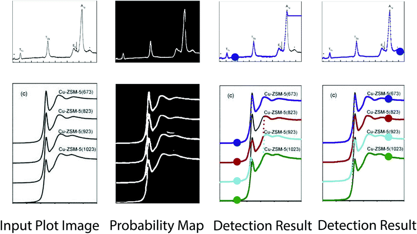 | ||
| Fig. 9 Results of plot line detection with different start position. Start positions are highlighted in the detection result images. Figures are from ref. 57 and 58 (top to down). | ||
5.4 Different line width and line style for plot line detection
Different authors may prefer different line width or line styles when they generate the plot images. We conduct experiments to study how the variation of line width and line styles in the plot images would affect the proposed plot line detection model. For quantitative evaluation, we take 200 spectra from the benchmark database.† We generate a number of plot images with different line widths and line styles. In particular, solid lines, dashed lines, dashed-dot lines and dotted lines are commonly used and the line width is randomly selected from {2.0, 2.5, 3.0, 4.0}. Fig. 11(a) shows an example of the synthetic plot images, in which different plot lines have different line styles and colors. Since the semantic segmentation module is trained with both simulated data and real labeled data, we directly apply the trained model onto those synthetic plot images for plot line detection. As expected, the model works pretty well on the synthetic data. As shown in Fig. 11(b), each plot line is assigned with one unique color. Moreover, we noticed that the data range of different plot lines could be different, then we generate the confidence map for each predicted plot line, as shown in Fig. 11(c), where data points in red are likely to be false positive prediction and data points in green are likely to be true positive prediction.In this experiment, 195 out of 200 plot lines are detected, resulting a recall ratio of 97.5%. Then we compute the root mean square error (RMSE) between the predicted spectra data and the ground truth data with different line width or line styles. In particular, the predicted spectra data and the ground truth data of each plot line are normalized to [0, 1]. Also, since the coordinates of the predicted spectra data are integer while the ground truth data can be floating numbers, a bilinear interpolation is applied to align the prediction and the ground truth data. In total, the average RMSE of all detected plot lines is 0.018. We also compute the average RMSE for different settings of line width or line styles, as shown in Table 3. As expected, the RMSE of solid plot lines is better than that of plot lines in other line styles since solid lines are the most widely used line style. The proposed model also performs quite robust in case of different line width and line styles.
| Line width | RMSE | Line style | RMSE |
|---|---|---|---|
| 2.0 | 0.015 | Solid | 0.009 |
| 2.5 | 0.023 | Dashed | 0.022 |
| 3.0 | 0.016 | Dashed-dot | 0.016 |
| 4.0 | 0.018 | Dotted | 0.026 |
6 Conclusion and discussion
In this paper, we report the Plot2Spectra code we developed to extract data points from XANES/Raman spectroscopy images and transform them into coordinates, which enables large scale data collection, analysis, and machine learning of these types of spectroscopy data. The novelty of the technique is that we propose a hybrid system to address the problem. Due to the insufficient feature of plot lines, it is difficult for conventional instance segmentation methods to find a proper embedding space. To this end, we decouple the problem into an easy-to-model part (i.e. optical flow for data point tracking) and a hard-to-model part (i.e. CNN for plot data segmentation). Extensive experiments validate the effectiveness and superiority of the proposed method compared to other approaches, even for very challenging examples.Unfortunately, there remain some cases that the proposed approach is likely to fail. As shown in Fig. 12(a), the current model fails to detect sharp peaks. This is because the first order Taylor approximation in eqn (9) does not hold for large displacements. A possible way to address this issue is to stretch the plot image along x-direction, which reduces the slope of the peaks. Another kind of failure cases is shown in Fig. 12(b). Since the proposed plot line detection algorithm detects plot lines in a sequential manner, the error from the previous stage (i.e. semantic segmentation) would affect the performance of the subsequent stage (i.e. optical flow based method). Even though the optical flow based method is robust if some pixels are misclassified (as shown in Fig. 5), significant errors in the probability map would still result in a failure. A possible way to address this issue could be training a more advanced semantic segmentation model with more labeled data.
 | ||
| Fig. 12 Failure cases. (a) Plot2Spectra fails when there is a significant peak. Figures are from ref. 65 and 66 (top to down). (b) Plot2Spectra fails when a large portion of background/foreground pixels are misclassified. Figures are from ref. 67 and 68 (top to down). | ||
Data availability
(1) The code described in this paper can be found at https://github.com/MaterialEyes/Plot2Spec. The version of the code employed for this study is version 1.0. (2) Data and processing scripts for this paper, including plot images used in the training, are available at https://github.com/MaterialEyes/Plot2Spec.Author contributions
The authors confirm contribution to the paper as follows: study conception and design: Weixin Jiang, Maria K. Y. Chan; data collection: Weixin Jiang, Trevor Spreadbury, Maria K. Y. Chan; analysis and interpretation of results: Weixin Jiang, Eric Schwenker, Kai Li, Maria K. Y. Chan, Oliver Cossairt; draft manuscript preparation: Weixin Jiang. All authors reviewed the results and approved the final version of the manuscript.Conflicts of interest
There are no conflicts to declare.Acknowledgements
We thank Yiming Chen for assistance in obtaining spectroscopy data from the Materials Project. MKYC and WJ acknowledge the support from the BES SUFD Early Career award. Work at Argonne and Northwestern is based, in part, upon work supported by Laboratory Directed Research and Development (LDRD) funding from Argonne National Laboratory, provided by the Director, Office of Science, of the U.S. Department of Energy under Contract No. DE-AC02-06CH11357. Work performed at the Center for Nanoscale Materials, a U.S. Department of Energy Office of Science User Facility, was supported by the U.S. DOE, Office of Basic Energy Sciences, under Contract No. DE-AC02-06CH11357. WJ, ES, and TS gratefully acknowledge the computing resources provided and operated by the Joint Laboratory for System Evaluation (JLSE) at Argonne National Laboratory.Notes and references
- N. Rivera, D. Hesterberg, N. Kaur and O. W. Duckworth, Energy Fuels, 2017, 31, 9652–9659 CrossRef CAS.
- S. Kataria, W. Browuer, P. Mitra and C. L. Giles, AAAI, 2008, 1169–1174 Search PubMed.
- J. Luo, Z. Li, J. Wang and C.-Y. Lin, Proceedings of the IEEE/CVF Winter Conference on Applications of Computer Vision, 2021, pp. 1917–1925 Search PubMed.
- X. Lu, S. Kataria, W. J. Brouwer, J. Z. Wang, P. Mitra and C. L. Giles, International Journal on Document Analysis and Recognition (IJDAR), 2009, 12, 65–81 CrossRef.
- A. Rohatgi, Webplotdigitizer: Version 4.4, 2020, https://automeris.io/WebPlotDigitizer Search PubMed.
- E. Saitoh, S. Okamoto, K. Takahashi, K. Tobe, K. Yamamoto, T. Kimura, S. Ishihara, S. Maekawa and Y. Tokura, Nature, 2001, 410, 180–183 CrossRef CAS PubMed.
- S. Teh, W. Zheng, K. Ho, M. Teh, K. Yeoh and Z. Huang, Br. J. Cancer, 2008, 98, 457–465 CrossRef CAS PubMed.
- A. Sirenko, C. Bernhard, A. Golnik, A. M. Clark, J. Hao, W. Si and X. Xi, Nature, 2000, 404, 373–376 CrossRef PubMed.
- S. Ren, K. He, R. Girshick and J. Sun, arXiv preprint arXiv:1506.01497, 2015.
- J. Redmon and A. Farhadi, Proceedings of the IEEE conference on computer vision and pattern recognition, 2017, pp. 7263–7271 Search PubMed.
- J. Redmon and A. Farhadi, arXiv preprint arXiv:1804.02767, 2018.
- J. Redmon, S. Divvala, R. Girshick and A. Farhadi, Proceedings of the IEEE conference on computer vision and pattern recognition, 2016, pp. 779–788 Search PubMed.
- X. Zhou, C. Yao, H. Wen, Y. Wang, S. Zhou, W. He and J. Liang, Proceedings of the IEEE conference on Computer Vision and Pattern Recognition, 2017, pp. 5551–5560 Search PubMed.
- Z. Tian, C. Shen, H. Chen and T. He, Proceedings of the IEEE/CVF International Conference on Computer Vision, 2019, pp. 9627–9636 Search PubMed.
- J. Wang, K. Chen, S. Yang, C. C. Loy and D. Lin, Proceedings of the IEEE/CVF Conference on Computer Vision and Pattern Recognition, 2019, pp. 2965–2974 Search PubMed.
- T. Yang, X. Zhang, Z. Li, W. Zhang and J. Sun, arXiv preprint arXiv:1807.00980, 2018.
- X. Zhang, F. Wan, C. Liu, X. Ji and Q. Ye, IEEE Transactions on Pattern Analysis and Machine Intelligence, 2021 Search PubMed.
- J. Long, E. Shelhamer and T. Darrell, Proceedings of the IEEE conference on computer vision and pattern recognition, 2015, pp. 3431–3440 Search PubMed.
- Y. Liu and L. Jin, Proceedings of the IEEE Conference on Computer Vision and Pattern Recognition, 2017, pp. 1962–1969 Search PubMed.
- M. Liao, Z. Zhu, B. Shi, G.-s. Xia and X. Bai, Proceedings of the IEEE conference on computer vision and pattern recognition, 2018, pp. 5909–5918 Search PubMed.
- Y. Zhou, Q. Ye, Q. Qiu and J. Jiao, Proceedings of the IEEE Conference on Computer Vision and Pattern Recognition, 2017, pp. 519–528 Search PubMed.
- B. Shi, X. Bai and S. Belongie, Proceedings of the IEEE conference on computer vision and pattern recognition, 2017, pp. 2550–2558 Search PubMed.
- Y. Baek, B. Lee, D. Han, S. Yun and H. Lee, Proceedings of the IEEE/CVF Conference on Computer Vision and Pattern Recognition, 2019, pp. 9365–9374 Search PubMed.
- M. Jaderberg, K. Simonyan, A. Zisserman and K. Kavukcuoglu, arXiv preprint arXiv:1506.02025, 2015.
- K. He, X. Zhang, S. Ren and J. Sun, Proceedings of the IEEE conference on computer vision and pattern recognition, 2016, pp. 770–778 Search PubMed.
- K. Simonyan and A. Zisserman, arXiv preprint arXiv:1409.1556, 2014.
- B. Shi, X. Bai and C. Yao, IEEE transactions on pattern analysis and machine intelligence, 2016, 39, 2298–2304 Search PubMed.
- B. Shi, X. Wang, P. Lyu, C. Yao and X. Bai, Proceedings of the IEEE conference on computer vision and pattern recognition, 2016, pp. 4168–4176 Search PubMed.
- Z. Cheng, F. Bai, Y. Xu, G. Zheng, S. Pu and S. Zhou, Proceedings of the IEEE international conference on computer vision, 2017, pp. 5076–5084 Search PubMed.
- J. Baek, G. Kim, J. Lee, S. Park, D. Han, S. Yun, S. J. Oh and H. Lee, Proceedings of the IEEE/CVF International Conference on Computer Vision, 2019, pp. 4715–4723 Search PubMed.
- K. He, G. Gkioxari, P. Dollár and R. Girshick, Proceedings of the IEEE international conference on computer vision, 2017, pp. 2961–2969 Search PubMed.
- S. Liu, L. Qi, H. Qin, J. Shi and J. Jia, Proceedings of the IEEE conference on computer vision and pattern recognition, 2018, pp. 8759–8768 Search PubMed.
- D. Neven, B. De Brabandere, S. Georgoulis, M. Proesmans and L. Van Gool, 2018 IEEE intelligent vehicles symposium (IV), 2018, pp. 286–291 Search PubMed.
- B. De Brabandere, D. Neven and L. Van Gool, arXiv preprint arXiv:1708.02551, 2017.
- S. Kong and C. C. Fowlkes, Proceedings of the IEEE Conference on Computer Vision and Pattern Recognition, 2018, pp. 9018–9028 Search PubMed.
- A. Newell, Z. Huang and J. Deng, arXiv preprint arXiv:1611.05424, 2016.
- D. Neven, B. D. Brabandere, M. Proesmans and L. V. Gool, Proceedings of the IEEE/CVF Conference on Computer Vision and Pattern Recognition, 2019, pp. 8837–8845 Search PubMed.
- Y. Fujita, K. Kinami, Y. Hanada, M. Nagao, A. Miura, S. Hirai, Y. Maruyama, S. Watauchi, Y. Takano and I. Tanaka, ACS Omega, 2020, 5, 16819–16825 CrossRef CAS PubMed.
- G. Shetty, C. Kendall, N. Shepherd, N. Stone and H. Barr, Br. J. Cancer, 2006, 94, 1460–1464 CrossRef CAS.
- T.-Y. Lin, P. Goyal, R. Girshick, K. He and P. Dollár, Proceedings of the IEEE international conference on computer vision, 2017, pp. 2980–2988 Search PubMed.
- J. Yu, Y. Jiang, Z. Wang, Z. Cao and T. Huang, Proceedings of the 24th ACM international conference on Multimedia, 2016, pp. 516–520 Search PubMed.
- N. Kiryati, Y. Eldar and A. M. Bruckstein, Pattern Recognition, 1991, 24, 303–316 CrossRef.
- S. Hinokuma, Y. Kawabata, S. Matsuki, H. Shimanoe, S. Kiritoshi and M. Machida, J. Phys. Chem. C, 2017, 121, 4188–4196 CrossRef CAS.
- Y. Abe, Y. Iizawa, Y. Terada, K. Adachi, Y. Igarashi and I. Nakai, Anal. Chem., 2014, 86, 8521–8525 CrossRef CAS PubMed.
- R. W. Havener, A. W. Tsen, H. C. Choi and J. Park, NPG Asia Mater., 2011, 3, 91–99 CrossRef.
- S. Qu, Q. Yao, L. Wang, Z. Chen, K. Xu, H. Zeng, W. Shi, T. Zhang, C. Uher and L. Chen, NPG Asia Mater., 2016, 8, e292 CrossRef CAS.
- M. Yu, W. Wang, C. Li, T. Zhai, X. Lu and Y. Tong, NPG Asia Mater., 2014, 6, e129 CrossRef CAS.
- J. Xu, A. P. Wilkinson and S. Pattanaik, Chem. Mater., 2000, 12, 3321–3330 CrossRef CAS.
- A. L. Dadlani, S. Acharya, O. Trejo, F. B. Prinz and J. Torgersen, ACS Appl. Mater. Interfaces, 2016, 8, 14323–14327 CrossRef CAS PubMed.
- W. Jiang, E. Schwenker, T. Spreadbury, N. Ferrier, M. K. Chan and O. Cossairt, arXiv preprint arXiv:2101.09903, 2021.
- E. Schwenker, W. Jiang, T. Spreadbury, N. Ferrier, O. Cossairt and M. K. Chan, arXiv preprint arXiv:2103.10631, 2021.
- K. Wada, labelme: Image Polygonal Annotation with Python, 2016, https://github.com/wkentaro/labelme Search PubMed.
- K. Chen, J. Wang, J. Pang, Y. Cao, Y. Xiong, X. Li, S. Sun, W. Feng, Z. Liu, J. Xu, Z. Zhang, D. Cheng, C. Zhu, T. Cheng, Q. Zhao, B. Li, X. Lu, R. Zhu, Y. Wu, J. Dai, J. Wang, J. Shi, W. Ouyang, C. C. Loy and D. Lin, MMDetection: Open MMLab Detection Toolbox and Benchmark, 2019 Search PubMed.
- L.-C. Chen, G. Papandreou, I. Kokkinos, K. Murphy and A. L. Yuille, DeepLab: Semantic Image Segmentation with Deep Convolutional Nets, Atrous Convolution, and Fully Connected CRFs, 2017 Search PubMed.
- O. Ronneberger, P. Fischer and T. Brox, U-Net: Convolutional Networks for Biomedical Image Segmentation, 2015 Search PubMed.
- X. Pan, J. Shi, P. Luo, X. Wang and X. Tang, Spatial As Deep: Spatial CNN for Traffic Scene Understanding, 2017 Search PubMed.
- Y. Zhang, I. J. Drake and A. T. Bell, Chem. Mater., 2006, 18, 2347–2356 CrossRef CAS.
- J. Xu, G. Hou, H. Li, T. Zhai, B. Dong, H. Yan, Y. Wang, B. Yu, Y. Bando and D. Golberg, NPG Asia Mater., 2013, 5, e53 CrossRef CAS.
- K. Mathew, C. Zheng, D. Winston, C. Chen, A. Dozier, J. J. Rehr, S. P. Ong and K. A. Persson, Sci. Data, 2018, 5, 1–8 CrossRef PubMed.
- Y. Chen, C. Chen, C. Zheng, S. Dwaraknath, M. K. Horton, J. Cabana, J. Rehr, J. Vinson, A. Dozier and J. J. Kas, Sci. Data, 2021, 8, 1–8 CAS.
- A. Jain, S. P. Ong, G. Hautier, W. Chen, W. D. Richards, S. Dacek, S. Cholia, D. Gunter, D. Skinner and G. Ceder, APL Mater., 2013, 1, 011002 CrossRef.
- C. Zheng, K. Mathew, C. Chen, Y. Chen, H. Tang, A. Dozier, J. J. Kas, F. D. Vila, J. J. Rehr and L. F. Piper, npj Comput. Mater., 2018, 4, 1–9 CrossRef CAS.
- S. B. Torrisi, M. R. Carbone, B. A. Rohr, J. H. Montoya, Y. Ha, J. Yano, S. K. Suram and L. Hung, npj Comput. Mater., 2020, 6, 1–11 CrossRef.
- M. R. Carbone, S. Yoo, M. Topsakal and D. Lu, Phys. Rev. Mater., 2019, 3, 033604 CrossRef CAS.
- F. Liu, J. Huang, K. Sun, C. Yan, Y. Shen, J. Park, A. Pu, F. Zhou, X. Liu and J. A. Stride, NPG Asia Mater., 2017, 9, e401 CrossRef CAS.
- R. Baker, K. Rogers, N. Shepherd and N. Stone, Br. J. Cancer, 2010, 103, 1034–1039 CrossRef CAS PubMed.
- H. Daniel, A. M. Gholami, D. Berry, C. Desmarchelier, H. Hahne, G. Loh, S. Mondot, P. Lepage, M. Rothballer and A. Walker, ISME J., 2014, 8, 295–308 CrossRef CAS PubMed.
- R. U. Chandrasena, W. Yang, Q. Lei, M. U. Delgado-Jaime, K. D. Wijesekara, M. Golalikhani, B. A. Davidson, E. Arenholz, K. Kobayashi and M. Kobata, Nano Lett., 2017, 17, 794–799 CrossRef CAS PubMed.
Footnote |
† The XASdb59,60 hosted on the Materials Project61 website, currently the world's largest database for computed X-ray absorption spectroscopy (XAS) data. This database stores more than 500![[thin space (1/6-em)]](https://www.rsc.org/images/entities/char_2009.gif) 000 site-wise spectra and has been extensively used to accelerate the spectra interpretation through machine learning approaches.62–64 000 site-wise spectra and has been extensively used to accelerate the spectra interpretation through machine learning approaches.62–64 |
| This journal is © The Royal Society of Chemistry 2022 |

