Velocity map imaging with no spherical aberrations†
Received
2nd August 2023
, Accepted 24th August 2023
First published on 28th August 2023
Abstract
Velocity map imaging (VMI) is a powerful technique to deduce the kinetic energy of ions or electrons that are produced from a large volume in space with good resolution. The size of the acceptance volume is determined by the spherical aberrations of the ion optical system. Here we present an analytical derivation for velocity map imaging with no spherical aberrations. We will discuss a particular example for the implementation of the technique that allows using the reaction microscope recently installed in the cryogenic storage ring (CSR) in a VMI mode. SIMION simulations confirm that a beam of electrons produced almost over the entire volume of the source region, with a width of 8 cm, can be focused to a spot of 0.1 mm on the detector. The use of the same formalism for position imaging, as well as in a mixed mode where position imaging is in one axis and velocity map imaging is in a different axis, is also discussed.
1 Introduction
The objective of photo-electron spectroscopy (PES) is to determine the energy of the atomic/molecular orbitals,1,2 along with their symmetry3,4 and excited state dynamics by measuring the velocity components of photo-emitted electrons.5 In imaging applications using PES, this is achieved by accelerating the electrons towards a position-sensitive particle detector and measuring their 2-dimensional impact positions and, if possible, also their time-of-flight (TOF).6,7 A similar approach is used in ion imaging to understand the kinetic energy release of ions produced in gas phase reactions.8 In these imaging measurements the three measured quantities (the time-of-flight and the impact positions on the detector) depend on the important 6 parameters: the three components of the particle's initial velocity, and the three components of the particle's position of origin (which in this case are not of interest). There are two main strategies for avoiding the broadening of the measured spectra due to the uncertainty in the particle's source point. The first is to create electrons/ions from a small region in space, for example by tightly focusing a photo-ionizing laser. The second approach, known as velocity map imaging (VMI, also known as ‘position focusing’), which was first described by Eppink and Parker in 1997,9 is to use electrostatic focusing to ensure that the impact position on the detector does not depend on the particle's original position but only on the particle's initial velocity. An intuitive understanding of this approach builds on the equivalence between optics and ion optics. In optics, when the detector is positioned in the focal plane of the lens (also known as the Fourier plane) parallel rays of light are focused to a point, i.e., the impact position does not depend on the size or extension of the light source but only on its directionality. Correspondingly, in ion optics, VMI is achieved using an electrostatic lens whose voltage is set so that its focal plane lies on the detector. Notably, the technical constraints in ion optics are different. Here, the main constraint is that the electric potential, V(x,y,z), must satisfy the Laplace equation:| | 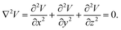 | (1) |
In practice, the design of ion optical devices usually adds additional constraints. For example, one would like to use only a small number of electrodes and power supplies. Most VMI designs use a large field free region, or a region with a constant electric field.10 The original work by Eppink and Parker9 employed only three electrodes (a repeller, an extractor and a ground electrode); however, it soon became clear that one can reduce spherical aberrations by adding more electrodes.8 A comprehensive review of the different implementations of VMI is beyond the scope of this paper; we will only note that configurations with a large number of electrodes spanning the entire volume from the interaction region to the detector (known as ‘thick lens’ designs) are increasingly being used.10–16 However, as the complexity increases, finding the optimal design and voltages becomes more challenging requiring extensive iterative simulations.13 According to a recent work,15 the current state of the art enables focusing a beam with a width of a few mm in the on-source region to a ≃0.1 mm spot on the detector, resulting in a ‘focusing factor’ (also known as a ‘blurring factor’) of ≃0.05.15
In the following we will analyze charged particle trajectories in a quadratic electrostatic potential and demonstrate how it can be used for VMI with no spherical aberrations. We discuss the practical implementation of this methodology as a method for implementing photoelectron spectroscopy in the Cryogenic Storage Ring (CSR), located at the Max Planck Institute for Nuclear Physics (MPIK), Heidelberg, Germany. The CSR is a purely electrostatic ion storage ring with a circumference of 35 m, which can be cooled down to a few degrees kelvin. The primary goal of the CSR is to study laboratory astrophysics as for the storage of ions in conditions of extremely low pressure and cryogenic temperature similar to the conditions in the interstellar medium, and to study astrophysically relevant reactions including the interaction of cold molecular ions with photons, electrons and neutral atoms.17
Recently, a reaction microscope (CSR-ReMi) was installed in one of the straight sections of the CSR. Reaction microscopes (also known as COLTRIMS) use a combination of electric and magnetic fields and two opposing particle detectors to image, in coincidence, both electrons and charged fragments resulting from chemical reactions. Consequently, the kinetic energy of the electrons, as well as the mass and kinetic energy of the charged fragments is determined, resulting in a full kinematic description of the reaction.18–20 We present below SIMION simulations21 of how the CSR-ReMi can be operated in a VMI mode. We show that using the analytically derived voltages, with no further optimization, one can focus electrons from most of the inner diameter of the electrodes down to a spot size smaller than the spatial resolution of the detector, resulting in a focusing factor that is 40 times smaller than the current state-of-the-art value.15 In addition, we discuss how the same methodology can be used for position imaging and in a mixed mode in which there is position imaging along one axis and velocity map imaging along the other axis.
2 VMI with a quadratic electric potential
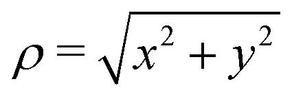
Let us denote the main axis of the spectrometers (i.e. the direction from the interaction point to the middle of the detector) as the ẑ direction, and the ![[x with combining circumflex]](https://www.rsc.org/images/entities/i_char_0078_0302.gif) , ŷ plane as the ‘transverse plane’. Examine the following quadratic solution of the Laplace equation (eqn (1)):
, ŷ plane as the ‘transverse plane’. Examine the following quadratic solution of the Laplace equation (eqn (1)):| | | V(ρ,z) = Uρ(ρ2 − 2z2) − Uzz | (2) |
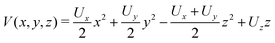
where V is the electrostatic potential,  , and Uρ and Uz are constants.
The equation of motion along the spectrometer's main axis for a particle with charge q and mass m is given by:
| | 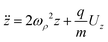 | (3) |
with the solution:
| |  | (4) |
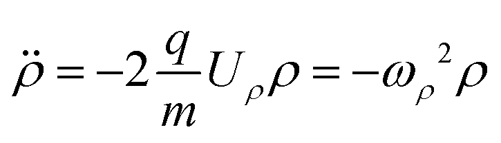
Here z0 and v0z are the initial position and velocity along the ẑ axis, respectively. The time-of-flight, tf, is set by z(tf) = L, where L is the distance to the detector. The equation of motion in the transverse direction is:
| | 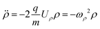 | (5) |
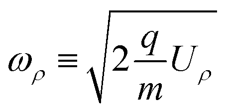
where:
| |  | (6) |
with the solution:
| | 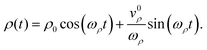 | (7) |
Here
ρ0 and
v0ρ are the initial position and velocity in the transverse direction, respectively. We denote the impact position on the detector by
ρf =
ρ(
tf). Ideal VMI conditions correspond to no dependence of
ρf on
ρ0, which is achieved by setting cos(
ωρtf) = 0, and consequently:
where
n is an integer number. We will only treat the case of
n = 0. Inserting
eqn (8) into
eqn (4), we find that the condition for VMI is:
| |  | (9) |
with:
| |  | (10) |
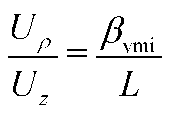
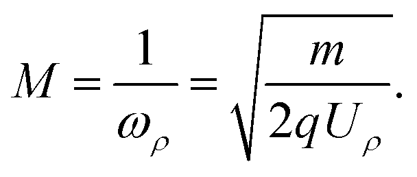
We define the magnification, M, of the device as:
| |  | (11) |
Under VMI conditions the magnification is given by:
| | 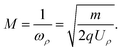 | (12) |
The two parameters
Uρ and
Uz allow us to set a desired magnification,
M, while maintaining VMI conditions. Let
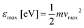
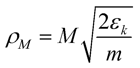
be the maximal electron kinetic energy to be measured (
i.e., an electron with this energy with velocity on the
![[small rho, Greek, circumflex]](https://www.rsc.org/images/entities/i_char_e0b7.gif)
direction only will hit the detector's radius,
Rd), then the desired magnification is given by:
| | 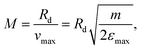 | (13) |
leading to:
| | 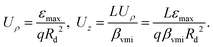 | (14) |
Due to the cylindrical symmetry, to first order the position of impact,
ρf does not depend on
z0 and
v0z. In the ESI
† the full expression for
tf is derived (
eqn (11) of the ESI
†) and is used to derive the higher order corrections for
ρf, showing that (
eqn (23) in the ESI
†):
| |  | (15) |
3 SIMION simulations of VMI imaging in the CSR-REMI
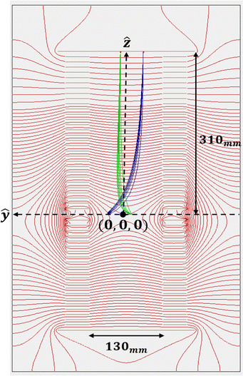
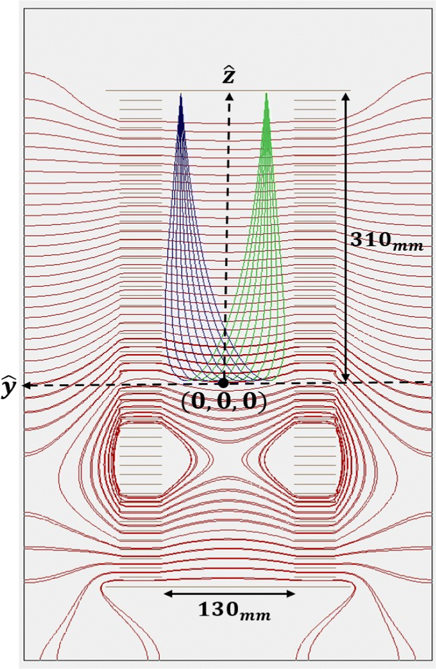
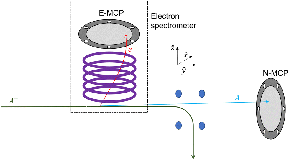
The CSR-ReMi, shown schematically in Fig. 1, consists of 51 circular concentric electrodes, each with an inner diameter of 130 mm, and microchannel plate (MCP) detectors on either side, one detector for the electrons (labeled E-MCP in Fig. 1) and one for the cationic fragments (labeled I-MCP in Fig. 1). The electrodes are connected through variable voltage dividers such that the voltage on each electrode can be set independently. The detectors have an active diameter of 120 mm and are read out using delay-line anodes with a position resolution of ≃0.16 mm. The stored ion beam will pass through the center of the ReMi where it will be intersected with a neutral gas jet or with a laser beam. The primary use of the CSR-ReMi will be dissociative ionization experiments in which the neutral molecules from the gas jet will be ionized by collisions with the stored ions. Here, we discuss the possibility of using the CSR-ReMi for performing PES of the stored ions, and to study the kinetic energy of thermionically emitted electrons. The former case refers to the possibility of irradiating the stored ion beam by laser-light within the CSR-ReMi, and imaging the photo-electrons on the E-MCP detector. In this application, due to the low ion density and because high laser intensity is not required, one would prefer not to focus the laser to a small spot but rather have a large overlap between the laser and the stored ion beam. By thermionic emission we refer to electrons emitted through delayed electron emission, i.e., electrons emitted at very long times (ranging up to milliseconds) after photon absorption, or from ions that are in highly excited states caused by their production in the ion source. In this application VMI is necessary as the electrons are not emitted from a well-defined position. The large interaction region volume we demonstrate below makes this kind of device appealing wherever a large ion source volume is required.
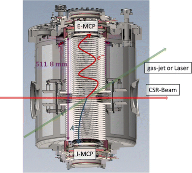 |
| | Fig. 1 A schematic illustration of the CSR-ReMi. In this illustration the stored ion beam passes through the instrument from left to right (along the direction indicated by the red arrow), and is crossed by either a neutral gas jet or by laser (along the direction indicated by the green arrow). The resulting electrons are accelerated upwards and imaged on the E-MCP detector, while the resulting cationic fragments are accelerated in the opposite direction and imaged on the I-MCP detector. | |
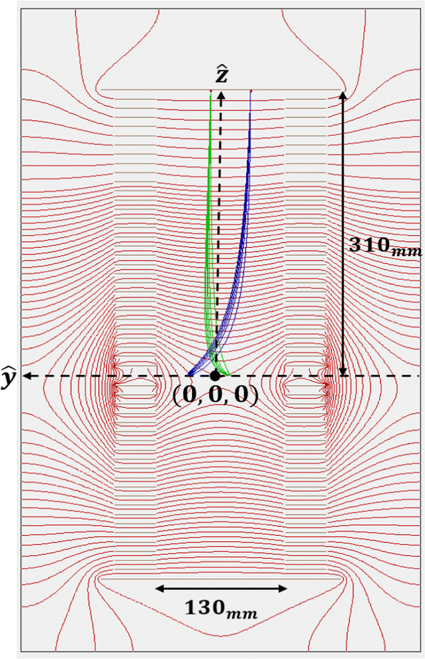
Fig. 2 shows a SIMION simulation of the CSR-ReMi in VMI mode. In the simulations we set the voltages on the electrodes according to eqn (2) (using the electrode's position and inner radius) with no further optimization. Choosing a value of εmax = 1.8 eV (which determines the values of Uρ and Uz that satisfies VMI conditions according to eqn (14)) leads to the equipotential lines shown in red in Fig. 2. As can be seen, the potential has a saddle point located at about 80 mm below the interaction region. The calculated trajectories for two monoenergetic electron beams are also shown. Here each electron beam has a width of 80 mm along the y axis, and both beams are focused to a spot size of less than 0.1 mm (corresponding to a focusing factor of 0.0125), i.e., smaller than the position resolution of the detector.
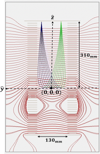 |
| | Fig. 2 A SIMION simulation of the CSR-ReMi, with equipotential lines marked in red. Also shown are electron trajectories. The blue trajectories correspond to a beam of electrons with a width of 80 mm in the ŷ direction and with a kinetic energy of 0.9 eV in the ŷ direction. The green trajectories correspond to a kinetic energy of 0.6 eV in the −ŷ direction. Both beams are focused to a spot size smaller than the position resolution of the detector (92 μm and 85 μm in diameter, respectively). | |
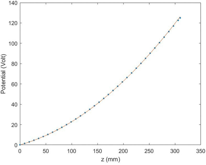
The fact that the final spot size on the detector has a width shows that there is a difference between the simulated and the analytical potentials, stemming from the finite size of the electrodes and from the fact that the detector is flat (and not in the shape of an equipotential line). However, the deviations from the analytical potential are small as can be seen in Fig. 3, where a comparison of the calculated and analytical potential is shown. In the following we present the characterization of the CSR-ReMi in VMI mode exhibiting good match between the SIMION calculations and the analytical derivation.
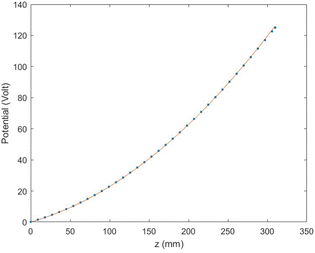 |
| | Fig. 3 Comparison of the numerically calculated potential along the ẑ axis (for the same value of εmax used in Fig. 2), as a function of z, to the analytical formula (eqn (2)). Here z = 0 corresponds to the center of the interaction zone. We observe small deviations (up to 1.2%) from the analytical potential only at small distances (<15 mm) from the detector. | |
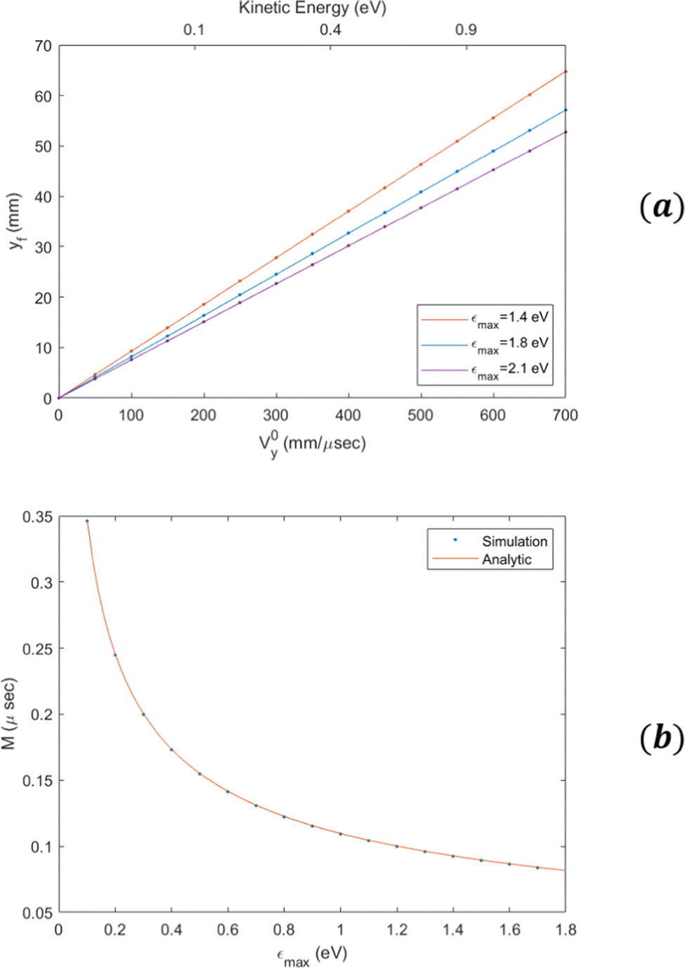
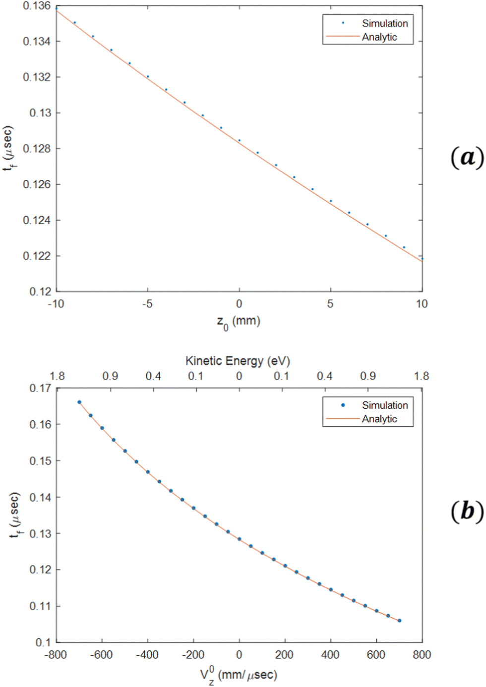
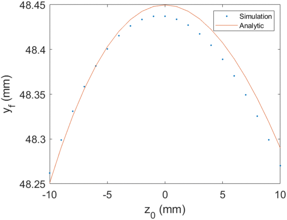
Fig. 4(a) shows yf as a function of v0y, for several different values of εmax. As expected, we observe a linear dependence of the impact position on initial velocity, and by changing εmax, one can change the magnification. Fig. 4(b) shows the magnification as a function of εmax which is well described by eqn (13). Fig. 5(a) shows tf as function of z0, in good agreement with the analytical formula (see eqn (18) in the ESI†). Fig. 5(b) shows tf as a function of v0z. In this case the difference in time-of-flight between electrons with a kinetic energy of 1 eV in the z direction to electrons produced at rest is ≃30 ns. We have also verified that ρf has only a weak dependence on z0. For example, for electrons with a kinetic energy of 1 eV in the transverse direction, the difference in ρf between electrons created at the center of the CSR-ReMi and electrons created at a distance of 10 mm away along the ẑ-direction is less than 200 μm, as can be seen in Fig. 6.
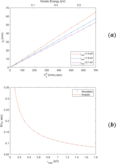 |
| | Fig. 4 (a) The final position on the detector as a function of the initial velocity, for electrons that are starting from the origin with initial velocity on y axis only, for different values of εmax. The continuous lines are given by the analytical derivation and the dots are given by the simulation. (b) The magnification as a function of εmax. | |
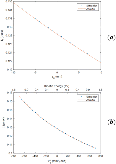 |
| | Fig. 5 (a) Time-of-flight for a beam of electrons starting from different positions along the ẑ axis between z0 = −10 mm to z0 = 10 mm, for x0 = y0 = 0, and for εmax = 1.8 eV. (b) Time-of-flight for a beam of electrons starting from the origin with velocity on z axis only for εmax = 1.8 eV. | |
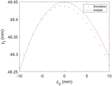 |
| | Fig. 6 Impact position yf as a function of the source position z0, for εmax = 1.8 eV. We used an electron beam starting from the origin with velocity on the y axis only, which corresponds to a kinetic energy of 1 eV. We observe very small deviations (less than 0.041%) that practically can be neglected, since they are smaller than the detector's resolution. | |
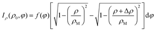
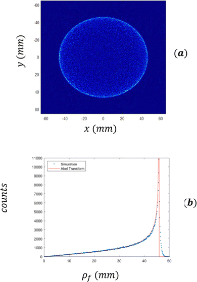
As a demonstration of the power of the device, Fig. 7(a), shows the simulated image produced on the detector for the case of 500![[thin space (1/6-em)]](https://www.rsc.org/images/entities/char_2009.gif) 000 electrons with an initial kinetic energy of εk = 0.9 eV, assuming that the direction distribution is spherically symmetric. The electrons were emitted from a cylindrical volume with a diameter of 80 mm (in the and ŷ directions) and were normally distributed along the ẑ direction with a standard deviation of 10 mm. Fig. 7(b) shows a histogram of ρf. The red line corresponds to the expected ρf distribution given by:
000 electrons with an initial kinetic energy of εk = 0.9 eV, assuming that the direction distribution is spherically symmetric. The electrons were emitted from a cylindrical volume with a diameter of 80 mm (in the and ŷ directions) and were normally distributed along the ẑ direction with a standard deviation of 10 mm. Fig. 7(b) shows a histogram of ρf. The red line corresponds to the expected ρf distribution given by:
| |  | (16) |
Here

, and Δ
ρ is the histogram's bin size. The match between this formula and the results of the simulations is good despite the formula neglecting broadening due to spherical aberrations.
 |
| | Fig. 7 (a) Expected image on the detector based on SIMION simulation with 500000 electrons with a kinetic energy of 0.9 eV, which start from a large initial volume (with a width of 80 mm). (b) The histogram of ρf. The red line corresponds to the expected Abel transform (eqn (3)). In both cases εmax = 1.8 eV. | |
4 Position imaging and mixed imaging
The quadratic potential presented above (eqn (2)) can also be used for position imaging (also known simply as ‘imaging’). In this case the goal is that ρf depends only on ρ0 and not on voρ. This can be achieved by setting the sine term in eqn (7) to zero, which is the case when ωρtf = πn for an integer n. Taking n = 1 leads to the condition:| |  | (17) |
with:| |  | (18) |
In this case the image is inverted without magnification. Fig. 8 shows an example of operating the CSR-ReMi in position imaging mode, where electrons produced from the same spot but with different velocities are imaged to the same spot.
 |
| | Fig. 8 SIMION demonstration of position imaging in the CSR-ReMi. Here values of Uρ = −6.7 × 10⁻³ V mm−2 and Uz = −0.2 V mm−2 are taken. The equipotential lines are shown in red. Also shown are two sets of trajectories. The blue trajectories correspond to electrons with kinetic energies in the 0–1 eV range which all start at y0 = −30 mm, and the green trajectories correspond to electrons in the same kinetic energy range starting at y0 = 10 mm. In both cases the different electrons are focused to a small spot on the detector at inverted positions (ρf = 30, −10 mm respectively). | |
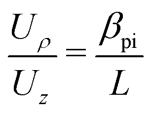
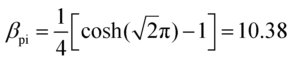
Another interesting possibility is a mixed imaging mode with position imaging along one axis and velocity map imaging in the perpendicular direction. In this case, the cylindrical symmetry is broken and therefore the implementation of this mode requires the construction of a dedicated spectrometer with elliptically shaped electrodes. Fig. 9 shows an illustration of a setup where such capabilities may be interesting, for studying thermionic emissions without the use of mass selection. In this case a hot ion beam, A−, is accelerated and directed through the electron spectrometer and then deflected into a Faraday cup. If a thermionic emission event occurs within the electron spectrometer, A− → A + e−, then the electron will be accelerated upwards (in the ẑ direction) and imaged on the E-MCP detector, while the neutral fragment will continue down stream (along the ŷ direction) and imaged, in coincidence, on a MCP for neutrals labeled ‘N-MCP’ in Fig. 9. Using the time delay between the impacts on the two detectors, one can determine the mass of the parent ion, if the distance to the detector is well known. By using position imaging in the ŷ direction one can deduce precisely the position of the ionization event and, thus deduce the mass with better resolution. Using VMI in the position allows determining the kinetic energy distribution of the electrons. Thus, one can measure the distribution of energies of thermionically emitted electrons for different ions simultaneously without the need for mass-selection. Mixed imaging can be achieved using the following solution of the Laplace equation:
| |  | (19) |
 |
| | Fig. 9 An illustration of a spectrometer for measuring the thermionic emission from anions without prior mass selection, as an example for an application of mixed imaging: velocity map imaging along the direction and position imaging in the ŷ direction which is used to determine the position of the ionization event. This information can be used to improve the time-of-flight determination of the parent ions mass. | |
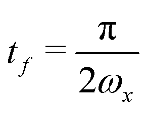
We define:  , and
, and  , and require, for mixed imaging that ωxtf = π/2, ωytf = π and ωy = 2ωx and therefore that:
In this case xf = −Mv0x where the magnification is  and yf = −y0. For z0 = v0z = 0 the solution for the equation of motion in the ẑ direction is given by:
| |  | (21) |
using

leads to an equation for
Uz:
| |  | (22) |
Thus, with given
εmax (the maximal kinetic energy to be measured),
Ux,
Uy and
Uz should be set according to:
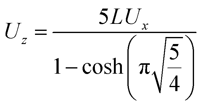
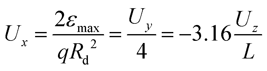
| |  | (23) |
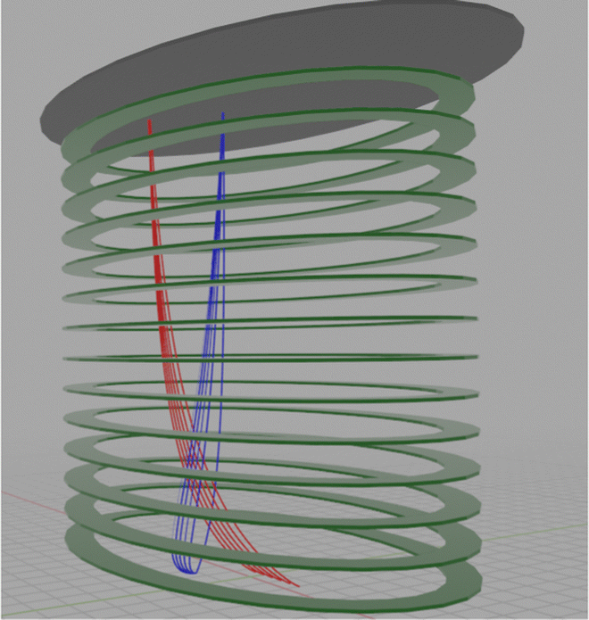
Fig. 10 shows an example of the results of a SIMION simulation of this kind of a device. Here a stack of elliptical electrodes with Rx = 40 mm and Ry = 20 mm is used. The red lines correspond to the trajectories of a series of electrons starting at different initial positions along the axis and focused to one point, while the blue trajectories are a series of electrons starting from the same point but having different v0y velocities, which are also focused to a single spot.
 |
| | Fig. 10 An illustration of mixed imaging. We chose here Ux = −3.75 × 10⁻³ V mm−2, Uy = −0.015 × 10⁻³ V mm−2 and Uz = −0.1782 × 10⁻³ V mm−2. The red trajectories correspond to electrons starting from the same y0 and having the same v0x (corresponding to a kinetic energy of 1 eV) but with a range of different x0. The blue trajectories describe electrons starting at y0 = 6 mm with different v0y which correspond to kinetic energies in the 0–1.25 eV range. Both sets of trajectories are focused to a small spot on the detector. | |
5 Conclusions
In conclusion, we have presented an analytical derivation showing how a quadratic potential can be used for velocity map or position imaging with no spherical aberrations. We have used SIMION simulations to demonstrate the applicability of these derivations to a practical device: as a means of operating the CSR-ReMi in a VMI mode so that it can be used for photo-electron spectroscopy. The simulations suggest 40-fold improvement of the focusing factor over the present state of the art. We have also shown how this methodology can be used in a mixed imaging mode and discussed one possible use for such a device.
Conflicts of interest
There are no conflicts to declare.
Acknowledgements
We are grateful to Oded Heber for insightful conversations and for suggesting to use the CSR-ReMi in VMI mode. This work was supported by the Israeli Science Foundation, the Minerva center for making bonds by fragmentation and by COST Action CA18212 (Molecular Dynamics in the GAS phase (MD-GAS)).
References
- M. L. Weichman and D. M. Neumark, Ann. Rev. Phys. Chem., 2018, 69, 4.1–4.24 CrossRef PubMed.
- R. Mabbs, E. Grumbling, K. Pichugin and A. Sanov, Chem. Soc. Rev., 2009, 38, 2169–2177 RSC.
- J. Cooper and R. N. Zare, J. Chem. Phys., 1968, 48, 942 CrossRef CAS.
- K. L. Reid, Ann. Rev. Phys. Chem., 2003, 54, 397–424 CrossRef CAS PubMed.
- A. Stolow, A. E. Bragg and D. M. Neumark, Chem. Rev., 2004, 104, 1719–1757 CrossRef CAS PubMed.
- A. I. Chichinin, K. H. Gericke, S. Kauczok and C. Maul, Int. Rev. Phys. Chem., 2009, 28, 607–680 Search PubMed.
- G. Basnayake, Y. Ranathunga, S. K. Lee and W. Li, J. Phys. B, 2022, 55, 607–680 CrossRef.
- A. G. Suits, Rev. Sci. Instrum., 2018, 89, 111101 CrossRef PubMed.
- A. T. Eppink and D. H. Parker, Rev. Sci. Instrum., 1997, 68, 6447 CrossRef.
- D. A. Horke, G. M. Roberts, J. Lecointre and J. R. Verlet, Rev. Sci. Instrum., 2012, 83, 063101 CrossRef PubMed.
- J. J. Lin, J. Zhou, W. Shiu and K. Liu, Rev. Sci. Instrum., 2003, 74, 2495–2500 CrossRef CAS.
- N. G. Kling, D. Paul, A. Gura, G. Laurent, S. De, H. Li, Z. Wang, B. Ahn, C. H. Kim, T. K. Kim, I. V. Litvinyuk, C. L. Cocke, I. Ben-Itzhak, D. Kim and M. F. Kling, J. Instrum., 2014, 9, P05005 CrossRef.
- B. Marchetti, T. N. Karsili, O. Kelly, P. Kapetanopoulos and M. N. Ashfold, J. Chem. Phys., 2015, 142, 224303 CrossRef PubMed.
- B. Ding, W. Xu, R. Wu, Y. Feng, L. Tian, X. Li, J. Huang, Z. Liu and X. Liu, Appl. Sci., 2021, 11, 10272 CrossRef CAS.
- R. Wu, B. Ding, Y. Feng, K. Wu, X. Jin and X. J. Liu, Meas. Sci. Technol., 2023, 34, 055502 CrossRef.
- M. Davino, E. McManus, N. G. Helming, C. Cheng, G. Mogol, Z. Rodnova, G. Harrison, K. Watson, T. Weinacht, G. N. Gibson, T. Saule and C. A. Trallero-Herrero, Rev. Sci. Instrum., 2023, 94, 013303 CrossRef CAS PubMed.
- R. V. Hahn, A. Becker, F. Berg, K. Blaum, C. Breitenfeldt, H. Fadil, F. Fellenberger, M. Froese, S. George, J. Göck, M. Grieser, F. Grussie, E. A. Guerin, O. Heber, P. Herwig, J. Karthein, C. Krantz, H. Kreckel, M. Lange, F. Laux, S. Lohmann, S. Menk, C. Meyer, P. M. Mishra, O. Novotný, A. P. O'Connor, D. A. Orlov, M. L. Rappaport, R. Repnow, S. Saurabh, S. Schippers, C. D. Schröter, D. Schwalm, L. Schweikhard, T. Sieber, A. Shornikov, K. Spruck, S. S. Kumar, J. Ullrich, X. Urbain, S. Vogel, P. Wilhelm, A. Wolf and D. Zajfman, Rev. Sci. Instrum., 2016, 87, 063115 CrossRef PubMed.
- R. Dörner, V. Mergel, O. Jagutzki, L. Spielberger, J. Ullrich, R. Moshammer and H. Schmidt-Böcking, Phys. Rep., 2000, 330, 95–192 CrossRef.
- J. Ullrich, R. Moshammer, A. Dorn, R. Dörner, L. P. H. Schmidt and H. Schmidt-Böcking, Rep. Prog. Phys., 2003, 66, 1463–1545 CrossRef CAS.
- H. Schmidt-Böcking, J. Ullrich, R. Dörner and C. L. Cocke, Ann. Phys., 2021, 533, 2100134 CrossRef.
- D. A. Dahl, Int. J. Mass Spectrom., 2000, 200, 3–25 CrossRef CAS.
|
| This journal is © the Owner Societies 2023 |
Click here to see how this site uses Cookies. View our privacy policy here. 
 *a
*a

 , and Uρ and Uz are constants.


 be the maximal electron kinetic energy to be measured (i.e., an electron with this energy with velocity on the


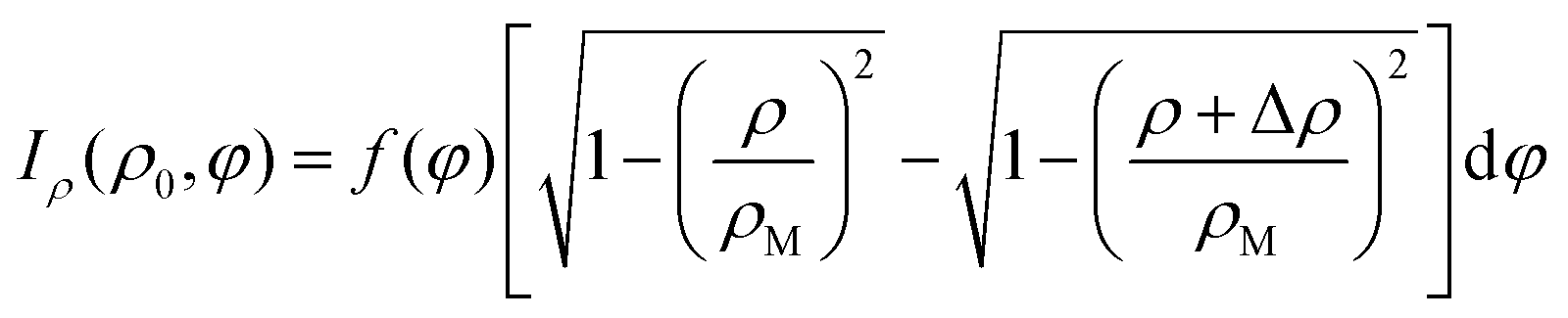
 , and Δρ is the histogram's bin size. The match between this formula and the results of the simulations is good despite the formula neglecting broadening due to spherical aberrations.


 , and
, and 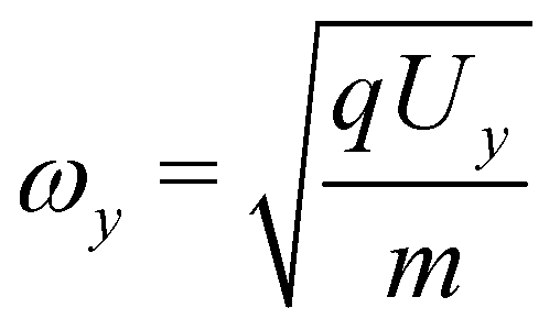 , and require, for mixed imaging that ωxtf = π/2, ωytf = π and ωy = 2ωx and therefore that:
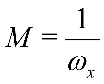 and yf = −y0. For z0 = v0z = 0 the solution for the equation of motion in the ẑ direction is given by:
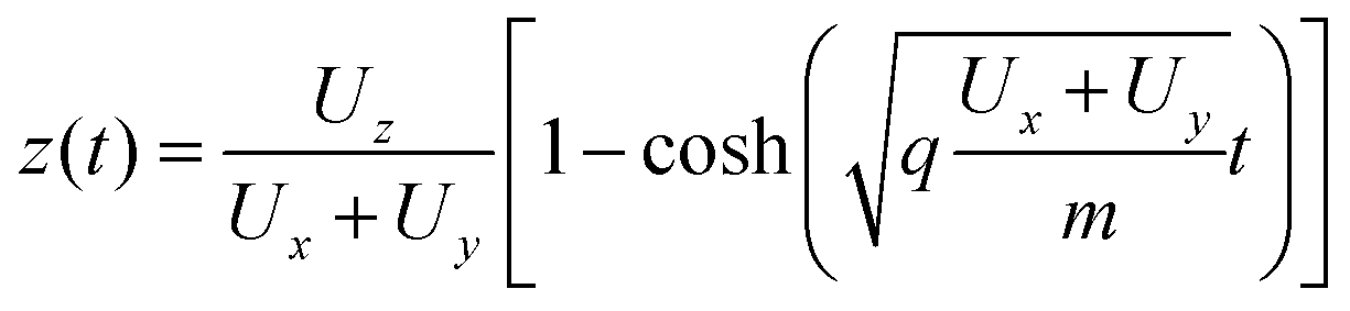
 leads to an equation for Uz: