DOI:
10.1039/D2NA00099G
(Review Article)
Nanoscale Adv., 2022,
4, 2583-2607
Solution NMR methods for structural and thermodynamic investigation of nanoparticle adsorption equilibria
Received
13th February 2022
, Accepted 7th May 2022
First published on 10th May 2022
Abstract
Characterization of dynamic processes occurring at the nanoparticle (NP) surface is crucial for developing new and more efficient NP catalysts and materials. Thus, a vast amount of research has been dedicated to developing techniques to characterize sorption equilibria. Over recent years, solution NMR spectroscopy has emerged as a preferred tool for investigating ligand–NP interactions. Indeed, due to its ability to probe exchange dynamics over a wide range of timescales with atomic resolution, solution NMR can provide structural, kinetic, and thermodynamic information on sorption equilibria involving multiple adsorbed species and intermediate states. In this contribution, we review solution NMR methods for characterizing ligand–NP interactions, and provide examples of practical applications using these methods as standalone techniques. In addition, we illustrate how the integrated analysis of several NMR datasets was employed to elucidate the role played by support–substrate interactions in mediating the phenol hydrogenation reaction catalyzed by ceria-supported Pd nanoparticles.
Introduction
Nanoparticle (NP) catalysts have found many applications in numerous fields such as energy,1,2 petrochemical,3,4 and medicine,5,6 due to their high surface-area-to-volume ratio and size-dependent properties that make them highly efficient and tunable catalysts. Since sorption equilibria play an essential role in determining the efficiency and selectivity of NP catalysis, many analytical techniques have been utilized to characterize ligand–NP surface interactions, including ultraviolet-visible (UV/Vis) spectroscopy,7–10 fluorescence,11,12 vibrational spectroscopy,11–13 and isothermal titration calorimetry (ITC).14 However, the outcomes of these analytical methods are generally dependent on the specific system under investigation and experimental conditions. In recent years, solution NMR spectroscopy has emerged as a preferred tool to investigate the interaction between the substrate and the NP surface. Indeed, due to its ability to probe dynamic processes occurring over a wide range of timescales (ps to hours), NMR spectroscopy is applicable to a broad range of NP–ligand pairs. In addition, the ability of NMR to provide data with atomic resolution allows a comprehensive characterization of the NP–substrate interaction, returning structural, kinetic, and thermodynamic information on the sorption equilibrium.
This contribution gives a brief overview of non-NMR techniques to investigate small molecule–NP interactions and the types of information these approaches can provide. In addition, we review solution NMR methods commonly employed in the characterization of small molecule–NP interactions, and we provide examples of their applications to various ligand–NP systems. Finally, we discuss how the combined analysis of multiple solution NMR methods was used to characterize the contribution of substrate–support interactions toward the hydrogenation of phenolic compounds catalyzed by ceria-supported palladium (Pd/CeO2) NPs.
Langmuir's theory
Experimental data on ligand–NP interactions are commonly analyzed within the framework of Langmuir's theory.15–17 The Langmuir model relies on four primary assumptions: (i) the adsorbent surface is homogeneous, (ii) each binding site can only hold one adsorbent molecule (i.e. monolayer coverage), (iii) adsorbed molecules do not interact with one another, and (iv) the adsorption process is reversible. Although modified models that address the limitations introduced by such assumptions were proposed,18–21 the original Langmuir isotherm model is, so far, the most common approach for modelling sorption equilibria.
The interaction between a ligand (L) and a vacant binding site on the surface (S) to form an adsorbed species (LS) can be represented in the form of a chemical equation:
| |  | (1) |
where
kads and
kdes are the rate constants for adsorption and desorption, respectively. However, while for a typical equilibrium process, the equilibrium constant (
Keq) is derived as the ratio between the concentrations of products and reactants (
i.e.
for
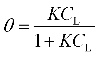
eqn (1)), for a surface sorption equilibrium in the Langmuir model, the concentration of binding sites is generally unknown and has to be part of the equation. The fraction of surface binding sites occupied by ligands is defined as the surface coverage (
θ):
| |  | (2) |
where
gLS is the grams of adsorbed ligand per gram of adsorbent and
gmax is the maximum adsorption capacity (in grams) that corresponds to the monolayer formation in the specific ligand–NP system under investigation. Therefore, the fraction of vacant sites will be expressed as 1 −
θ.
In the original gas-phase Langmuir model, rates of adsorption (rads) and desorption (rdes) are derived by means of the ligand pressure (p) and the surface coverage θ (rads = kadsp(1 − θ) and rdes = kdesθ, respectively). However, when applied to the liquid phase systems, the ligand amount is quantified in terms of molar concentration. Taking this and the fact that at equilibrium rads = rdes into account, the Langmuir isotherm model is generally represented in one of the two forms shown below:17
| |  | (3a) |
| |  | (3b) |
where
CL and
qLS are the concentrations of desorbed and adsorbed ligand at equilibrium, respectively,
qmax is the maximum adsorption capacity (in mol L
−1), and
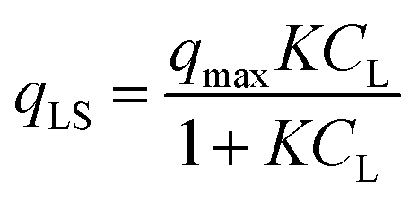
K is the Langmuir equilibrium constant that corresponds to the inverse of the equilibrium concentration of free ligand when half of the available adsorption sites are occupied (
Fig. 1). Therefore, like any equilibrium constant of an association process, the higher the value of
K, the stronger the ligand–NP interaction.
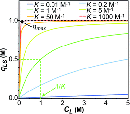 |
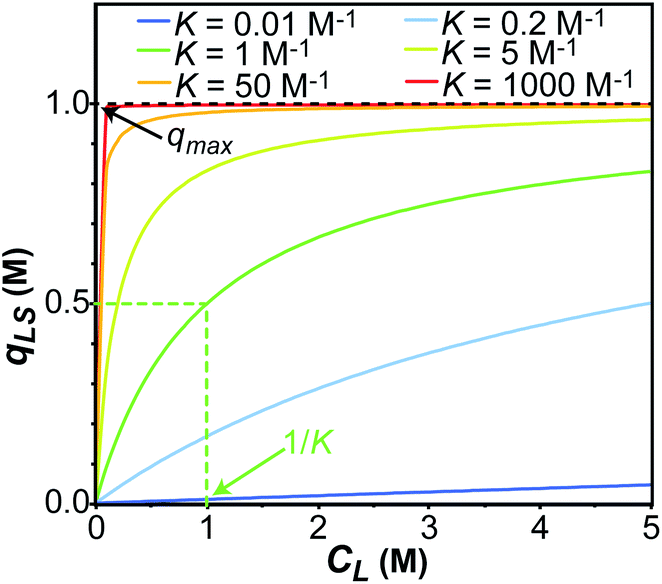
| | Fig. 1 Simulation of the concentration of surface adsorbed ligand (qLS) versus concentration of free ligand (CL) obtained using the Langmuir isotherm model (eqn (3)). Simulations were performed for Langmuir constants (K) of 0.01 (blue), 0.2 (light blue), 1 (green), 5 (yellow), 50 (orange), and 1000 (red) M−1. The maximum surface coverage (qmax) was set to 1 M (black dashed line). Half occupancy of the NP surface is obtained at CL = 1/K (shown with a green dashed line for the K = 1 M−1 simulation). | |
In an ideal adsorption study, qLS and CL are measured at increasing ligand concentrations, and the experimental isotherm resulting from plotting qLSversus CL is modelled using eqn (3b) to obtain qmax and K (Fig. 1). Although powerful in providing information on the number of adsorption sites (qmax) and strength of the NP–ligand interaction (K), the latter approach suffers from several experimental limitations. Indeed, accurate modelling of qmax and K can only be obtained if a range of ligand concentrations can be spanned so that qLS is measured at CL values that are much smaller and much larger than K−1. In the case where the range CL ≪ K−1 cannot be sampled (i.e. the analytical technique used to measure qLS and/or CL is not sensitive enough), the experimental isotherm will grow too steeply nearby CL ∼ K−1 to obtain an accurate estimate for the Langmuir constant (red and orange curves in Fig. 1). On the other hand, if conditions at which CL ≫ K−1 cannot be analyzed (i.e. the ligand and/or NP aggregate at a high concentration of small molecule), the experimental isotherm never reaches saturation (i.e. qLS ∼ qmax) and qmax cannot be accurately determined by modelling the experimental data (light blue and dark blue curves in Fig. 1). If the size and morphology of the investigated NP are known, the latter limitation can be circumvented by estimating qmax as the highest theoretical ligand density in a monolayer on the NP surface. Oftentimes, the value of K obtained by modelling adsorption data with eqn (3a) and (3b) is treated as a conventional equilibrium constant and used for the estimation of the free energy of adsorption (ΔGads) by means of the following relationship:
| | ΔGads = −RT![[thin space (1/6-em)]](https://www.rsc.org/images/entities/char_2009.gif) lnK lnK | (4) |
where
T is the temperature and
R is the universal gas constant. In such cases, care must be taken to the fact that the Langmuir equilibrium constant obtained by fitting experimental adsorption data is usually not dimensionless.
22 A recent publication reviews the topic in further details and summarizes mathematical approaches to transform the Langmuir constant into a dimensionless standard equilibrium constant compatible with
eqn (4).
23
In addition to providing estimates for thermodynamic parameters, the Langmuir model can be expanded for the investigation of adsorption kinetics. Generally, adsorption of ligands to NPs is described using either a pseudo-first-order (eqn (5))24 or a pseudo-second-order (eqn (6))25 kinetic model:
| |  | (6) |
In these models, A is an empirical constant that depends on the actual values of kads and kdes, kobs is the observed rate constant of the corresponding pseudo-first or pseudo-second kinetic process, and qt is the adsorbed amount of the ligand at each time point measurement. In many cases, experimental limitations require the introduction of a time delay factor (t0) that compensates for the time gap between the addition of ligands to the system and the collection of the data. As a result, the pseudo-first-order kinetic model is more often represented by the following equation:26,27
| | | θ(t − t0) = A(1 − e−kobs(t−t0)) | (7) |
Depending on the analytical method employed to investigate the adsorption kinetics, eqn (5)–(7) are often modified to accommodate substitution of θ with a directly measured observable.27
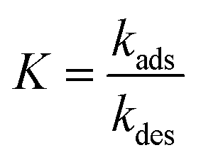
For processes that follow pseudo-first-order kinetics, an accurate determination of kads and kdes can be obtained if kobs is determined at several concentrations of ligands (L = CL + qLS). Since the rate constants are connected by the linear function kobs = kadsCL + kdes, the slope of the experimental kobs over CL plot provides the value of kads while the intercept with the y-axis yields kdes. Knowledge of the adsorption and desorption rate constants can be used to calculate the Langmuir equilibrium constant by means of the following equation:23
| |  | (8) |
Of note, the latter approach to the determination of K does not require estimation of qmax and is, therefore, the preferred method to obtain the Langmuir equilibrium constant for weak ligand–NP interactions.26 However, it should be noted that eqn (8) only applies to sorption equilibria based on elementary reactions. In the case of more complex equilibria involving one or more intermediate states, the ratio of the rate constants in eqn (8) would not provide an accurate estimate of K.23
Overview of analytical methods for characterizing sorption equilibria
Spectroscopic analytical techniques such as UV/Vis, IR, Raman, and fluorescence are the most developed methods for studying the binding of small molecules to NP surfaces, and a large number of studies are available in the literature that use these methods to obtain a qualitative description of binding as well as the necessary parameters for quantifying adsorption via the Langmuir theory. In addition, a variety of other analytical methods (i.e. X-ray,28,29 microscopy,30,31 SS-NMR,32–36etc.) have been sparsely applied to specific NP–ligand systems, but they have not found a general application for the characterization of sorption dynamics.
Ultraviolet-visible (UV/Vis) spectroscopy
UV/Vis is a sensitive and cost-effective spectroscopic method for the detection and characterization of diverse analytes, ranging from small molecules7–10 to large biopolymers.11,12 The UV/Vis adsorption wavelength of an analyte is highly sensitive to the immediate environment, and thus, different UV/Vis absorption maxima are expected for an adsorbed ligand and for the same molecule in the bulk solution. Due to this potential ability to differentiate among adsorbed and desorbed species, UV/Vis spectroscopy has been often used as a standalone technique for detecting ligand–NP adducts and, in some instances, to obtain structural and thermodynamic information on the interaction. However, the low resolution of UV/Vis spectra exposes a major drawback of this technique that often requires separation of the desorbed and adsorbed species via precipitation or filtration procedures for quantitative analysis. This sample preparation step hampers the characterization of weak ligand–NP interactions by UV/Vis spectroscopy.
Systems that involve the adsorption of proteins onto NPs are generally excessively complex for conventional UV/Vis and are normally characterized by Surface Plasmon Resonance (SPR).12 Formation of the NP–ligand conjugate results in a shifted and broadened adsorption spectrum. Since these changes are related to the concentration of bound species, SPR could yield quantitative binding parameters. Although this method is applicable to nearly any type of ligand, it is restricted to metal NPs capable of producing SPR spectra.
Quantitative analysis of binding.
The most common approach to quantitative analysis of small molecule–NP systems by UV/Vis involves exposing a standard ligand solution of known concentration (L) to a known amount of NPs and monitoring the changes in the concentration of free (CL) and surface adsorbed (qLS) ligand over time. Although CL and qLS could be in principle determined directly by observing the UV/Vis signals of the free and bound small molecule, respectively, the intrinsic low-resolution of UV/Vis spectroscopy hampers a direct quantification of the two species from a single spectrum. Therefore, CL is often determined from UV/Vis spectra measured on samples in which the adsorbed species is filtered or precipitated out of solution. The qLS value can be derived indirectly by subtracting CL from L, and the obtained data can be fit using the Langmuir adsorption model (eqn (5)–(8)) to yield the kinetics and thermodynamics of sorption. Employment of UV/Vis spectroscopy in this manner was reported for a few protein–NP and small molecule–NP systems, where the equilibrium association constant37–41 or a range of kinetic and thermodynamic parameters9,10,40–47 were determined.
In applications examining adsorption on noble metal NPs (generally gold), UV/Vis spectroscopy can be conveniently complemented by SPR.48 In this hybrid method, CL is obtained by UV/Vis as described above, while qLS is measured directly by observing the changes in the SPR spectrum of the NP caused by ligand binding.
The recent interest in DNA-based nanotechnologies ignited further development in the UV/Vis-based methods for quantifying NP adsorption. In particular, a novel quantitative colorimetric approach was introduced to assess the binding strength of DNA bases and nucleosides to silver39 and gold38 NPs. The approach relies on following colorimetric changes induced by aggregation of NPs upon ligand binding. As it was shown that the NP aggregation rate is directly correlated to the concentration of adsorbed ligand, CL and qLS can be obtained by the colorimetric assay.
Qualitative analysis of binding.
Interpretation of UV/Vis spectral changes can also provide valuable non-quantitative information about ligand binding. Indeed, a change in peak position in the spectrum of a ligand upon the addition of NP can indicate the occurrence of ligand–NP interaction. In addition, analysis of these spectral changes in comparison to known references could return structural insight into the mode of interaction. For example, de Haan et al. found that the changes in the UV/Vis spectrum of alizarin in the presence of ZnO NPs are consistent with the absorbance spectrum observed for deprotonated alizarin, suggesting that alizarin binds to ZnO NPs in its deprotonated form.8
Fluorescence
Fluorescence spectroscopy and its variations, such as Fluorescence Correlation Spectroscopy (FCS), are convenient techniques for investigating adsorption processes due to their high intrinsic sensitivity and their ability to provide input experimental data for the Langmuir isotherm model. The fluorescence of ligands is highly sensitive to quenching by the formation of NP–ligand conjugates. Therefore, analysis of the changes in fluorescence spectra (i.e. intensity, broadening, a shift in emission maxima) provides qualitative, and in some cases quantitative, insight into sorption processes.
Although fluorescence was used to study the adsorption of proteins and small fluorescent molecules (dyes) onto NPs,11,12 the need for the ligand or the NP to be either naturally fluorescent or to carry a covalently attached fluorescent label has limited its broader applicability to the study of sorption equilibria. In addition, if NPs are not removed from the solution (by filtration or centrifugation) before the fluorescence measurement is taken, they have the potential to induce inner filter and light scattering effects that complicate the analysis of the data.49,50
Quantitative analysis of binding.
Three main fluorescence-based approaches to derive quantitative information for NP–ligand systems were described for inherently fluorescent small molecules and proteins. The Fluorescence Quenching Titration (FQT) method exploits the ability of NPs to quench the fluoresce of bound ligands. Therefore, the solution of a fluorescent ligand is titrated with NP to achieve complete quenching of the signal. Plotting the normalized fluorescence intensity over concentration of NP yields a nonlinear decay that is modelled to provide the estimated binding constant.51 This methodology found wide application in examining both protein–NP12 and small molecule–NP52 interactions. In addition to estimation of binding constants, the fluorescence quenching method could serve as a tool for examining the accessible surface area. For example, the Molecular Probe Adsorption (MPA) method demonstrated the convenience of fluorescence spectroscopy for estimating the available adsorption surface in NPs containing a corona phase.53
The Fluorescence Correlation Spectroscopy (FCS) method provides several advantages over FQT. FCS relies on measuring variations of fluorescence produced by species that diffuse through a part of a sample that is actively monitored by a laser beam. This technique is highly sensitive and can detect exceptionally low concentrations of fluorophores, as low as nM. In addition, it does not suffer from complications that arise when measurements are performed with NPs present in the solution. Since the fluorescence of the free ligands can be measured independently from the molecules bound to NPs, the primary outcome of FCS is CL, while qLS is derived mathematically based on the measured concentration of the desorbed ligand. A well-illustrated example that studied the adsorption of fluorescent compounds rhodamine 6G and calcein on colloidal silica and alumina NPs showed the applicability of FCS to small molecule–NP systems.54
Finally, if the ligand and the NP of interest are not intrinsically fluorescent, a competition assay can be applied to characterize NP adsorption. This method is based on exposing the NP loaded with a surface-adsorbed fluorescent molecule to a solution of the non-fluorescent ligand. The release of the fluorescent probe from the NP surface is then monitored to determine the concentration of the non-fluorescent ligand that is adsorbed on the NP surface. The approach was demonstrated using fluorescently labeled oligonucleotides bound to gold NPs through an alkanethiol linker and mercaptoethanol as a displacing agent.55
Qualitative analysis of binding.
Qualitative analysis of fluorescence spectra was utilized to examine surface characteristics of ligand–NP systems such as charge density,56 functional group density, dielectric constants,57 and interfacial pH.58 Despite the very high sensitivity of fluorescence-based techniques and their ability to provide in situ measurements allowing for characterization of dynamic adsorption processes, the inherent challenges (among them the requirement for the fluorescently active ligands and a complicated experimental setup) dramatically limited the extent of studies of small molecules–NP binding thus far.
Vibrational spectroscopy
Interpretation of changes in the vibrational spectra of molecules upon adsorption on a surface was shown to be a highly versatile and convenient approach to yield experimental data necessary for qualitative and quantitative analysis of surface sorption. The two primary vibrational spectroscopy techniques are Fourier-Transform Infrared (FTIR) and Raman spectroscopies. The relative simplicity of sample preparation and data collection resulted in an extensive utilization of these methods for investigating sorption equilibria.
Fourier-transform infrared (FTIR) spectroscopy
The use of FTIR to characterize ligand–NP interactions relies on the ability of IR spectroscopy to detect the establishment of new functionalities in the sample (i.e. a ligand–NP bond) or the spectral perturbation of an IR-active functional group within the ligand or NP upon binding.11–13 Although the high complexity of FTIR spectra has limited their application to the characterization of small molecule–NP interactions,59–66 the more recent introduction of Attenuated Total Reflectance Fourier Transform Infrared (ATR-FTIR)13,67–75 and Surface-Enhanced Infrared Absorption (SEIRA)13,76–79 has expanded the use of IR-based methods to ligand–NP systems of higher complexity.
Quantitative analysis of binding.
Qualitative assessment of capping layers and functionalization at the NP surface is the primary outcome of IR-based techniques. Nonetheless, a carefully designed experiment that includes the necessary standard calibrations could provide a quantitative description of surface coverage as well as the thermodynamic and kinetic parameters of sorption.67 In the most common quantitative application, the time-dependent intensity change in the ATR-FTIR peaks corresponding to the adsorbed ligand is used to asses time-dependent changes in concentrations of the bound species and obtain the adsorption and desorption rate constants. This approach works best for slow adsorption processes that reach equilibrium at a slow enough rate to allow for data collection at multiple time points (typically minutes to hours), and was successfully applied to investigate the binding of small molecules on TiO2,80–87 iron (oxyhydr)oxides,88 hematite,89,90 Pt/Al2O3,91 and CeO2 NPs.92 In some of these studies, the adsorption and kinetic data were used to derive the Langmuir equilibrium constant using eqn (8).83–85,92
Qualitative analysis of binding.
Two-dimensional infrared spectroscopy (2D-IR)93,94 provides a high-resolution picture of the IR-active functionality in the investigated sample and has been utilized in several qualitative investigations of surface adsorption. For example, 2D-IR spectroscopy allowed the characterization of the structure and mobility of the capping layer comprised of amide and carboxylate-containing ligands on gold NPs.95 In another application, Bian et al. demonstrated the ability of multiple-mode multi-dimensional IR to obtain a complete picture of the conformations sampled by 4-mercaptophenol bound to gold NPs.96 2D-IR was also employed to study the conformations sampled by the tripeptide glutathione (used a capping layer) on the surface of silver NPs97,98 and their dependency on the NP size.97 In another example, 2D-IR was used to detect the Pt–H bond formed upon H2 activation on Pt99 and the aggregation of a complex organometallic dye on the surface of TiO2 NPs.100
Raman spectroscopy
One of the main advantages of Raman over IR spectroscopy for the analysis of sorption equilibria is its ability to perform measurements in aqueous environments since water does not interfere with Raman spectra. However, its lower sensitivity has hampered a broader application of the technique. The more recently introduced Surface-Enhanced Raman Scattering (SERS)101–103 overcomes the low sensitivity limitation of conventional Raman spectroscopy and, under certain circumstances, could even provide single-molecule resolution.104–108 The number of reported studies that employ SERS to examine surface processes has been rising in the last few years, and we expect the utilization of this technique to study NP adsorption will be much broader in the near future.
Quantitative analysis of binding.
There is no standard methodology for the utilization of Raman-based techniques to quantify sorption processes on NPs. However, several recent illustrations include carefully designed experimental protocols capable of providing quantitative data for the chemisorption of small molecules. Similar to the ATR-FTIR technique mentioned above, change in intensity for well-observed SERS bands of ligands interacting with NP can be plotted as a function of time and fit to a Langmuir adsorption model to result kobs for the interaction, as was illustrated by adsorption of 4-aminothiophenol and 2-thio-5-nitrobenzoic acid on gold NPs.27 One of the most comprehensive examples of SERS application to the ligand–NP system was illustrated by a very detailed investigation of the influence of surface curvature of nanotextured gold NPs on the binding of thiolated ligands.109 In this study, a wide range of structural, kinetic, and thermodynamic data were obtained using plasmon-enhanced Raman scattering. A robust methodology for determining ligand packing density and concentrations of bound and free substrates by SERS relies on utilizing isotopically labeled versions of the ligands as internal standards. Under this protocol, SERS can deliver the equilibrium constant by fitting the experimental data with the Langmuir adsorption model.110,111 However, the requirement for the labeled substrates has significantly limited the broader application of this method. A newly introduced approach called “Hot Spot”-Normalized Surface-Enhanced Raman Scattering (HSNSERS) not only eliminates the need for additional internal standards by utilizing surface-enhanced elastic scattering for calibration purposes but also allows for real-time observation of ligand exchange process in situ.112 Application of the HSNSERS technique was initially demonstrated by examining the interaction between several chloroanilines and gold NPs.112 A few additional studies expanded the utilization of this methodology.113,114
Qualitative analysis of binding.
SERS has found widespread application in qualitative analysis of ligand–NP interactions, providing important information on the binding mode of ligands on the NP surface.45,46,48,111,115–137 However, this technique nearly always has to be accompanied by other supporting methods, either theoretical (i.e. DFT, surface selection rules)127–131 or experimental (i.e. XPS, FTIR, UV/Vis),118,127 to aid in the interpretation of the results.
Isothermal titration calorimetry (ITC)
Isothermal Titration Calorimetry (ITC) is a versatile technique for examining thermodynamic and, in some cases, kinetic parameters on molecular interactions.138–140 The ability of ITC to directly measure ΔH of binding makes it stand out from the rest of the available methods. ITC data collection is performed by measuring the heat adsorbed or released when small aliquots of ligand solution are injected into a sample containing the NP receptor, and binding takes place. Fitting the titration curve (heat over ligand/receptor molar ratio) delivers a complete set of thermodynamic (ΔH, ΔS, and ΔG) and stoichiometric parameters of binding.
Quantitative analysis of binding.
ITC has been extensively utilized to study biomacromolecular interactions141 and, more recently, extended to the examination of other types of ligand-receptor systems. In particular, ITC was used to quantify the affinity of ligands towards the NP surface and guide the rational design of NP receptors with regulated binding strength towards specific targets.142,143 In the drug-delivery field, ITC derived data are used to quantify the loading of active pharmaceutical ingredients on NP delivery vehicles.144 In addition, ITC was reportedly used to characterize the thermodynamics of a few other ligand–NP systems.52,145,146
Qualitative analysis of binding.
Although quantitative analysis of binding is seen as the main strength of the ITC technique, a quick qualitative assessment of relative affinity trends could be performed on a series of compounds without the need for theoretical modelling of the experimental data. For example, using ITC data recorded for several DNA bases and their peptide analogs in the presence of gold NPs, Gourishankar et al. determined relative binding affinities of the ligands toward gold NPs.147
Despite the ability of ITC to yield near-complete thermodynamic characterization of binding, its broader application to the small molecule–NP system has been hampered due to experimental challenges and complexities involved in data processing. Among these, relatively long experimental times, interference from the aggregation of the investigated substrates and NPs, significant complications in assessing very weak and very strong bindings (K < 103 M−1 and K > 108 M−1, respectively), and the requirement to account for every contribution to heat in the studied system are generally considered the principal challenges of the ITC technique.
Solution NMR methods for characterizing sorption equilibria
NMR signals originate from low-energy transitions that relax slowly compared to other spectroscopic methods (ms–s). Although this property dooms NMR to the rank of a poorly-sensitive technique, it also provides NMR with several advantages over other analytical methods. Indeed, the low relaxation rate of its signals makes NMR a high-resolution method capable of returning different spectroscopic peaks for the different atoms composing the analyte under investigation. In addition, the fact that NMR excited states are long-lived allows extensive spectroscopic manipulations of the NMR signals that resulted in the creation of an unmatched portfolio of NMR experiments able to characterize dynamic processes occurring on timescales ranging from picoseconds to hours. This ability to probe with atomic-resolution dynamic interactions occurring on a large range of timescales makes NMR an ideal method for studying sorption equilibria that involve multiple adsorbed and intermediate states.
In this section, we review solution NMR methods for the investigation of surface adsorption. Before diving into specific NMR experiments, we will introduce the concept of chemical exchange as applied to solution NMR. Due to their large molecular size, NPs exhibit a large transverse relaxation rate (R2). Because of the large R2, NMR signals of NPs are broadened out beyond the detection level of conventional solution NMR spectroscopy (discussed in detail below). For this reason, the study of surface adsorption by direct investigation of NPs themselves using solution NMR techniques is often impossible, and solid-state NMR techniques are more often applied to this end.32,148,149 However, in the presence of a chemical exchange equilibrium between a free NMR-visible state and a NP-bound NMR-invisible state, several solution NMR experiments (reviewed below) can be used to imprint information on the structure and dynamics of NP surface-bound species into the spectrum of the free ligand. Therefore, the concept of chemical exchange is crucial for solution NMR studies of surface adsorption.
Chemical exchange in NMR
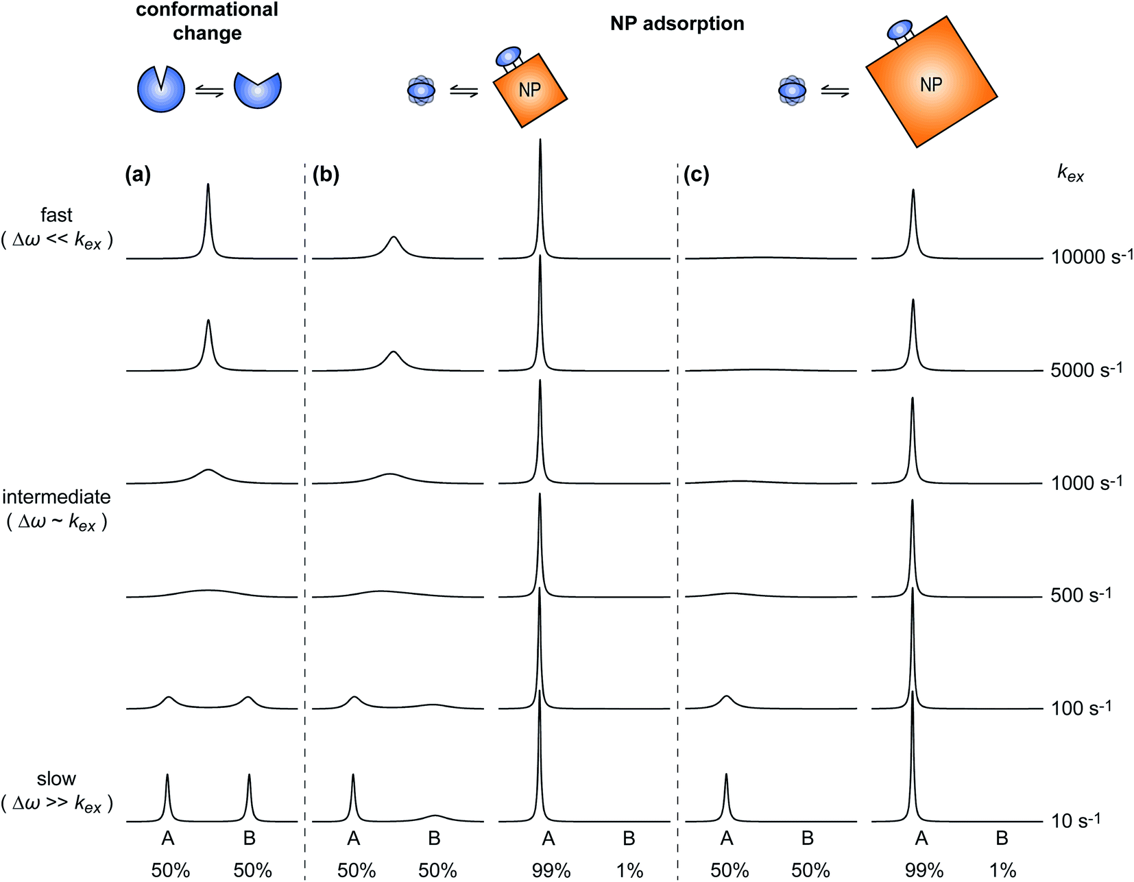
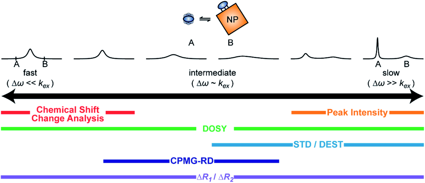
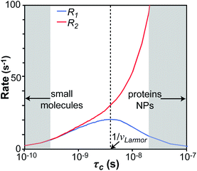
A process that involves a nucleus exchanging between different chemical environments is called a chemical exchange. In the context of this review, the binding of a small molecule to a NP surface is an example of chemical exchange. The chemical exchange induces changes in the NMR spectrum, and the appearance of the spectrum depends on the timescale in which the exchange occurs.150–153 There are three main timescales associated with NMR when describing chemical exchange: slow, intermediate, and fast. Each exchange regime can be defined in terms of a chemical shift difference (Δω), relaxation rates of the exchanging species, and exchange rate constant (kex). In this review, we will use a two-state exchange model to illustrate how exchange affects the NMR spectrum and will refer to this model to simulate data (Fig. 2).
 |
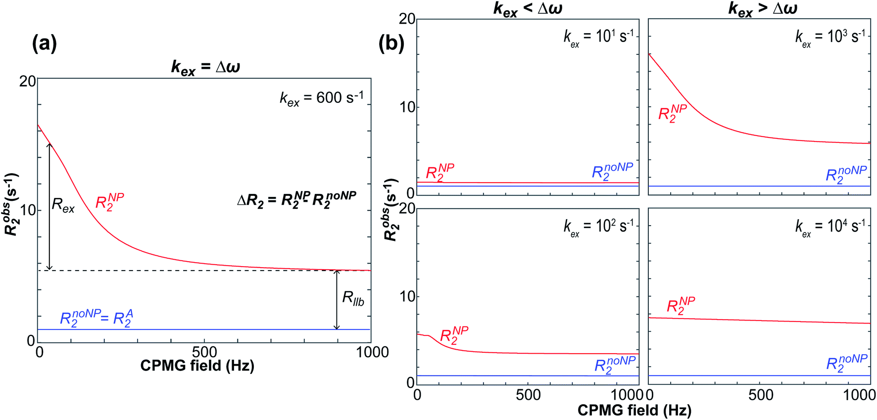
| | Fig. 2 Simulated NMR spectra illustrating the effect on the NMR lineshape of chemical exchange between two states, A and B, over a range of exchange timescales (0 to 10000 s−1, bottom to top). In (a), states A and B have an equal population (pA = pB = 0.5) and transverse relaxation rates (RA2 = RB2 = 10 s−1). In (b), RA2 = 10 s−1 and RB2 = 100 s−1 to simulate a sorption equilibrium in which a small molecule adsorbs on a small NP. In the left panel, the populations of desorbed (state A) and adsorbed (state B) species are considered equal (pA = pB = 0.5). In the right panel, the equilibrium is skewed toward state A (pA = 0.99 and pB = 0.01). In (c), RA2 = 10 s−1 and RB2 = 1000 s−1 to simulate a sorption equilibrium in which a small molecule adsorbs on a large NP. In the left panel, the populations of desorbed (state A) and adsorbed (state B) species are considered equal (pA = pB = 0.5). In the right panel, the equilibrium is skewed toward state A (pA = 0.99 and pB = 0.01). In all simulations, the chemical shift difference between states A and B (Δω) is 600 rad s−1. Note that the larger is RB2 and the more apparent is the effect of the small molecule–NP interaction on the NMR spectra of the ligand. Therefore, the larger is the NP size and the higher is the sensitivity of solution NMR in detecting and characterizing sorption. | |
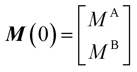
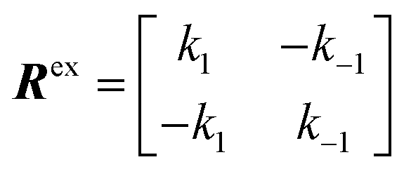
Consider a two-state model where a molecule is in an exchange between state A and state B:
| |  | (9) |
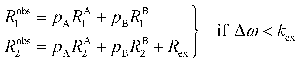
The two states are assumed to have different chemical shifts (i.e., Δω ≠ 0). k1 and k−1 are the forward and reverse first-order rate constants for the equilibrium (corresponding to kads and kdes in eqn (1), respectively), and kex = k1 + k−1.150–153 For simplicity, we will first consider a two-state model where the two exchanging species have similar longitudinal (R1) and transverse (R2) relaxation rates (RA1 ∼ RB1 and RA2 ∼ RB2, respectively) such as in equilibria describing a conformational change. It is important to note that this is not the case for the small molecule–NP system, which will be discussed later. Fig. 2a illustrates the effect of the exchange on the NMR spectrum of a molecule containing a single NMR-active nucleus. In the fast exchange regime (Δω ≪ kex), a single peak at the population-averaged chemical shift is observed. The observed relaxation rates will also be population-weighted:
| | | Robs1 = pARA1 + pBRB1 | (10) |
| | | Robs2 = pARA2 + pBRB2 | (11) |
where
Robs1 and
Robs2 are the observed longitudinal and transverse relaxation rates, respectively (note that one single peak is detected in the fast exchange regime), and
pA and
pB are the fractional populations of states A and B, respectively. On the contrary, in the slow exchange regime (Δ
ω ≫
kex), two peaks are observed, one at the chemical shift of state A and the other at the chemical shift of state B, each relaxing at its own relaxation rates. When the conditions for fast or slow exchange do not apply (
i.e. Δ
ω ∼
kex), the system is considered to be in the intermediate exchange regime, and the
Robs2 is enhanced by the exchange contribution,
Rex:
| | 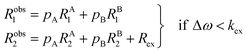 | (12) |
| |  | (13) |
where
Robs,A1 and
Robs,A2 are the
Robs1 and
Robs2, respectively, for the NMR peak of species A in the slow-intermediate exchange regime.
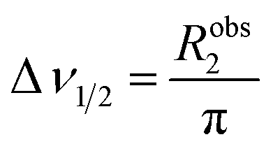
The appearance of the NMR spectrum is chiefly dependent on Robs2, as the linewidth (peak width at half height measured in Hz) of each NMR signal (Δν1/2) is given by:
| |  | (14) |
Therefore, the increase in Robs2 caused by Rex results in broadening of the detected signal and consequential reduction in intensity (note that the integral of the NMR signal is not affected by the exchange and, therefore, a larger linewidth is associated with a lower peak height). As shown in Fig. 2a, starting from the slow exchange regime and increasing kex, the two peaks will gradually broaden as a result of the exchange. When Δω ∼ kex the peaks will coalesce into one single NMR signal that is highly broadened by the chemical exchange. Further increase in kex will shift the system to the fast exchange regime with a consequent increase in resolution and peak intensity.
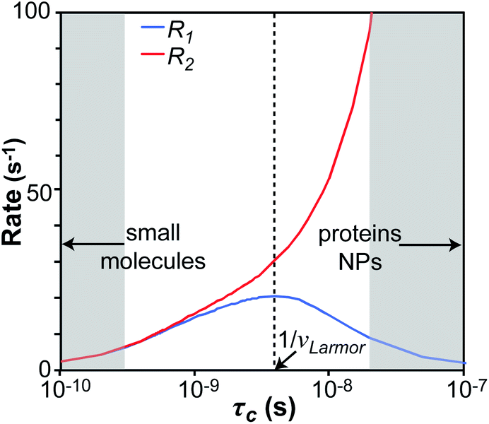
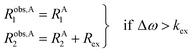
We will now consider a two-state model where a molecule is in equilibrium between the free and NP-bound states. Since the two states under chemical exchange differ considerably in molecular size, the dependency of the NMR relaxation rates from the molecular rotational tumbling needs to be taken into account when discussing the effect of the exchange on the measured NMR spectra. As shown in Fig. 3, the R1 reaches a maximum when the rate of rotational tumbling (1/τC, where τC is the rotational correlation time) is on the same order as the Larmor frequency of the observed nucleus. Although this condition depends on the nucleus under investigation (i.e.1H and 13C have different Larmor frequencies) and on the static field of the spectrometer, the fact that R1 is small for very small and very large molecules makes RA1 ∼ RB1 in the majority of the small molecule–NP systems (Fig. 3). On the other hand, the R2 always increases by increasing τC (Fig. 3), and RA2 ≪ RB2 for small molecule–NP sorption equilibria. The large RB2 often results in line broadening beyond detection level and, as a result, the NP-bound state becomes invisible by NMR (see Fig. 2b and c). However, despite its invisibility, the surface-bound state can affect the relaxation rate and chemical shift of the NMR-visible free molecule via chemical exchange (Fig. 2b and c), and a number of NMR experiments were developed to use the perturbation of the NMR signals of the NMR-visible state to obtain information on the NP-bound species.
 |
| | Fig. 3 Simulation of 13C relaxation rates as a function of correlation time at 800 MHz. Simulations were performed for a C–H spin system of fixed bond length (1.09 Å) using eqn (51) and (52). The longitudinal relaxation rate (R1) increases as τC increases, reaches a maximum when the rate of rotational tumbling matches that of Larmor frequency (i.e. when τC = 1/νLarmor), and decreases as the tumbling rate becomes slower than Larmor frequency (blue curve). The transverse relaxation rate (R2) increases as τC increases (red curve). Transparent gray boxes highlight the ranges of τC expected for small molecules (left) or proteins and NPs (right). | |
Fig. 2b and c show how the chemical exchange between two states with a large difference in R2 affects the NMR spectra at different timescales. In the fast exchange regime, a single peak is observed with population-weighted chemical shift and relaxation rates (eqn (10) and (11)). However, since the transverse relaxation data measured in the presence of NP are often analyzed in comparison to the R2 of the free state, the following equation is more commonly used:
where the lifetime line broadening (
Rllb) describes the increase in the observed transverse relaxation of state A caused by the exchange with a state with a higher
R2. In the intermediate exchange regime,
eqn (12) and
(13) still apply for
R1. On the other hand, the
R2 of the NMR-visible peak is given by:
| | | Robs,A2 = RA2 + Rex + Rllb | (16) |
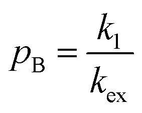
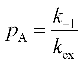
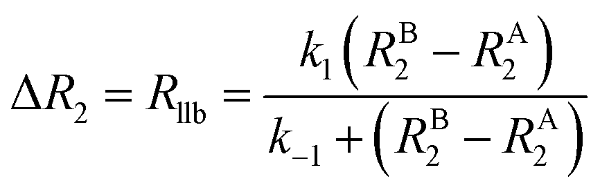
It is important to note that while Rllb is caused by the exchange between states with a large difference in R2, Rex is due to the exchange between states with different chemical shifts. Therefore, Rllb occurs even for exchange processes with Δω = 0. In the slow exchange regime, when the transverse relaxation rate of the NMR-invisible state is faster than dissociation from the bound to the free state (i.e. RB2 > k−1), the observed R2 is increased by the apparent rate of the forward reaction (i.e. Rllb = k1):154
This is because any binding event results in an irreversible loss of magnetization as the signal is completely relaxed before the small molecule returns to the NMR-visible free state. When this limiting condition does not apply, Rllb < k1 (see below).
In summary, the theoretical considerations discussed in this section indicate that although NP-bound species are not observed directly by solution NMR, the contrast between the fast R2 of the bound state and the slow R2 of the free state can be utilized to imprint information about the NP-bound state onto the spectrum of the NMR-visible free state. Given that the R2 of the visible state is affected differently depending on the timescale of the free-bound equilibrium, the types of solution NMR methods one can use to characterize NP adsorption are also dependent on the timescale in which the exchange occurs. In the following sections, we discuss solution NMR methods for characterizing small molecule–NP interactions at different exchange regimes.
Preparation of stable NMR samples containing nanoparticles
Solution NMR methods to investigate sorption equilibria rely on the direct observation of the ligand–NP adduct (in the case the investigated complex is small enough to be directly detected in a NMR experiment) or on the indirect observation of the NMR-invisible ligand–NP interaction on the spectra of the NMR-visible free ligand (see above). In either case, to obtain accurate and reproducible data, it is important that the ligand and the NP remain homogeneously suspended within the sample throughout the experiment. For soluble NPs, no special procedure is required to prepare NMR samples since the ligand-to-surface ratio will stay consistent throughout the sample and will not change over time. On the contrary, insoluble NPs quickly sediment in solution, changing the concentration of ligand–NP adduct within the NMR active volume over time. Therefore, establishing a generally applicable sample preparation method that results in homogeneously dispersed stable suspensions of insoluble NPs was a crucial step toward increasing the applicability of solution NMR methods to the characterization of sorption equilibria. The method consists in preparing the NMR samples in a gel matrix that prevents NP sedimentation.155,156 Such gel matrix should (i) undergo rapid gelation (which allows stabilization of a homogeneous suspension of NPs), (ii) not interfere with the ligand–NP interaction of interest, and (iii) have a minimal fingerprint in the NMR spectrum used for characterizing the ligand–NP system. A library of small molecule gelators that satisfy these requirements was recently developed to stabilize NP suspensions in a number of NMR-friendly aqueous155 and organic solvents.156
When discussing sample preparation protocols, it is also important to mention that indirect detection of the NMR-invisible ligand–NP adduct on the spectra of the NMR-visible free ligand is usually performed on samples in which the sorption equilibrium is highly skewed toward the free state (pA ≥ 90%). Indeed, the large R2 of the NP-bound state results in line broadening of the NMR signals of the free state even when pB ≤ 1% (note that the exact detection limit depends on RB2, with higher RB2's resulting in higher sensitivity), and a pB > 10% often results in a complete loss of signal (Fig. 2b and c).
Analysis of chemical shift changes (CSCs)
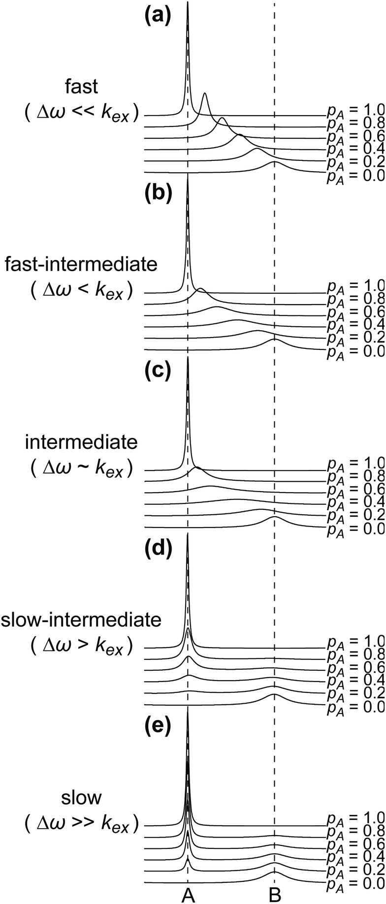
The NMR chemical shift is very sensitive to the local chemical environment of the nucleus. Therefore, chemical shifts are very sensitive reporters of intermolecular interactions. In a conventional CSC experiment, the NMR-visible interaction partner (i.e. the ligand) is kept at a constant concentration, while the NMR-invisible component of the interaction (i.e. the NP) is titrated into the solution, and the chemical shift change is monitored as a function of the titrant concentration. Fig. 4 illustrates how the NMR spectrum of a small molecule ligand changes upon the titration experiment within the fast, intermediate, and slow exchange regimes. To construct the spectra in Fig. 4, a simple two-state binding model was assumed. Analysis of this figure reveals that no chemical shift change is detected for processes occurring on the slow exchange regime since separate peaks are observed for the free and bound states with changes in peak intensities (discussed below) as the NP is titrated into the ligand (Fig. 4e). At the slow-intermediate exchange regime, a low population of the bound state (≤20%) results in a small CSC, while a high population of the bound state (≥50%) causes extreme line broadening due to Rex. These effects make monitoring the changes in chemical shift challenging for systems with binding kinetics in the slow-intermediate regime (Fig. 4b–d). Analysis of chemical shift change works best for weak binding interactions that occur on a fast timescale. In the latter case, the observed chemical shift (δobs) is a weighted average of the free and bound states chemical shifts (δA and δB, respectively):
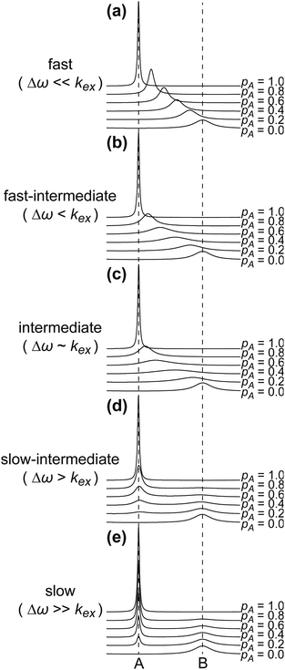 |
| | Fig. 4 Simulated NMR spectra showing the effect of varying the population of state A (pA) in a two-state sorption equilibrium occurring on the (a) fast exchange regime (kex = 104 s−1), (b) fast-intermediate exchange regime (kex = 103 s−1), (c) intermediate exchange regime (kex = 600 s−1), (d) slow-intermediate exchange regime (kex = 102 s−1), and (e) slow exchange regime (kex = 10 s−1). In all simulations, RA2 = 10 s−1, RB2 = 100 s−1, and Δω = 600 rad s−1. The vertical dashed lines indicate the chemical shifts of states A and B. | |
The CSC is measured in reference to the chemical shift of the free state, as described by the following equation:
| | | CSC = δobs − δA = (δApA + δBpB) − δA | (19) |
Given that pA + pB = 1, a rearrangement of eqn (19) gives:
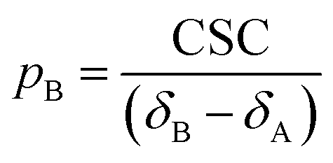
| |  | (20) |
Although the ability of the CSC analysis to return the concentration of bound ligand makes these experiments a potential input for the Langmuir isotherm modelling (e.g., pB ∼ θ in eqn (3a)), CSC experiments are associated with several practical problems that hamper their widespread use in quantitative studies of sorption. Indeed, as pB approaches 1, the NMR signal may become invisible due to the large R2 of the bound state. Moreover, since most NPs are sparingly soluble, obtaining near saturation of binding (required for accurate modelling of the Langmuir isotherm – see above) can be challenging, especially for the weak ligand–NP interactions that can be analyzed quantitatively by CSC. As an alternative, one can titrate the ligand into a fixed concentration of NP. In this case, the population of the bound state will decrease as the ligand is titrated in, eventually reaching close to 0 for concentrations of ligand much higher than K. However, it should be noted that the latter approach still suffers from the low sensitivity at low ligand concentrations (when most of the ligand is in the NMR-invisible bound state) and cannot be applied to ligands that oligomerize or precipitate at a concentration higher than K.
Despite all the challenges of CSC, analysis of the NP-induced changes in chemical shifts can still be used to characterize the functionalities involved in the interaction and the binding mode. For example, Calzolai et al. determined the location of the interaction site between the ubiquitin and gold NP by analyzing CSCs.157 They observed that the chemical shifts of only specific residues of ubiquitin changed upon the addition of gold NPs, revealing that the interaction is specific. Similarly, the binding sites for C60 fullerene in proteins were identified using CSC analysis.158,159 Also, by monitoring the interaction between L-lysine and water-soluble ruthenium NPs by CSC analysis, Martinez-Prieto et al. revealed that the binding orientation of L-lysine on the NP surface is relevant to the deuteration reaction catalyzed by the NP.160
In some cases, the study of surface adsorption on a metal surface using CSC can be hindered by the extreme broadening and peak shift caused by the Knight-shift effect.161,162 One way to overcome this disadvantage is to have a spacer atom between the observed nucleus of the adsorbed species and the metal surface. For example, using oxygen as the spacer atom, Tedsree et al. investigated the chemisorption of formic acid on various metal colloid catalysts and found that the 13C chemical shift values of the adsorbates were directly correlated to the chemisorption strength.163
Peak intensity
The NMR signal intensity (intended as the integral of the NMR peak) is related to the number of nuclei resonating at a given chemical shift. Therefore, the intensity of an NMR signal can be used to determine the concentration of a species in the analyzed sample. If a ligand undergoes chemical exchange between the free and NP-bound states on the slow timescale, separate peaks are observed for the adsorbed and desorbed species with intensities that are proportional to the populations of each state (Fig. 2 and 4). Due to its large R2, the signal of the bound state is line broadened and often invisible in the NMR spectrum. However, the signal for the desorbed ligand is NMR-visible and with an intensity that is proportional to its population in solution. Therefore, in the slow exchange limit, if a sample of a ligand is titrated with known amounts of NP, the decrease in signal intensity can be used to experimentally quantify CL and qLS (Fig. 4) and model the interaction with the Langmuir theory (eqn (3a)). For example, Wang et al. determined the binding capacity of various proteins to gold NPs by monitoring the decrease in the intensity of the free protein signal at different NP concentrations.164 In another example, Wang et al. showed that by using a 1D half-filter experiment, one could investigate the competitive binding of multiple proteins, each labeled with different isotopes, to gold NPs.165 Xu et al. used a similar approach to investigate the competitive adsorption of two different proteins, GB3 and ubiquitin, and two GB3 variants differing by only one residue to gold NPs.166 In this study, the authors developed an external referencing system using 15N labeled tryptophan to facilitate the accurate conversion of signal intensity into the concentration of free ligand.
When using the change in signal intensity of the desorbed state in quantitative analysis of sorption equilibria, it is advisable to measure signal intensities by peak integration algorithms rather than by peak height. Indeed, when a ligand is in equilibrium between free and NP-bound state in the slow exchange regime (Δω ≫ kex), if RB2 > k−1, the R2 of the desorbed state is increased by k1 (eqn (17)) with a consequential reduction of peak height due to line broadening. In addition, in the more common case of intermediate-slow exchange between desorbed and adsorbed species (Δω > kex), additional line broadening is caused by the exchange contribution to R2. As Rex is maximum when the exchanging species are equally populated (i.e. pB ∼ 0.5) and is minimum at pB ∼ 0 or 1, the presence of an intermediate-slow exchange results in additional modulations of peak height that are not linearly dependent on the concentration of desorbed and adsorbed species (Fig. 4).
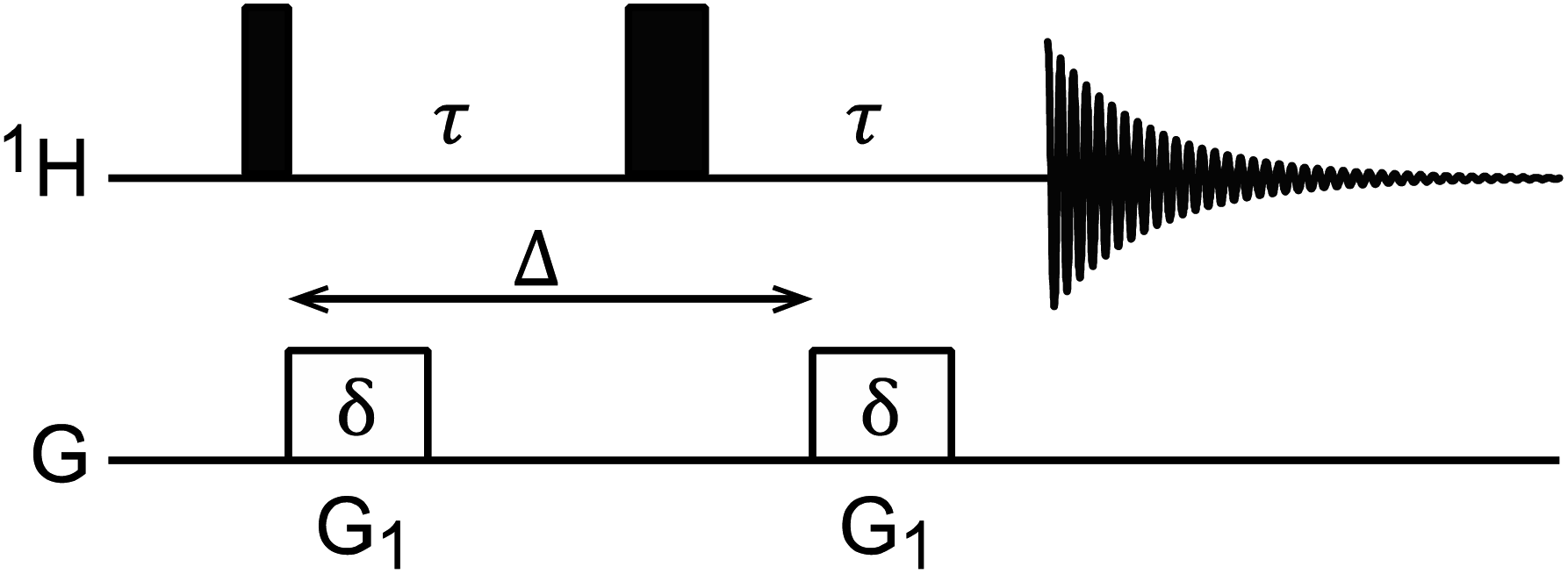
Diffusion ordered spectroscopy (DOSY)
DOSY is a useful NMR technique to measure the diffusion coefficients (D) of molecules.167 The most basic DOSY pulse sequence is shown in Fig. 5.168 A 90° pulse is applied to excite the nuclear spins, followed by the first gradient, which labels the spins with a phase change that depends on their positions in the NMR tube. A 180° pulse is then applied to invert the sign of the phase change, and a second gradient is applied to refocus the signal. When a sample molecule diffuses during the delay period (shown as Δ in Fig. 5), its NMR signals will not be completely refocused by the second gradient, resulting in reduced NMR signal intensity. Therefore, free small molecules that diffuse fast in the sample will experience greater signal attenuation than the NP-bound molecules that diffuse slowly due to the large size of the NP.
 |
| | Fig. 5
1H DOSY pulse sequence.168 The black narrow and wide rectangular-shaped pulses represent 90° and 180° pulses, respectively. The white rectangles represent gradient pulses. Δ is the delay period (i.e. time of diffusion), δ is the gradient duration, and G1 is the gradient strength. | |
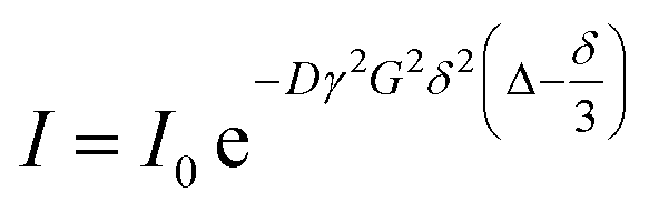
The intensity change from DOSY experiments can be quantitatively described by the Stejskal–Tanner equation:169
| |  | (21) |
where
I is the observed intensity,
I0 is the initial intensity,
D is the diffusion coefficient,
γ is the gyromagnetic ratio,
G is the gradient strength,
δ is the gradient duration, and
Δ is the delay period. To obtain the value of
D, a series of measurements are taken by varying either the gradient strength, the gradient duration, or the delay period and fitting the intensity decay using
eqn (21). 2D DOSY spectra are generated by plotting chemical shifts on one axis and diffusion constants on the other.
170 Each line in the NMR spectrum will give one or more lines in the diffusion dimension at the values corresponding to the diffusion coefficient of the associated species. Therefore, DOSY makes a powerful tool for analyzing mixtures containing more than one ligand–NP species. Moreover, for a spherical molecule, the diffusion coefficient can be used to determine the molecular size using the Stokes–Einstein equation:
| |  | (22) |
where
kB is the Boltzmann constant,
T is the temperature,
η is the viscosity of the solution, and
rH is the hydrodynamic radius of a molecule. Therefore, an estimate of the NP size can be obtained from the value of
D obtained for the bound species.
One very important aspect to notice is that the exchange regimes of a DOSY experiment are defined by the diffusion time (Δ). Considering a simple two-state exchange model where a molecule is in an exchange between states A and B (eqn (9)), the fast exchange regime in the diffusion timescale is defined when Δ ≫ 1/kex (i.e. several exchange events between states A and B occur during Δ), and the slow exchange regime in the diffusion timescale is defined when Δ ≪ 1/kex (i.e. very few exchange events between states A and B occur during Δ).171–173 Therefore, by varying Δ, one can observe the system in either fast or slow exchange in the diffusion timescale. If the exchange is fast in the diffusion timescale, a single population weighted diffusion coefficient will be observed:
where
Dobs is the observed diffusion coefficient, and
pn and
Dn are the fractional population and diffusion coefficient of state n, respectively. If the exchange is slow in the diffusion timescale, two different diffusion coefficients will be observed, resulting in a bi-exponential decay of signal intensity as a function of the varying parameter in the DOSY experiment (
G,
δ, or
Δ in
eqn (21) – see above).
Given that Δ defines the exchange regime in diffusion experiments, DOSY can be applied to exchange systems occurring on a wide range of timescales. However, if Δ ≪ 1/kex and Δω ≫ kex (i.e. the system is in slow exchange in both the diffusion and chemical shift timescales), no change in D will be observed by fitting the intensity of the NMR-visible signal of the free ligand with eqn (21). This limitation, together with the fact that Δ cannot be larger than 1/R2 (to avoid excessive intensity loss during the experiment), hampers the application of DOSY to ligand–NP systems for which R2 ≫ kex.
DOSY experiments have been used to characterize several ligand–NP systems. For example, Hens et al. investigated trioctylphosphine oxide (TOPO) capped colloidal InP nanocrystals using solution NMR.174 From the diffusion coefficient obtained from DOSY measurements and comparing it to the nanocrystal diameter, the authors determined that the broad resonance superimposed on the free TOPO signal was coming from TOPO molecules adsorbed at colloidal nanocrystals. Similarly, Moreels et al. used DOSY measurements to identify the ligands that are tightly bound to the surface of the PbSe nanocrystals.175 In another example, using DOSY, Hassinen et al. determined that octylamines are dynamic ligands for CdSe quantum dots and that free and bound octylamines exhibit fast exchange.176
Saturation transfer methods
When a small molecule is in an exchange between the free and NP-bound states, the large molecular size of the NP increases the R2 of the bound small molecule. The increase in R2 is often large enough to cause broadening of the NMR signal beyond detection level. Saturation transfer experiments achieve indirect detection of the bound state on the spectra of the NMR-visible desorbed state by selective saturation of the NP or the bound state itself. The saturation is then transferred to the visible state via chemical exchange. This section will discuss the two main saturation transfer experiments applied to ligand–NP systems: saturation transfer difference (STD) and dark-state saturation transfer (DEST).
Saturation transfer difference (STD) NMR.
The STD NMR method has been widely used to study ligand–protein interactions.177–180 The standard pulse sequence for 1D 1H STD NMR is shown in Fig. 6a. It involves a train of Gaussian-shaped pulses to achieve the saturation of selected resonances before applying a hard 90° reading pulse. The STD NMR experiment requires taking the difference between an on-resonance spectrum obtained by selectively saturating the 1H signals of the NP and a reference off-resonance spectrum in which the saturation field is moved to a region that does not contain peaks of the NP or the ligand. In the on-resonance experiment, the saturation applied to selective NP resonances is quickly transferred to the other 1H spin on the NP as well as to protons of any ligand bound to the NP surface via spin diffusion (which is highly efficient among 1H spins in high molecular weight systems such as proteins and NPs). Therefore, when bound ligands dissociate into the solution, they cause a decrease in the signal intensity of the free state due to the partial transfer of saturation from the NP-bound state. As a result, when the on-resonance spectrum is subtracted from the off-resonance reference, only signals from ligands that bind to the NP will persist (Fig. 6b).
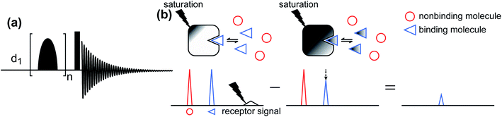 |
| | Fig. 6 (a) Standard pulse sequence for 1D STD NMR. The saturation is achieved by applying a train of n Gaussian-shaped pulses. After the saturation period, a 90° excitation pulse (represented by the rectangular-shaped pulse) is applied. d1 identifies the recycling delay. (b) Schematic representation of the STD NMR protocol. Selective saturation is applied to a receptor proton signal. The saturation is transferred to the entire receptor and to any NMR-invisible attached ligand via spin diffusion. When the ligand dissociates from the receptor, it carries the saturation in the NMR-visible state, reducing the intensity of the observed NMR signal. Therefore, when the saturated spectrum is subtracted from a reference spectrum (acquired in the absence of saturation), only residual signals originating from small molecules that bind to the receptor are visible. | |
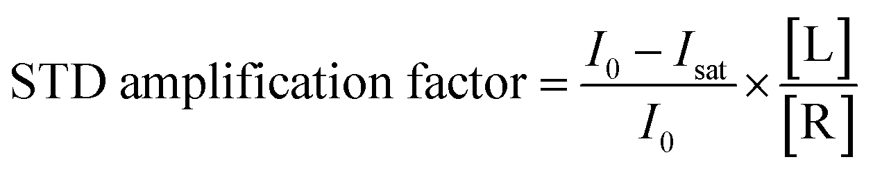
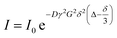
Quantitative interpretation of the STD experiment can be obtained by analyzing the magnitude of the STD effect measured as:
| |  | (24) |
where
I0 and
Isat are the signal intensities in the off- and on-resonance spectrum, respectively. The STD effect is then normalized by multiplying it by the ligand excess, yielding the STD amplification factor.
178| |  | (25) |
where [L] and [R] are the concentrations of ligand and receptor, respectively. A titration curve of the STD amplification factor as a function of the ligand concentration can be fit using a binding isotherm to determine the equilibrium constant for the binding process.
178
STD NMR protocols and theoretical modeling have been extensively developed and tested for screening projects aimed at identifying ligands for protein drug targets.177,181–183 More recently, several STD NMR applications to the investigation of NP adsorption have appeared in the literature. For example, STD NMR has been used to screen libraries of small molecules against NP targets,184,185 to determine the affinities of NP–ligand adducts,184,186 and to investigate the forces driving small molecule adsorption.187 It is important to note that when using the STD NMR for NPs, the concentration of the receptor (noted as [R] in eqn (25)) should be the total concentration of binding sites. As discussed above, when introducing the Langmuir model, this quantity is not easily measurable for NP receptors and introduces ambiguities in the interpretation of the experimental data. To overcome this issue, Zhang et al. used a constant proportional to the surface area of the NP in place of the concentration of the binding sites to calculate the relative STD amplification factor.184 STD NMR can also give structural insight into the adsorption process. For example, by analyzing the pattern of STD amplification factors measured for the 1H nuclei of rhodamine B, it was observed that the small molecule binds to polystyrene NPs via its benzoic acid ring.186
Despite the successful applications described above, a number of factors limit the widespread use of STD NMR in the characterization of sorption equilibria. Indeed, while STD NMR is effective for k−1 > R1 (note that a dissociation rate slower than the longitudinal relaxation would cause the ligand to relax back to equilibrium before returning into the NMR-visible free state), a very large k−1 may result in a population of bound state too low to be detected by the experiment.179 Another limitation of the STD NMR experiment is that the NP must be protonated in order to permit efficient saturation transfer via1H spin diffusion. Such condition hampers the applicability of STD NMR to the analysis of adsorption on metal or metal oxide NPs.
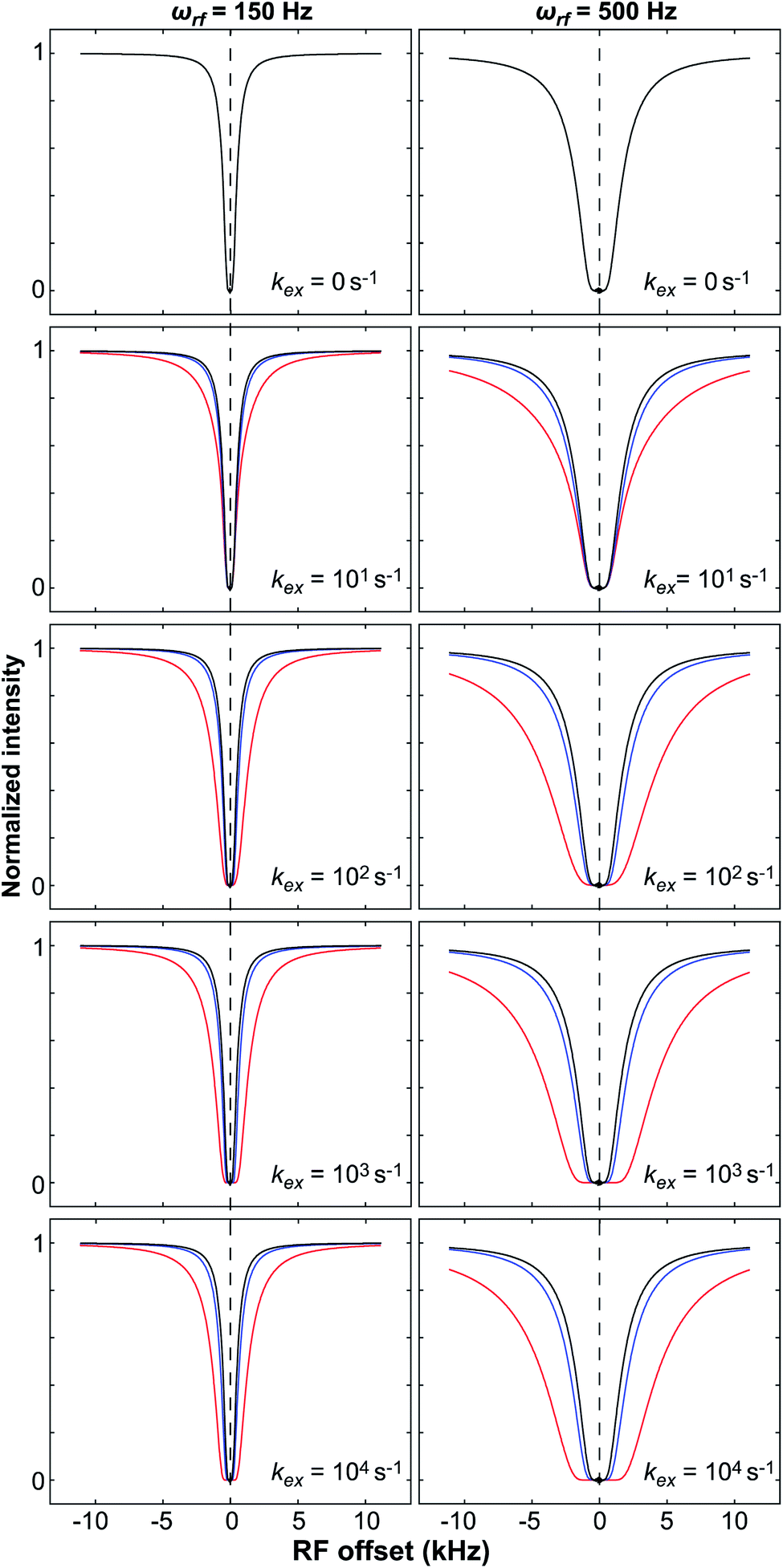
Dark-state exchange saturation transfer (DEST).
The DEST experiment was originally developed to obtain thermodynamic, kinetic, and structural information on the interaction between small, NMR-visible proteins and large aggregates.154,188–190 Later, the application of DEST was expanded to the investigation of ligand–NP interactions.191,192 The DEST experiment takes advantage of the fact that the NMR resonances of the NP-bound state can be saturated selectively by applying a weak radiofrequency (RF) field far off-resonance from the resonances of the free state. Indeed, although broadened out beyond detection level, the bound state resonances are still present within the NMR spectrum. Given their large linewidth, the bound state peaks can be selectively saturated by an RF field positioned at a large offset compared to the resonances of the NMR-visible state. The saturation is then transferred from the bound state to the free state via chemical exchange and observed as a reduction in the signal intensity of free species (Fig. 7). In a typical setup, the DEST experiment is repeated at several RF field offsets to obtain a DEST profile reporting the signal intensity of the NMR-visible state as a function of the offset. The presence of an NMR-invisible bound state in chemical exchange with the NMR-visible free state will be detected as a broadening of the DEST profile compared to the one measured in the absence of NP (Fig. 7). The width of the DEST profile depends on the R2 of the bound state and the strength of the applied RF field, as shown in Fig. 8. The higher the R2 of the bound state and the stronger the RF field, the broader the DEST profile will be.
 |
| | Fig. 7 (a) In the DEST experiment, the NMR-invisible surface-bound species is selectively saturated by an off-resonance RF field. The saturation is then transferred to the visible free species via chemical exchange, resulting in reduced signal intensity. (b) Simulated NMR signals for a free small molecule with R2 = 10 s−1 (black line) and for a NP-bound small molecule with R2 = 100 (blue line) or 1000 s−1 (red line). The broad resonance of the NP-bound state can be selectively saturated by an off-resonance RF. (c) A DEST profile is constructed by plotting the intensity of the NMR-visible peak as a function of the RF offset. The black line is the DEST profile simulated for a small molecule with R2 = 10 s−1 in the absence of exchange. The blue and red lines are the DEST profiles simulated in the presence of exchange with an NP-bound state with R2 = 100 and 1000 s−1, respectively. In all simulations, ωrf = 150 Hz, pA = 0.95, and kex = 600 s−1. Note that, in the absence of exchange, a sharp DEST profile is obtained since saturation of the visible signal is achieved at small RF offsets only. In the presence of exchange with a species with large R2, a broader DEST profile is obtained since saturation of the NP-bound state at large RF offsets is transferred to the NMR-visible state by chemical exchange. | |
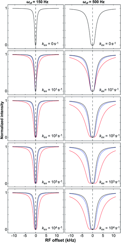 |
| | Fig. 8 Simulated DEST profiles for a two-site exchange equilibrium between the NMR-visible (pA = 0.95 and RA2 = 10 s−1) and NMR-invisible (pB = 0.05) states over a range of kex values (0 to 10000 s−1, top to bottom). RB2 was set to 100 (blue line) or 1000 s−1(red line) to simulate adsorption to a small or large NP, respectively. The DEST curve simulated at kex = 0 s−1 (corresponding to the data obtained in the absence of NP) is colored black. The saturation field strengths are 150 and 500 Hz for the left and right panels, respectively. Note that the DEST experiment is most efficient in detecting ligand–NP adduct with large RB2 that exchange slowly with the desorbed state (kex ≪ RB2 − RA2). In the fast exchange limit, the shape of the DEST profile is no longer dependent from kex. | |
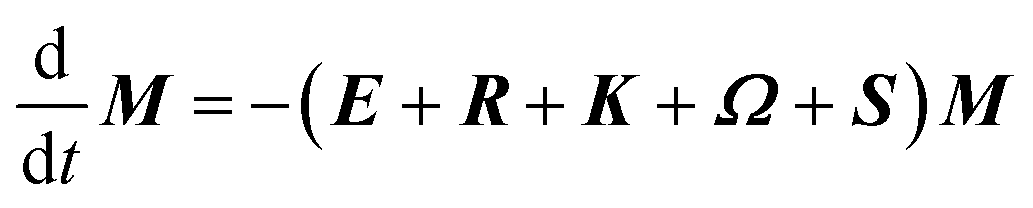
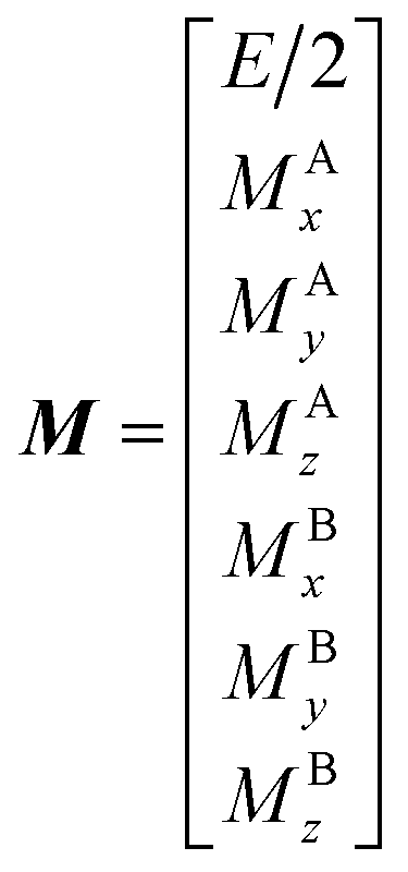
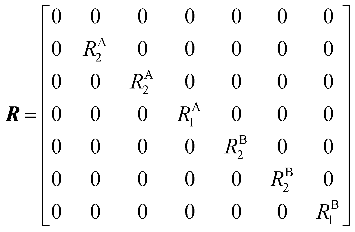
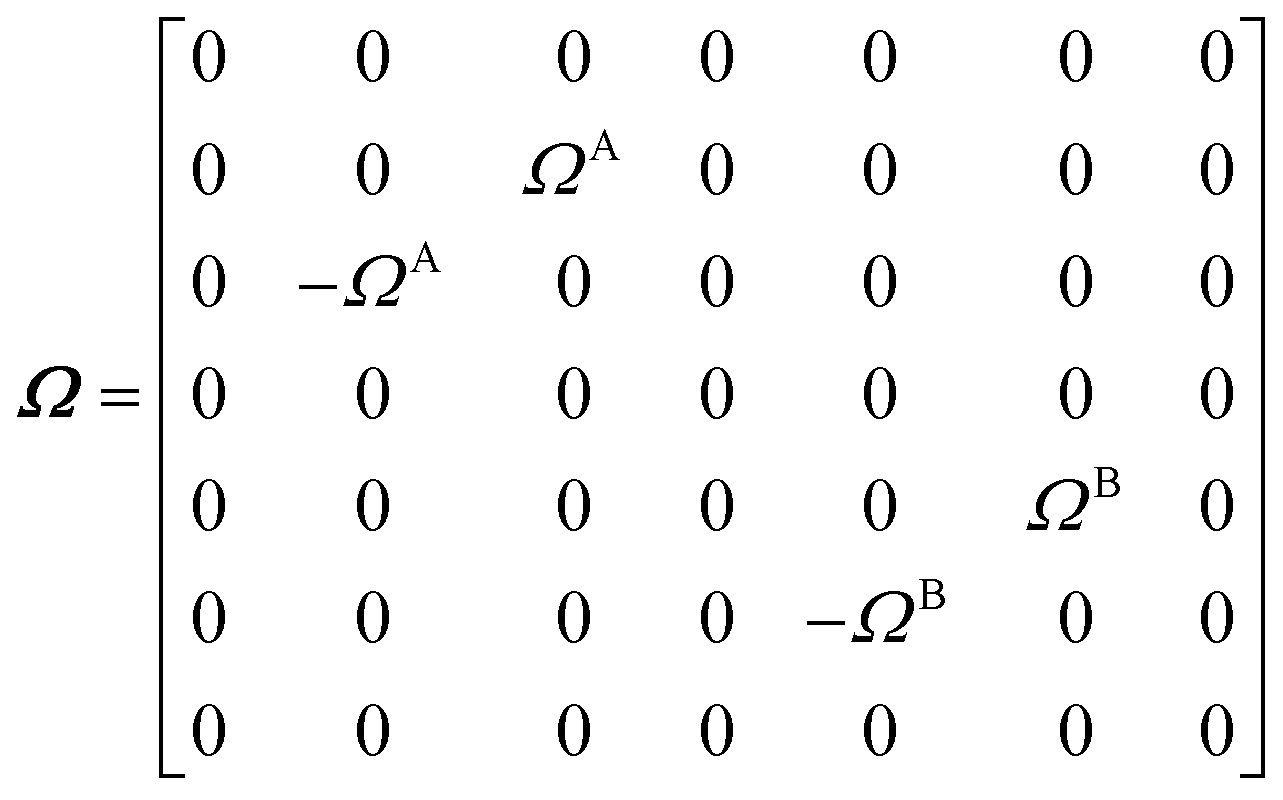
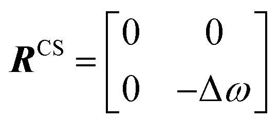
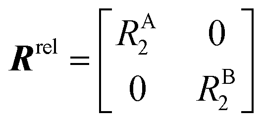
The DEST profile can be modelled using the Bloch–McConnell equation to obtain populations of free and bound states and exchange rates.189 For a two-site exchange system, the signal intensities for different RF offsets can be simulated by solving the following differential equation:
| |  | (26) |
where
M is the matrix representing the magnetization of each state in chemical exchange,
E is the matrix representing the equilibrium magnetization,
R is the matrix representing the relaxation rates of each state,
K is the matrix representing the rate constants for the exchange kinetics,
Ω is the matrix representing the saturation offset, and
S is the matrix representing the saturation field strength.
193 The matrices for each term are shown below:
| | 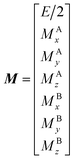 | (27) |
| | 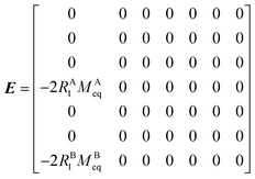 | (28) |
| | 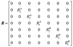 | (29) |
| | 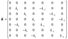 | (30) |
| | 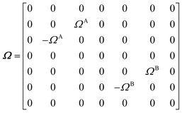 | (31) |
| | 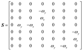 | (32) |
where
E is unity,
Mnk represents the magnetization on the
k-axis of state n,
Ωn represents the difference between the resonance frequency of state n and the frequency of the applied saturation field, and
ωk is the strength of the saturation field applied to the
k-axis.
When modelling a DEST profile, RA1, RA2, ωx, and ωy are usually provided as input parameters and not optimized (note that RA1 and RA2 can be measured experimentally on samples of the ligand prepared without adding the NP). Therefore, data modelling returns RB1, RB2, ΩA, ΩB, k1, and k−1. The thermodynamics of the equilibrium can be calculated from the modelled parameters using the equations:
| |  | (33) |
| |  | (34) |
The DEST experiment is an excellent method for detecting and characterizing large systems that are NMR-invisible due to their fast relaxation rates. Since the DEST experiment uses a relatively high saturation field strength (larger than 100 Hz) to maximize the detection of the NMR-invisible state (Fig. 8), the difference in chemical shift between the states in chemical exchange is usually not resolved154 (note that this is the main difference between DEST and CEST,194 another saturation transfer NMR experiment that uses low saturation field strengths to resolve chemical shift differences between chemical states with similar R2's). Therefore, when modelling DEST profiles, ΩA and ΩB are often considered to be equal in order to reduce the number of variable parameters. Also, it is important to highlight that if the R2 of the bound state is smaller than the applied saturation field, pB and RB2 cannot be determined independently with the DEST experiment alone, and additional experimental data are needed to decorrelate the two parameters.195 Alternatively, the two parameters can be decorrelated by calculating RB2 based on the rotational correlation time of the NP (τNP) that can be estimated by using the average size of the NP and the Stoke–Einstein equation.
DEST can characterize the exchange between a small molecule and a large receptor occurring on the slow timescale (ms–s) at the condition that kex is faster than R1 (which implies that the exchange from free to bound and back to the free state has to occur before the longitudinal magnetization is lost via R1 relaxation). For completeness, it should be mentioned that DEST data can also be acquired for systems exchanging on a fast timescale (kex > 1000 s−1).154 However, as in a fast exchanging system, one single peak is observed with a population-averaged Robs2 (eqn (11)), the R2 of the bound state must be small to avoid the complete loss of the NMR signal.
Compared to STD NMR, the main limitation of DEST is the need to use heteronuclei for the saturation step, which limits its sensitivity and increases the experimental acquisition time. Indeed, when using 1H DEST, the fast 1H spin diffusion can cause unwanted intra and intermolecular magnetization transfers that complicate modelling of the experimental data.189,192 To avoid this issue, several 2D and 1D proton detected pulse sequences were developed to perform 13C or 15N DEST experiments on proteins and small molecules.190,192,196 The pulse sequence used for 1D 13C DEST is shown in Fig. 9. Although less sensitive than STD, the DEST experiment holds the advantage of not requiring a transfer of saturation from the NP to the ligand via spin diffusion, which allows investigation of non-protonated receptors such as metal and metal oxides NPs.
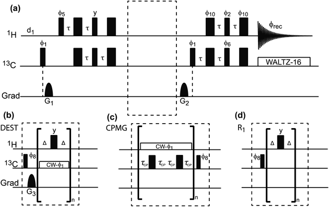 |
| | Fig. 9 (a) Pulse sequences used to measure proton-detected 1D 13C DEST, CPMG, and R1 experiments. Each experiment is measured by inserting the blocks shown in (b)–(d) into the dashed box shown in the double refocused-INEPT based sequence. Full details on the pulse sequences are available in Egner et al.192 In the DEST experiment, CW represents the continuous wave used for saturation. During the saturation period, a train of 180° pulse (represented by the thicker rectangular-shaped pulse) is applied in the 1H channel to remove relaxation artifacts coming from the 1H–13C dipolar interaction. In the CPMG experiment, τCP is a variable parameter that determines the CPMG field (νCPMG = 1/4τCP Hz). The CW applied in the CPMG experiment is for 1H decoupling. The phase cycling employed is: ϕ1 = (x, −x); ϕ2 = 2(x), 2(−x); ϕ5 = 8(x), 8(−x); ϕ6 = 4(y), 4(−y); ϕ8 = (y, −y); ϕ10 = 16(x), 16(−x); ϕrec = 2(x), 4(y), 2(x), 2(y), 4(x), 2(y). The duration and strength of the gradients are as follows: G1, 1 ms, 30 G cm−1; G2, 0.05 ms, 35 G cm−1; G3, 0.1 ms, 40 G cm−1. | |
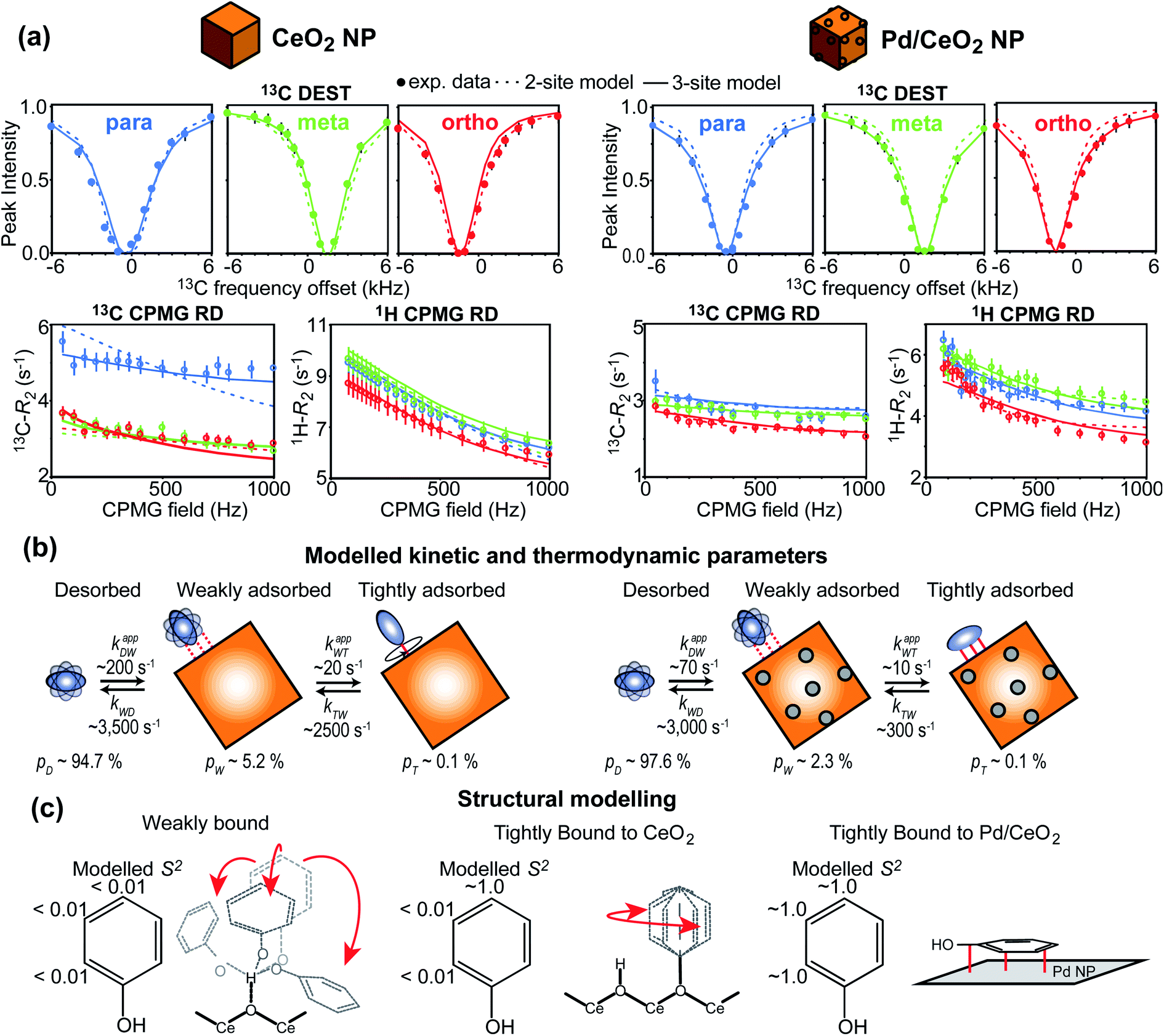
In recent years, several applications of DEST to the investigation of ligand adsorption on NPs were reported. Ceccon et al. determined the kinetics and thermodynamics of adsorption of the huntingtin peptide over titanium(IV) oxide (TiO2) NPs by simultaneous analysis of 15N DEST and ΔR2 (difference in R2 of the free state in the absence and the presence of NP – see below) data.197 Similarly, using 15N DEST, ΔR2, and exchange-induced chemical shift, Hassan et al. characterized the dynamics and exchange kinetics of the interaction between ubiquitin and mercaptosuccinic acid-capped CdTe quantum dots.198 The DEST experiment has also been used to investigate the structures of the surface-bound species. For example, we used 13C DEST in combination with other NMR relaxation methods to characterize not only the kinetics and thermodynamics of binding but also the structure of phenol (PhOH) adsorbed on the surface of ceria (CeO2) and Pd on ceria (Pd/CeO2) NPs.192 With the combination of 1H DEST and molecular dynamics (MD) simulations, Xue et al. determined the adsorption mode of different amino acids on the surface of TiO2 NPs.199
NMR relaxation
NMR relaxation is one of the most prevalent methods to study macromolecular dynamics due to its extreme sensitivity to molecular motions.200–205 Since the overall tumbling and internal motions of a molecule are often significantly perturbed by the surface interaction (e.g., decrease in molecular mobility of the ligand upon binding to NP surface), NMR relaxation makes an ideal method for detecting and characterizing adsorption processes in solution. This section will discuss how relaxation-based NMR methods have been applied to small molecule–NP systems. We will focus our attention on the R1, R2, and relaxation dispersion experiments.
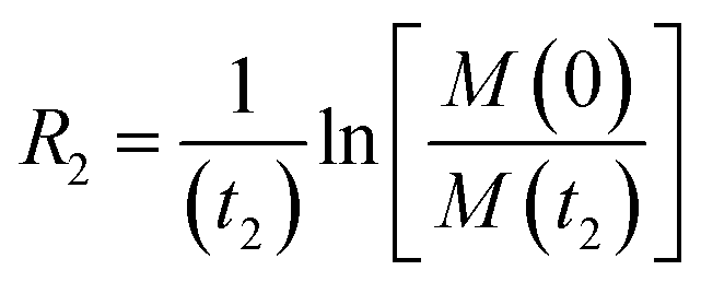
Transverse relaxation (R2).
As discussed above, the transverse relaxation rate of a ligand is enhanced by chemical exchange with an NMR-invisible NP-associated state. Since the increase in R2 of the free ligand reflects the properties of the bound state (e.g., population, binding kinetics, and internal flexibility), the measured transverse relaxation can be used to characterize the ligand–NP interaction. In particular, the relevant observable is the increase in R2 upon addition of NP (ΔR2) measured as:| | | ΔR2 = RNP2 − RnoNP2 = RNP2 − RA2 | (35) |
where RNP2 and RnoNP2 are the R2 values measured for the free ligand NMR signals in the presence and in the absence of the NP, respectively. In the fast exchange regime, ΔR2 = Rllb (eqn (15)) and can be linked to the fractional populations of desorbed and adsorbed species and to their transverse relaxation rates using the formula:| | | ΔR2 = pB(RB2 − RA2) ∼ pBRB2 | (36) |
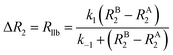
Therefore, RB2 and the concentrations of free and bound ligand (CL and qLS in eqn (3)) can be obtained by modelling ΔR2 data with eqn (36). As discussed above, in the slow exchange regime, if RB2 > k−1, ΔR2 = Rllb = k1 (eqn (17)). However, if the transverse relaxation rate of the NP-bound state is not sufficiently fast to destroy all magnetization (i.e. if RB2 < k−1), then the enhancement to the transverse relaxation rate will be less than k1. In the case pA ≫ pB (which is very common in solution NMR investigation of sorption – see above), it can be shown that:206
| |  | (37) |
which is valid for both the fast and slow timescale regimes. However, it is important to note that in the most common scenario of the intermediate exchange regime, the experimental Δ
R2 is enhanced by
Rex (
eqn (12) and
(13)), and, if the exchange contribution cannot be completely suppressed by the pulse sequence used to measure
R2 (
i.e. using a spinlock field of sufficient strength), the Bloch–McConnell equation should be used to model
Rex into the data analysis (see below).
Although the ΔR2 values are often analyzed in combination with datasets from other NMR experiments (i.e. DEST and relaxation dispersion), a few standalone applications of ΔR2 for quantitative investigation of sorption equilibria are available in the literature. Ceccon et al. have used ΔR2 to investigate the adsorption of ubiquitin on liposome NPs.191 Using the distribution of 15N ΔR2 along the amino acid sequence, they showed that ubiquitin undergoes fast rigid-body rotation about an internal axis while bound to the surface of the NP. In addition, using paramagnetically labeled NPs, they used ΔR2 to measure the dipolar interaction between the protein and the paramagnetic center, which allowed the determination of the ubiquitin residues in direct contact with the NP surface. Xie and Brüschweiler used 13C ΔR2 to investigate how ligand modifications affect binding to silica NPs.207 In particular, they used the fact that in the fast exchange regime pB ∼ ΔR2/RB2 (eqn (36)) to obtain the free energy of adsorption for a variety of ligand–NP interactions. We have shown that, if predicted binding modes are available for a ligand–NP system, a standalone interpretation of ΔR2 can be used to obtain a semi-quantitative analysis of sorption based on the use of scaling factors that depend on the amount of small molecule in each binding mode.208 Using this approach, we determined that functionalization of PhOH with an oxygen at position 2 or 4 greatly enhances adsorption on the Pd or CeO2 component of Pd/CeO2 nanorods, respectively.
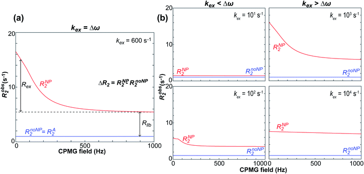
Carr–Purcell–Meiboom–Gill (CPMG) relaxation dispersion (RD).
RD relies on measuring the transverse relaxation at increasing repetition rate of 180° refocusing pulses to progressively suppress the Rex contribution to the R2 of a system in chemical exchange on the intermediate timescale (kex ∼ Δω ≠ 0).154 In CPMG RD, the CPMG field is introduced as a series of refocusing 180° pulses spaced by a constant delay (2τCP) (Fig. 9). As the CPMG field is equal to 1/4τCP, an RD profile can be obtained experimentally by plotting the R2 measured at different τCP values as a function of the CPMG field. Fig. 10a shows an ideal RD profile simulated for the NMR-visible signal of a small molecule in an exchange between the desorbed and NP-adsorbed state on the intermediate timescale. The R2 of such signal will be enhanced compared to the one measured in the absence of NP by both Rex and Rllb:| | | Robs2 = RA2 + ΔR2 = RA2 + Rex + Rllb | (38) |
 |
| | Fig. 10 Simulated CPMG relaxation dispersion curves over a range of kex values. The curves are shown as red solid lines for a two-site sorption equilibrium where the NMR-visible desorbed species is observed. The simulations were obtained with RA2 = 1 s−1, RB2 = 100 s−1, pB = 0.05, and Δω = 600 rad s−1. The RD profile simulated in the absence of exchange between desorbed and adsorbed states (corresponding to the RD profile obtained in the absence of NP) is shown as a blue solid line. In (a) the RD curve for a system in the intermediate exchange regime (kex = Δω) is shown. The Rllb and Rex contributions to ΔR2 are shown as black solid lines. In (b) RD profiles simulated for the slow (kex ≪ Δω, left column) and fast (kex ≫ Δω, right column) exchange regimes are shown. | |
Progressive suppression of Rex by increasing the CPMG field introduces a curvature in the RD profile that plateaus when Rex ∼ 0 s−1 (note that only in this condition the experimental ΔR2 = Rllb).
Fig. 10b shows the RD profiles simulated for two-state sorption equilibria occurring on different timescales. If the exchange is fast or slow on the chemical shift timescale (kex ≫ Δω or kex ≪ Δω, respectively), Rex ∼ 0 s−1 and Robs2 = RA2 + Rllb for any CPMG field. However, within these limits, the shape of the RD profile is very sensitive to the timescale of the equilibrium, and modelling of experimental RD datasets can provide information on the kinetics and thermodynamics of sorption. The R2 at any specific value of τCP can be calculated using the formula:
| | 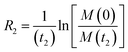 | (39) |
where
M(0) and
M(
t2) are the transverse magnetization calculated for a duration of the CPMG block of 0 and
t2 s, respectively.
M(0) and
M(
t2) are the first elements of vectors
M(0) and
M(
t2), respectively:
| |  | (40) |
| | | M(t2) = (AA*A*A)nM(0) | (41) |
where
MA and
MB represent the transverse magnetizations of states A and B, respectively,
n is the number of CPMG cycles used (see
Fig. 9),
A* the complex conjugate of
A, and
A is given by:
R
is given by:
| | | R = iRCS + Rrel + Rex | (43) |
with
| | 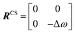 | (44) |
| |  | (45) |
| | 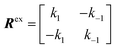 | (46) |
Modelling an RD profile returns RB2, Δω, k1, and k−1 (note that RA2 can be measured experimentally on samples of the ligand prepared without adding the NP). pA and pB can be obtained from the modelled parameters using eqn (33) and (34).
Although CPMG RD is commonly applied to characterize chemical exchange with kex values between 200 and 2000 s−1, the method performs best for processes occurring on the intermediate to slow timescale.154 Indeed, in the intermediate to fast regime, Δω and pB cannot be accurately modelled by a single CPMG data set, and it is common to acquire RD data at multiple static fields and external temperatures to improve the accuracy of modelling.154,209 Also, when possible, it is preferable to measure RD profiles on 1H spins. On conventional NMR spectrometers, the proton channel can sustain higher CPMG fields compared to channels dedicated to heteronuclei, which allows more efficient suppression of Rex for intermediate to fast exchange processes. Also, given the high gyromagnetic ratio, 1H spins tend to have larger Δω, which increases the ability of the RD method to detect and characterize exchange processes with small pB and large kex. A pulse sequence for acquisition of 1D 1H CPMG experiments on small molecule–NP systems is shown in Fig. 11.
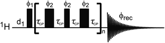 |
| | Fig. 11 PROJECT pulse sequence used for 1H CPMG spectra of small molecules.229 The narrow and wide rectangular-shaped pulses represent 90° and 180° pulses, respectively. The 90° pulse sandwiched between the refocusing CPMG pulses is used to suppress modulation from homonuclear scalar coupling. τCP is a variable parameter that determines the CPMG field (νCPMG = 1/4τCP Hz). The phase cycling employed is: ϕ1 = 2(x), 2(y), 2(−x), 2(−y); ϕ2 = y, −y, y, −y, x, −x, x, −x; ϕrec = 2(x), 2(−x), 2(y), 2(−y). | |
Although CPMG RD has been one of the most popular methods to characterize protein conformational equilibria,210–216 its standalone application to the characterization of ligand–NP systems has been quite limited. Recently, CPMG RD has been combined with DEST, ΔR2, and R1 data to investigate sorption equilibria involving both protein and small molecule ligands.155,192,217
Longitudinal relaxation (R1).
Compared to R2, the longitudinal relaxation is less sensitive to chemical exchange. Therefore, changes in R1 upon adsorption are rarely analyzed. Nonetheless, as an estimate for RB1 is obtained from the analysis of DEST (see above), measuring the R1 of the NMR-visible ligand peaks in the absence (RnoNP1 = RA1) and in the presence (RNP1) of NPs can provide additional experimental restraints for modelling sorption equilibria.
R
1 can be obtained from inversion recovery experiments.218,219 A pulse sequence for the 1D proton-detected 13C R1 experiment applied to small molecule–NP systems is shown in Fig. 9. In the presence of exchange between the free and NP-bound state, the experimental RNP1 of the ligand can be modelled according to the following equation:
| |  | (47) |
where
M(0) and
M(
t2) are the detected magnetizations when the relaxation delay (2
nΔ in
Fig. 9d) is set to 0 and
t2 s, respectively.
M(0) and
M(
t2) are the first elements of vectors
M(0) and
M(
t2), respectively:
| |  | (48) |
Here,
MA and
MB represent the initial magnetizations of states A and B, respectively,
A* represents the complex conjugate of
A, and
A is given by:
where
R is given by the summation:
with
| |  | (52) |
| |  | (53) |
Modelling the ligand–NP adduct.
In the sections above, we have discussed how modelling DEST, RD, R1, and/or R2 data measured for the NMR-visible signals of a free ligand in the presence of chemical exchange with a NP-bound state returns the thermodynamic (pA and pB) and kinetic (k1 and k−1) parameters of sorption. In addition, such analysis returns information on the structure and dynamics of the surface-bound species encoded in the modelled RB1 and RB2 values. Indeed, when the exchange contribution is completely suppressed, NMR relaxation is induced by the modulation of magnetic interactions caused by molecular motions occurring on the ps–ns timescale. In the case of spin-half nuclei in a diamagnetic system, the relevant magnetic interactions are dipolar couplings and chemical shift anisotropy (CSA).
For an isolated 1H–13C (or 1H–15N) bond vector, the 13C (or 15N) R1 and R2 are linked to the molecular dynamics using the model-free method developed by Lipari and Szabo:220,221
| |  | (54) |
| |  | (55) |
where
| |  | (56) |
| |  | (57) |
Here,
μ0 is the magnetic permeability, ℏ is the reduced Planck's constant,
γn is the gyromagnetic ratio of the n nucleus,
r is the internuclear bond distance, and Δ
σ is the chemical shift anisotropy.
J(
ω) represents the spectral density function which describes how much local field is oscillating at the given frequency:
| | 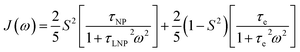 | (58) |
where
S2 is a generalized order parameter representing the spatial restriction of the internal motion,
τLNP is the correlation time of the ligand in a rigid interaction with the NP, and
τe is the effective correlation time of the C–H (or N–H) bond vector given by:
191| |  | (59) |
| |  | (60) |
where
τNP and
τloc are the correlation time of the NP and of the local motion, respectively. In the model-free approach, if the motion of the C–H bond vector is restricted (
i.e. the C–H bond is rigidly attached to the NP surface),
S2 ∼ 1 and the overall tumbling of the NP and binding kinetics are the only contribution to relaxation (
i.e.,
τLNP is the only correlation time modulating the magnetic interactions –
eqn (58)). On the other hand, if the C–H bond vector is highly flexible,
S2 ∼ 0 and relaxation is determined by both
τLNP and
τloc.
Modelling 13C and 15N relaxation rates using the model-free approach was used to investigate the molecular dynamics of PhOH bound to CeO2 and Pd/CeO2 NPs192,208 and of the protein ubiquitin adsorbed on liposome NPs.191 However, it is important to notice that eqn (54)–(60) only apply to the spin-half heteronuclei covalently attached to single hydrogen (i.e. protein backbone amides, CH groups in aromatic rings, etc.), and more complex models are required for more complex systems.
Combining solution NMR experiments
Several solution NMR experiments have been described above that investigate chemical exchange processes occurring on different timescales. In particular, chemical shift analysis is very powerful for characterizing fast chemical exchange, CPMG RD is particularly suited for intermediate to slow exchange, while saturation transfer methods (STD and DEST) and the analysis of peak intensities work best for processes in the slow exchange regime. In addition to these methods, analysis of DOSY, ΔR1 and ΔR2 experiments can report on the chemical exchange between desorbed and NP-adsorbed states on a broad range of timescales (Fig. 12). Although using these methods as standalone techniques can provide important insight into sorption equilibria, the utility of combining two or more NMR experiments sensitive to different timescales for investigating surface adsorption was demonstrated in several applications. Indeed, adsorption on a heterogeneous surface is often a complex process involving multiple intermediate states and adsorbed species in chemical exchange (among themselves and with the desorbed state) on different timescales, and the combined analysis of different NMR observables can help to deconvolute the contribution of each elementary step to surface adsorption. For example, Libich et al. investigated the interaction of the polypeptide amyloid β (Aβ40) with the molecular chaperone GroEL by using a combination of 15N ΔR2, 15N DEST, 15N CPMG RD, and exchange-induced chemical shift change analysis.217 They showed that since these methods depend differently on the kinetics and thermodynamics of adsorption, their combined analysis increased the stability of data modelling and the precision of the fitted parameters. In addition, by combining 15N ΔR2, 13C and 15N DEST, and 1H, 13C, and 15N CPMG RD, Libich et al. investigated the chaperonin activity of GroEL, demonstrating that the molecular machinery accelerates the interconversion between the native and partially folded states of a triple mutant of the Fyn SH3 domain.222 Another series of studies explored the combination of 1H R1 and R2 for investigating sorption in porous materials.223 It was found that the 1H R2/R1 ratio of ligands in saturated porous media provides information on the residence time of the NMR-visible small molecule inside the pore and on the energy of adsorption.224
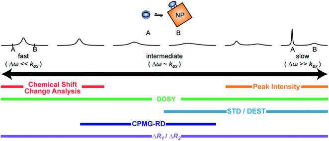 |
| | Fig. 12 Summary of solution NMR experiments for investigating sorption equilibria occurring on different exchange regimes. | |
In the following section, we highlight how the combination of 13C R1, 13C R2, 13C DEST, and 1H and 13C CPMG RD was used to investigate small molecule–NP sorption with atomic resolution. In particular, using the interaction between PhOH and Pd/CeO2 nanocubes as the model system, we will illustrate the combined use of multiple NMR methods to obtain kinetic, thermodynamic, and structural information on adsorption/desorption equilibria involving multiple elementary steps occurring on multiple timescales.
Application to the PhOH–Pd/CeO2 system
Pd/CeO2 NPs catalyze the hydrogenation of PhOH under mild reaction conditions (1 bar H2 at room temperature) more efficiently than other Pd-based catalysts.225 However, it is unclear whether the outstanding performance of Pd/CeO2 is due to a higher dispersion of the Pd catalyst, better adsorption of PhOH on the catalyst surface, beneficial electronic effects of ceria on the supported metal, or a direct contribution of ceria in catalysis via H2 spillover. To help address this question, in the last few years, we conducted a series of studies aimed at characterizing the adsorption of PhOH on Pd/CeO2 NPs by solution NMR.155,192,208,226
Initially, we focused on studying the binding of PhOH onto bare CeO2 NPs of cubic morphology using 1H DEST and 1H CPMG RD.155 We noticed that the data could not be modelled using a two-site exchange mechanism and that expansion of the Bloch–McConnell matrices to account for the existence of two adsorbed species in chemical exchange with the desorbed state was required in order to fully reproduce the 1H DEST profile. However, due to the high sensitivity of 1H DEST to spin diffusion that overemphasizes contributions from surface-bound species and complications in modelling 1H relaxation, an accurate determination of the kinetic, thermodynamic, and structural parameters of sorption was not obtained in this initial study.
In a follow-up study, we combined 1H and 13C CPMG RD, 13C DEST, and 13C R1 experiments to investigate the adsorption of PhOH on CeO2 and Pd/CeO2 NPs of cubic morphology.192 Consistent with our preliminary investigation using 1H DEST, modelling of the data required a two-step adsorption process in which the desorbed species is in equilibrium with tightly adsorbed PhOH via a weakly associated intermediate state (Fig. 13). It is important to note that simultaneous analysis of all datasets was key to the determination of the two-step binding mechanism. Indeed, a one-step binding model was sufficient to describe the 1H CPMG RD, 13C DEST, and 13C R1 (but not the 13C CPMG RD) measured for PhOH–CeO2, or the 1H and 13C CPMG RD and 13C R1 (but not the 13C DEST) measured for PhOH–Pd/CeO2 (Fig. 13a). Removing spin-diffusion artifacts from the DEST experiment allowed for accurate modelling of the kinetics and thermodynamics of adsorption as well as for determination of the 13C R1 and R2 values for PhOH in the NP-associated states (Fig. 13b). Next, we used the modelled R1 and R2 to calculate the order parameter for each C–H bond in the weakly and tightly associated state by eqn (54)–(60) (Fig. 13c). Analysis of the S2 values indicated that irrespective of the NP, all C–H groups are highly mobile in the weakly associated state (S2 < 0.01), which suggested that this intermediate species consists of PhOH hydrogen-bonded to the CeO2 component of the NP (Fig. 13c, left). On the other hand, we noticed that the S2 values obtained for PhOH tightly associated with CeO2 are position-dependent, with very low S2 values (<0.01) for the ortho and meta positions, and S2 ∼ 1 for the para position. This S2 trend (which is linked to the high 13C R2 measured for the para carbon – Fig. 13a) revealed that while the ortho and meta C–H groups reorient fast relative to the external magnetic field, the para C–H bond reorients with the same correlation time as the NP (see eqn (58)). These considerations brought us to conclude that PhOH associates tightly to CeO2 by inserting the O atom into O-vacancies present on the NP surface. Indeed, the latter interaction mode keeps the para C–H group rigid with respect to the NP surface while allowing fast reorientation of the meta and ortho C–H bonds (Fig. 13c, middle). Finally, the modelling of the relaxation rates returned an S2 ∼ 1 for all C–H bonds of PhOH tightly associated with Pd/CeO2. Such observation indicated that the molecule is rigidly attached to the NP and confirmed a “flat” binding of PhOH to Pd hypothesized by ab initio calculations (Fig. 13c, right).227 In the same work, we have tested the proposed binding models by reacquiring the NMR data in the presence of 20 mM inorganic phosphate, which binds strongly to CeO2 but does not interact with Pd.228 We found that the addition of phosphate reduced the population of PhOH weakly bound to CeO2 and Pd/CeO2, and completely abolished the interaction of PhOH with O-vacancies on CeO2. However, the population and exchange kinetics of PhOH tightly bound to Pd/CeO2 were unaffected by the presence of phosphate, confirming that the tight adsorption of PhOH on Pd/CeO2 is mediated by contacts between PhOH and the Pd component of the NP.
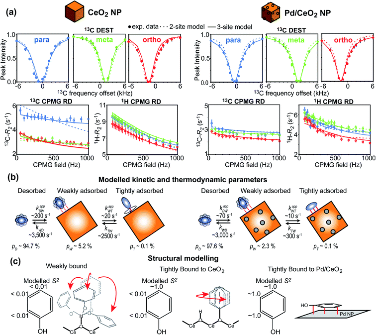 |
| | Fig. 13 Combined analysis of 13C R1, 13C R2, 13C DEST, and 1H and 13C CPMG RD experiments on the PhOH–Pd/CeO2 system. (a) 13C DEST (saturation field strength = 1 kHz) and 1H and 13C CPMG RD profiles of PhOH in the presence of 1 wt% CeO2 (left) and 1 wt% Pd/CeO2 (right) NPs. Data were collected at 800 MHz. Experimental data for the para, meta, and ortho C–H bonds are represented in blue, green, and red circles, respectively. The dotted and solid lines represent the best fit to a two-site and three-site exchange model, respectively. (b) Modelled kinetic and thermodynamic parameters for PhOH adsorption on CeO2 (left) and Pd/CeO2 (right) NPs. PhOH is a blue oblate, CeO2 is an orange square, and Pd sites are gray spheres. (c) Structural modelling of PhOH adsorbed on the CeO2 and Pd/CeO2 surface. The order parameter (S2) obtained for each C–H group is shown. Adapted from Egner et al.192 | |
Finally, in order to address the possible direct involvement of CeO2 in catalytic conversion of PhOH, we compared the kinetics of substrate hydrogenation measured in the presence and in the absence of 20 mM phosphate with the adsorption data obtained by solution NMR. The rationale for this comparison was that reaction rates are proportional to the concentration of active substrate–catalyst complex in solution. Therefore, we expected the reaction rate to be reduced in the presence of phosphate if catalysis is mediated by interactions between PhOH and CeO2 (Fig. 14). The results of our experiment confirmed this scenario and revealed an active role for the support in catalytic hydrogenation of PhOH by Pd/CeO2.
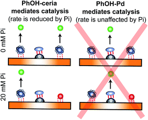 |
| | Fig. 14 Graphic representation of how the direct participation of CeO2 in catalysis was revealed by the addition of inorganic phosphate (Pi). PhOH is a blue oblate, the product of the reaction (cyclohexanone or cyclohexanol) is a green circle, the CeO2 surface is shown as an orange rectangle, the Pd site is a gray half sphere, and Pi is a red circle. The NMR data revealed that while the addition of 20 mM Pi reduced the population of weakly bound PhOH–CeO2 intermediate by ∼50%, it did not affect the population and exchange kinetics of PhOH tightly bound to Pd. Since the rate of PhOH hydrogenation catalyzed by Pd/CeO2 is also reduced by ∼50% by the addition of 20 mM Pi, the results reported in Egner et al.192 suggest that the weak PhOH–CeO2 interaction is catalytically relevant. | |
Conclusions
As applications of NP catalysts continue to expand, understanding sorption equilibria has become of utmost importance since the efficiency and selectivity of NP catalysis are highly dependent on the interactions that substrates, intermediates, and products establish with the NP surface. Over recent years, solution NMR spectroscopy is emerging as a powerful method for detecting and characterizing small molecule–NP interactions due to its exceptional sensitivity to molecular motions and capability of observing dynamic processes over a wide range of timescales. Through this comprehensive review of various solution NMR techniques for characterizing small molecule–NP interactions, we illustrated procedures for stable NMR sample preparation of insoluble NPs, introduced theoretical and practical aspects of the relevant NMR experiments, discussed how the combined analysis of multiple NMR methods can provide mechanistic insight into sorption equilibria involving multiple elementary steps, and reviewed a number of practical applications. We believe solution NMR spectroscopy has a bright future ahead in the investigation of ligand–NP interactions, and we expect it to become a crucial investigative tool for the development of new generations of heterogeneous catalysts.
Conflicts of interest
There are no conflicts to declare.
Acknowledgements
We thank Dr Igor Slowing for critical reading. This work was supported by funds from NIGMS R35GM133488 (to V. V.).
References
- F. Raimondi, G. G. Scherer, R. Kötz and A. Wokaun, Angew. Chem., Int. Ed., 2005, 44, 2190–2209 CrossRef CAS PubMed.
- S. E. Lohse and C. J. Murphy, J. Am. Chem. Soc., 2012, 134, 15607–15620 CrossRef CAS PubMed.
- M. Gharibi, F. T. Zangeneh, F. Yaripour and S. Sahebdelfar, Appl. Catal., A, 2012, 443–444, 8–26 CrossRef CAS.
- X. Sun, Y. Zhang, G. Chen and Z. Gai, Energies, 2017, 10, 345 CrossRef.
- D. P. Cormode, L. Gao and H. Koo, Trends Biotechnol., 2018, 36, 15–29 CrossRef CAS PubMed.
- B. Yang, Y. Chen and J. Shi, Adv. Mater., 2019, 31, 1901778 CrossRef PubMed.
- W. Lin, J. Walter, A. Burger, H. Maid, A. Hirsch, W. Peukert and D. Segets, Chem. Mater., 2015, 27, 358–369 CrossRef CAS.
- M. P. de Haan, N. Balakrishnan, A. R. Kuzmyn, G. Li, H. M. Willemen, G. Seide, G. C. H. Derksen, B. Albada and H. Zuilhof, Langmuir, 2021, 37(4), 1446–1455 CrossRef CAS PubMed.
- J. H. Kim, B. J. Cha, Y. D. Kim and H. O. Seo, Adv. Powder Technol., 2020, 31, 816–826 CrossRef CAS.
- K. Sepideh, M. N. Lotfollahi and A. Shahrabadi, Pet. Chem., 2019, 59, 1201–1206 CrossRef.
- M. Mahmoudi, I. Lynch, M. R. Ejtehadi, M. P. Monopoli, F. B. Bombelli and S. Laurent, Chem. Rev., 2011, 111, 5610–5637 CrossRef CAS PubMed.
- Y. Randika Perera, R. A. Hill and N. C. Fitzkee, Isr. J. Chem., 2019, 59, 962–979 CrossRef CAS PubMed.
- Á. I. López-Lorente and B. Mizaikoff, TrAC, Trends Anal. Chem., 2016, 84, 97–106 CrossRef.
- H. Joshi, P. S. Shirude, V. Bansal, K. N. Ganesh and M. Sastry, J. Phys. Chem. B, 2004, 108, 11535–11540 CrossRef CAS.
- I. Langmuir, J. Am. Chem. Soc., 1916, 38, 2221–2295 CrossRef CAS.
- I. Langmuir, J. Am. Chem. Soc., 1917, 39, 1848–1906 CrossRef CAS.
- I. Langmuir, J. Am. Chem. Soc., 1918, 40, 1361–1403 CrossRef CAS.
- H. Swenson and N. P. Stadie, Langmuir, 2019, 35, 5409–5426 CrossRef CAS PubMed.
-
A. Ben-Naim, in Cooperativity and Regulation in Biochemical Processes, Springer, Boston, MA, 2001, pp. 25–49, DOI:10.1007/978-1-4757-3302-0_2.
- O. Hamdaoui and E. Naffrechoux, J. Hazard. Mater., 2007, 147, 381–394 CrossRef CAS PubMed.
- M. A. Al-Ghouti and D. A. Da'ana, J. Hazard. Mater., 2020, 393, 122383 CrossRef CAS PubMed.
- S. Azizian, S. Eris and L. D. Wilson, Chem. Phys., 2018, 513, 99–104 CrossRef CAS.
- T. Chen, T. Da and Y. Ma, J. Mol. Liq., 2021, 322, 114980 CrossRef CAS.
- S. Lagergren, K. Sven. Vetenskapsakad. Handl., 1898, 24, 1–39 Search PubMed.
- G. Blanchard, M. Maunaye and G. Martin, Water Res., 1984, 18, 1501–1507 CrossRef CAS.
- D. S. Karpovich and G. J. Blanchard, Langmuir, 1994, 10, 3315–3322 CrossRef CAS.
- B. M. DeVetter, P. Mukherjee, C. J. Murphy and R. Bhargava, Nanoscale, 2015, 7, 8766–8775 RSC.
- J. W. Kim, B. Son, H. Yu, H. M. Park and Y.-S. Lee, Surf. Interface Anal., 2014, 46, 193–196 CrossRef CAS.
-
M. H. Engelhard, T. C. Droubay and Y. Du, in Encyclopedia of Spectroscopy and Spectrometry, ed. J. C. Lindon, G. E. Tranter and D. W. Koppenaal, Academic Press, Oxford, 3rd edn, 2017, pp. 716–724, DOI:10.1016/B978-0-12-409547-2.12102-X.
- H. Häkkinen, Nat. Chem., 2012, 4, 443–455 CrossRef PubMed.
- A. Kühnle, T. R. Linderoth, B. Hammer and F. Besenbacher, Nature, 2002, 415, 891–893 CrossRef PubMed.
- L. B. Casabianca, Solid State Nucl. Magn. Reson., 2020, 107, 101664 CrossRef CAS PubMed.
- S. K. Davidowski and G. P. Holland, Langmuir, 2016, 32, 3253–3261 CrossRef CAS PubMed.
- T. Gutmann, A. Grünberg, N. Rothermel, M. Werner, M. Srour, S. Abdulhussain, S. Tan, Y. Xu, H. Breitzke and G. Buntkowsky, Solid State Nucl. Magn. Reson., 2013, 55–56, 1–11 CrossRef CAS PubMed.
- L. R. Becerra, C. B. Murray, R. G. Griffin and M. G. Bawendi, J. Chem. Phys., 1994, 100, 3297–3300 CrossRef CAS.
- G. P. Holland, R. Sharma, J. O. Agola, S. Amin, V. C. Solomon, P. Singh, D. A. Buttry and J. L. Yarger, Chem. Mater., 2007, 19, 2519–2526 CrossRef CAS.
- W. Lin, T. Insley, M. D. Tuttle, L. Zhu, D. A. Berthold, P. Král, C. M. Rienstra and C. J. Murphy, J. Phys. Chem. C, 2015, 119, 21035–21043 CrossRef CAS PubMed.
- J. M. Carnerero, A. Sánchez-Coronilla, E. I. Martín, A. Jimenez-Ruiz and R. Prado-Gotor, Phys. Chem. Chem. Phys., 2017, 19, 22121–22128 RSC.
- L. Yu and N. Li, Langmuir, 2016, 32, 5510–5518 CrossRef CAS PubMed.
- M. Khosravi and S. Azizian, J. Ind. Eng. Chem., 2014, 20, 2561–2567 CrossRef CAS.
- M. Khosravi, B. Yahyaei and S. Azizian, J. Dispersion Sci. Technol., 2014, 35, 1135–1142 CrossRef CAS.
- Y. Wang and Y. Ni, Talanta, 2014, 119, 320–330 CrossRef CAS PubMed.
- T. Zhao, M. Fang, Z. Tang, X. Zhao, F. Xie, F. Wu and J. P. Giesy, Environ. Sci. Pollut. Res., 2019, 26, 21463–21474 CrossRef CAS PubMed.
- S. Jafari, S. Azizian and B. Jaleh, Colloids Surf., A, 2011, 384, 618–623 CrossRef CAS.
- S. D. Roy, M. Ghosh and J. Chowdhury, Spectrochim. Acta, Part A, 2015, 151, 796–806 CrossRef CAS PubMed.
- S. Dutta Roy, M. Ghosh and J. Chowdhury, J. Raman Spectrosc., 2015, 46, 451–461 CrossRef CAS.
- H. Yang, W. Zhang, S. Athukorale, Z. Liu, S. Zou, B. Donnadieu, Z. Wang and D. Zhang, J. Phys. Chem. C, 2020, 124, 686–692 CrossRef CAS.
- I. Blakey, T. L. Schiller, Z. Merican and P. M. Fredericks, Langmuir, 2010, 26, 692–701 CrossRef CAS PubMed.
- K. Siriwardana, B. C. N. Vithanage, S. Zou and D. Zhang, Anal. Chem., 2017, 89, 6686–6694 CrossRef CAS PubMed.
- J. X. Xu, K. Siriwardana, Y. Zhou, S. Zou and D. Zhang, Anal. Chem., 2018, 90, 785–793 CrossRef CAS PubMed.
- C.-C. You, M. De, G. Han and V. M. Rotello, J. Am. Chem. Soc., 2005, 127, 12873–12881 CrossRef CAS PubMed.
- S. Pandit and M. De, J. Phys. Chem. C, 2017, 121, 600–608 CrossRef CAS.
- M. Park, D. P. Salem, D. Parviz, X. Gong, K. S. Silmore, T. T. S. Lew, D. T. Khong, M. C.-Y. Ang, S.-Y. Kwak, M. B. Chan-Park and M. S. Strano, Nano Lett., 2019, 19, 7712–7724 CrossRef CAS PubMed.
- X. Leng, K. Starchev and J. Buffle, Langmuir, 2002, 18, 7602–7608 CrossRef CAS.
- L. M. Demers, C. A. Mirkin, R. C. Mucic, R. A. Reynolds, R. L. Letsinger, R. Elghanian and G. Viswanadham, Anal. Chem., 2000, 72, 5535–5541 CrossRef CAS PubMed.
- Y.-K. Gong, K. Nakashima and R. Xu, Langmuir, 2000, 16, 8546–8548 CrossRef CAS.
- D. Singappuli-Arachchige, T. Kobayashi, Z. Wang, S. J. Burkhow, E. A. Smith, M. Pruski and I. I. Slowing, ACS Catal., 2019, 9, 5574–5582 CrossRef CAS.
- D. Singappuli-Arachchige and I. I. Slowing, J. Chem. Phys., 2020, 152, 034703 CrossRef CAS PubMed.
- H. A. Al-Abadleh and V. H. Grassian, Langmuir, 2003, 19, 341–347 CrossRef CAS.
- B. Torun, C. Kunze, C. Zhang, T. D. Kühne and G. Grundmeier, Phys. Chem. Chem. Phys., 2014, 16, 7377–7384 RSC.
- S. E. Collins, M. A. Baltanás and A. L. Bonivardi, J. Phys. Chem. B, 2006, 110, 5498–5507 CrossRef CAS PubMed.
- M.-Y. He and J. G. Ekerdt, J. Catal., 1984, 87, 381–388 CrossRef CAS.
- R. Narayanan and M. A. El-Sayed, J. Phys. Chem. B, 2005, 109, 4357–4360 CrossRef CAS PubMed.
- J. Petroski and M. A. El-Sayed, J. Phys. Chem. A, 2003, 107, 8371–8375 CrossRef CAS.
- J.-W. Park and J. S. Shumaker-Parry, J. Am. Chem. Soc., 2014, 136, 1907–1921 CrossRef CAS PubMed.
- F. Zhang, W. Ma, Y. Jiao, J. Wang, X. Shan, H. Li, X. Lu and S. Meng, ACS Appl. Mater. Interfaces, 2014, 6, 22359–22369 CrossRef CAS PubMed.
- I. A. Mudunkotuwa, A. A. Minshid and V. H. Grassian, Analyst, 2014, 139, 870–881 RSC.
- F. Porta, Ž. Krpetić, L. Prati, A. Gaiassi and G. Scarì, Langmuir, 2008, 24, 7061–7064 CrossRef CAS PubMed.
- N. Kumar, S. Thomas, R. B. Tokas and R. J. Kshirsagar, Spectrochim. Acta, Part A, 2014, 118, 614–618 CrossRef CAS PubMed.
- A. Susarrey-Arce, R. M. Tiggelaar, J. G. E. Gardeniers, A. van Houselt and L. Lefferts, J. Phys. Chem. C, 2015, 119, 24887–24894 CrossRef CAS.
- S. Jayalath, S. C. Larsen and V. H. Grassian, Environ. Sci.: Nano, 2018, 5, 2162–2171 RSC.
- M. F. Atitar, R. Dillert and D. W. Bahnemann, J. Phys. Chem. C, 2017, 121, 4293–4303 CrossRef CAS.
- X. Zhang, L. Chen, L. Yuan, R. Liu, D. Li, X. Liu and G. Ge, Langmuir, 2019, 35, 5770–5778 CrossRef CAS PubMed.
- B. Botka, A. J. McQuillan, M. Krasowska and D. A. Beattie, Langmuir, 2019, 35, 10734–10743 CrossRef CAS PubMed.
- G. Chong, E. D. Laudadio, M. Wu, C. J. Murphy, R. J. Hamers and R. Hernandez, J. Phys. Chem. C, 2018, 122, 28393–28404 CrossRef CAS.
- M. Osawa, K.-I. Ataka, K. Yoshii and Y. Nishikawa, Appl. Spectrosc., 1993, 47, 1497–1502 CrossRef CAS.
- N. Kumar, S. Thomas, R. B. Tokas and R. J. Kshirsagar, Spectrochim. Acta, Part A, 2014, 129, 359–364 CrossRef CAS PubMed.
- S. Chakrabarty, S. Maity, D. Yazhini and A. Ghosh, Langmuir, 2020, 36, 11255–11261 CrossRef CAS PubMed.
- H. S. Kim, S. J. Lee, N. H. Kim, J. K. Yoon, H. K. Park and K. Kim, Langmuir, 2003, 19, 6701–6710 CrossRef CAS.
- A. Beaussart, L. Petrone, A. Mierczynska-Vasilev, A. J. McQuillan and D. A. Beattie, Langmuir, 2012, 28, 4233–4240 CrossRef CAS PubMed.
- A. G. Young and A. J. McQuillan, Langmuir, 2009, 25, 3538–3548 CrossRef CAS PubMed.
- F. Roncaroli and M. A. Blesa, J. Colloid Interface Sci., 2011, 356, 227–233 CrossRef CAS PubMed.
- S. J. Hug and B. Sulzberger, Langmuir, 1994, 10, 3587–3597 CrossRef CAS.
- F. Roncaroli and M. A. Blesa, J. Coord. Chem., 2010, 63, 2488–2497 CrossRef CAS.
- F. Roncaroli and M. A. Blesa, Phys. Chem. Chem. Phys., 2010, 12, 9938–9944 RSC.
- S. Jayalath, H. Wu, S. C. Larsen and V. H. Grassian, Langmuir, 2018, 34, 3136–3145 CrossRef CAS PubMed.
- F. Roncaroli, E. D. Martínez, G. J. A. A. Soler-Illia and M. A. Blesa, J. Phys. Chem. C, 2013, 117, 15026–15034 CrossRef CAS.
- J. Tofan-Lazar and H. A. Al-Abadleh, J. Phys. Chem. A, 2012, 116, 10143–10149 CrossRef CAS PubMed.
- S. Soldoozy, A. Trinh, J. D. Kubicki and H. A. Al-Abadleh, Langmuir, 2020, 36, 4299–4307 CrossRef CAS PubMed.
- M. A. Sabur and H. A. Al-Abadleh, Can. J. Chem., 2015, 93, 1297–1304 CrossRef CAS.
- A. Aguirre, C. L. A. Berli and S. E. Collins, Catal. Today, 2017, 283, 127–133 CrossRef CAS.
- J. L. Marsh, A. E. Wayman, N. M. Smiddy, D. J. Campbell, J. C. Parker, W. B. Bosma and E. E. Remsen, Langmuir, 2017, 33, 13224–13233 CrossRef CAS PubMed.
- R. Fritzsch, S. Hume, L. Minnes, M. J. Baker, G. A. Burley and N. T. Hunt, Analyst, 2020, 145, 2014–2024 RSC.
- A. L. Le Sueur, R. E. Horness and M. C. Thielges, Analyst, 2015, 140, 4336–4349 RSC.
- P. M. Donaldson and P. Hamm, Angew. Chem., Int. Ed., 2013, 52, 634–638 CrossRef CAS PubMed.
- H. Bian, J. Li, H. Chen, K. Yuan, X. Wen, Y. Li, Z. Sun and J. Zheng, J. Phys. Chem. C, 2012, 116, 7913–7924 CrossRef CAS.
- A. Ghosh, A. K. Prasad and L. Chuntonov, J. Phys. Chem. Lett., 2019, 10, 2481–2486 CrossRef CAS PubMed.
- A. Basu, A. Vaskevich and L. Chuntonov, J. Phys. Chem. B, 2021, 125, 895–906 CrossRef CAS PubMed.
- D. Paleček, G. Tek, J. Lan, M. Iannuzzi and P. Hamm, J. Phys. Chem. Lett., 2018, 9, 1254–1259 CrossRef PubMed.
- T. A. Oudenhoven, Y. Joo, J. E. Laaser, P. Gopalan and M. T. Zanni, J. Chem. Phys., 2015, 142, 212449 CrossRef PubMed.
- R. Pilot, R. Signorini, C. Durante, L. Orian, M. Bhamidipati and L. Fabris, Biosensors, 2019, 9, 57 CrossRef CAS PubMed.
- M. Fan, G. F. S. Andrade and A. G. Brolo, Anal. Chim. Acta, 2020, 1097, 1–29 CrossRef CAS PubMed.
- M. Moskovits, Rev. Mod. Phys., 1985, 57, 783–826 CrossRef CAS.
- K. Kneipp, H. Kneipp, I. Itzkan, R. R. Dasari and M. S. Feld, Chem. Rev., 1999, 99, 2957–2976 CrossRef CAS PubMed.
- L. Guerrini and D. Graham, Chem. Soc. Rev., 2012, 41, 7085–7107 RSC.
- S. Nie and S. R. Emory, Science, 1997, 275, 1102–1106 CrossRef CAS PubMed.
- K. Kneipp, Y. Wang, H. Kneipp, L. T. Perelman, I. Itzkan, R. R. Dasari and M. S. Feld, Phys. Rev. Lett., 1997, 78, 1667–1670 CrossRef CAS.
- Q. Ai, J. Zhou, J. Guo, P. Pandey, S. Liu, Q. Fu, Y. Liu, C. Deng, S. Chang, F. Liang and J. He, Nanoscale, 2020, 12, 17103–17112 RSC.
- E. Villarreal, G. G. Li, Q. Zhang, X. Fu and H. Wang, Nano Lett., 2017, 17, 4443–4452 CrossRef CAS PubMed.
- D. Zhang and S. M. Ansar, Anal. Chem., 2010, 82, 5910–5914 CrossRef CAS PubMed.
- S. M. Ansar, R. Haputhanthri, B. Edmonds, D. Liu, L. Yu, A. Sygula and D. Zhang, J. Phys. Chem. C, 2011, 115, 653–660 CrossRef CAS.
- H. Wei, W. Leng, J. Song, M. R. Willner, L. C. Marr, W. Zhou and P. J. Vikesland, Anal. Chem., 2018, 90, 3227–3237 CrossRef CAS PubMed.
- H. Guo, Q. Huang, W. Leng, Y. Zhan, B. Behkam, M. R. Willner, H. Wei, L. C. Marr and P. J. Vikesland, Analyst, 2019, 144, 7326–7335 RSC.
- H. Wei, Q. Huang and P. J. Vikesland, Environ. Sci. Technol. Lett., 2019, 6, 199–204 CrossRef CAS.
- A. C. Dhayagude, N. Maiti, A. K. Debnath, S. S. Joshi and S. Kapoor, RSC Adv., 2016, 6, 17405–17414 RSC.
- R. Chadha, N. Maiti and S. Kapoor, J. Phys. Chem. C, 2014, 118, 26227–26235 CrossRef CAS.
- N. Maiti, R. Chadha, A. Das and S. Kapoor, Spectrochim. Acta, Part A, 2015, 149, 949–956 CrossRef CAS PubMed.
- N. Maiti, S. Thomas, A. Debnath and S. Kapoor, RSC Adv., 2016, 6, 56406–56411 RSC.
- S. SenGupta, N. Maiti, R. Chadha and S. Kapoor, Chem. Phys., 2014, 436–437, 55–62 CrossRef CAS.
- R. Chadha, N. Maiti and S. Kapoor, J. Mol. Struct., 2014, 1076, 35–41 CrossRef CAS.
- N. Maiti, S. Thomas, J. A. Jacob, R. Chadha, T. Mukherjee and S. Kapoor, J. Colloid Interface Sci., 2012, 380, 141–149 CrossRef CAS PubMed.
- S. Thomas, N. Maiti, T. Mukherjee and S. Kapoor, Spectrochim. Acta, Part A, 2013, 112, 27–32 CrossRef CAS PubMed.
- S. Thomas, N. Biswas, V. V. Malkar, T. Mukherjee and S. Kapoor, Chem. Phys. Lett., 2010, 491, 59–64 CrossRef CAS.
- N. Biswas, S. Thomas, A. Sarkar, T. Mukherjee and S. Kapoor, J. Phys. Chem. C, 2009, 113, 7091–7100 CrossRef CAS.
- N. Biswas, S. Thomas, S. Kapoor, A. Mishra, S. Wategaonkar and T. Mukherjee, J. Chem. Phys., 2008, 129, 184702 CrossRef PubMed.
- N. Biswas, S. Kapoor, H. S. Mahal and T. Mukherjee, Chem. Phys. Lett., 2007, 444, 338–345 CrossRef CAS.
- M. Muniz-Miranda, F. Muniz-Miranda, S. Caporali, N. Calisi and A. Pedone, Appl. Surf. Sci., 2018, 457, 98–103 CrossRef CAS.
- S. H. Cho, H. S. Han, D.-J. Jang, K. Kim and M. S. Kim, J. Phys. Chem., 1995, 99, 10594–10599 CrossRef CAS.
- A. G. Brolo, Z. Jiang and D. E. Irish, J. Electroanal. Chem., 2003, 547, 163–172 CrossRef CAS.
- G. Xue and Y. Lu, Langmuir, 1994, 10, 967–969 CrossRef CAS.
- M. Moskovits and J. S. Suh, J. Phys. Chem., 1984, 88, 5526–5530 CrossRef CAS.
- O. Francioso, E. López-Tobar, A. Torreggiani, M. Iriarte and S. Sanchez-Cortes, Langmuir, 2019, 35, 4518–4526 CrossRef CAS PubMed.
- M. J. S. Oliveira, R. J. G. Rubira, L. N. Furini, A. Batagin-Neto and C. J. L. Constantino, Appl. Surf. Sci., 2020, 517, 145786 CrossRef CAS.
- J. P. Schulte, S. Grass and L. Treuel, J. Raman Spectrosc., 2013, 44, 247–254 CrossRef CAS.
- K.-H. Cho, J. Choo and S.-W. Joo, J. Mol. Struct., 2005, 738, 9–14 CrossRef CAS.
- E. Pyrak, A. Jaworska and A. Kudelski, Molecules, 2019, 24, 3921 CrossRef CAS PubMed.
- R. Wang, X.-R. Shen, M. Zhang, R. Devasenathipathy, R. Pang, D.-Y. Wu, J. Zhang, J. Ulstrup and Z.-Q. Tian, J. Phys. Chem. C, 2019, 123, 23026–23036 CrossRef CAS.
-
V. K. Srivastava and R. Yadav, in Data Processing Handbook for Complex Biological Data Sources, ed. G. Misra, Academic Press, 2019, pp. 125–137, DOI:10.1016/B978-0-12-816548-5.00009-5.
- W. R. Archer and M. D. Schulz, Soft Matter, 2020, 16, 8760–8774 RSC.
- E. Omanovic-Miklicanin, I. Manfield and T. Wilkins, J. Therm. Anal. Calorim., 2017, 127, 605–613 CrossRef CAS.
- M. Kabiri and L. D. Unsworth, Biomacromolecules, 2014, 15, 3463–3473 CrossRef CAS PubMed.
- G. Yesilbag Tonga, T. Mizuhara, K. Saha, Z. Jiang, S. Hou, R. Das and V. M. Rotello, Tetrahedron Lett., 2015, 56, 3653–3657 CrossRef CAS PubMed.
- M. Zhang, Z. Gong, W. Yang, L. Jin, S. Liu, S. Chang and F. Liang, ACS Appl. Nano Mater., 2020, 3, 4283–4291 CrossRef CAS.
- H. Y. Fan, G. Raval, A. Shalviri, S. May, X. Y. Wu and H. Heerklotz, Methods, 2015, 76, 162–170 CrossRef CAS PubMed.
- K. Chiad, S. H. Stelzig, R. Gropeanu, T. Weil, M. Klapper and K. Müllen, Macromolecules, 2009, 42, 7545–7552 CrossRef CAS.
- A. Podgoršek, A. S. Pensado, C. C. Santini, M. F. Costa Gomes and A. A. H. Pádua, J. Phys. Chem. C, 2013, 117, 3537–3547 CrossRef.
- A. Gourishankar, S. Shukla, K. N. Ganesh and M. Sastry, J. Am. Chem. Soc., 2004, 126, 13186–13187 CrossRef CAS PubMed.
- J. D. Epping and B. F. Chmelka, Curr. Opin. Colloid Interface Sci., 2006, 11, 81–117 CrossRef CAS.
- A. Marchetti, J. Chen, Z. Pang, S. Li, D. Ling, F. Deng and X. Kong, Adv. Mater., 2017, 29, 1605895 CrossRef PubMed.
- C. L. Perrin and T. J. Dwyer, Chem. Rev., 1990, 90, 935–967 CrossRef CAS.
- D. G. Davis, M. E. Perlman and R. E. London, J. Magn. Reson., Ser. B, 1994, 104, 266–275 CrossRef CAS PubMed.
- O. Millet, J. P. Loria, C. D. Kroenke, M. Pons and A. G. Palmer, J. Am. Chem. Soc., 2000, 122, 2867–2877 CrossRef CAS.
- A. D. Bain, Prog. Nucl. Magn. Reson. Spectrosc., 2003, 43, 63–103 CrossRef CAS.
- N. J. Anthis and G. M. Clore, Q. Rev. Biophys., 2015, 48, 35–116 CrossRef CAS PubMed.
- T. K. Egner, P. Naik, N. C. Nelson, I. I. Slowing and V. Venditti, Angew. Chem., Int. Ed., 2017, 56, 9802–9806 CrossRef CAS PubMed.
- S. L. Sedinkin, Y. An, P. Naik, I. I. Slowing and V. Venditti, J. Magn. Reson., 2020, 321, 106874 CrossRef CAS PubMed.
- L. Calzolai, F. Franchini, D. Gilliland and F. Rossi, Nano Lett., 2010, 10, 3101–3105 CrossRef CAS PubMed.
- M. Calvaresi, F. Arnesano, S. Bonacchi, A. Bottoni, V. Calò, S. Conte, G. Falini, S. Fermani, M. Losacco, M. Montalti, G. Natile, L. Prodi, F. Sparla and F. Zerbetto, ACS Nano, 2014, 8, 1871–1877 CrossRef CAS PubMed.
- S. Zanzoni, A. Ceccon, M. Assfalg, R. K. Singh, D. Fushman and M. D'Onofrio, Nanoscale, 2015, 7, 7197–7205 RSC.
- L. M. Martínez-Prieto, E. A. Baquero, G. Pieters, J. C. Flores, E. de Jesús, C. Nayral, F. Delpech, P. W. N. M. van Leeuwen, G. Lippens and B. Chaudret, Chem. Commun., 2017, 53, 5850–5853 RSC.
- R. D. Newmark, M. Fleischmann and B. S. Pons, J. Electroanal. Chem. Interfacial Electrochem., 1988, 255, 325–330 CrossRef CAS.
- J. S. Bradley, J. M. Millar, E. W. Hill, S. Behal, B. Chaudret and A. Duteil, Faraday Discuss., 1991, 92, 255–268 RSC.
- K. Tedsree, C. W. A. Chan, S. Jones, Q. Cuan, W.-K. Li, X.-Q. Gong and S. C. E. Tsang, Science, 2011, 332, 224 CrossRef CAS PubMed.
- A. Wang, K. Vangala, T. Vo, D. Zhang and N. C. Fitzkee, J. Phys. Chem. C, 2014, 118, 8134–8142 CrossRef CAS.
- A. Wang, Y. R. Perera, M. B. Davidson and N. C. Fitzkee, J. Phys. Chem. C, 2016, 120, 24231–24239 CrossRef CAS PubMed.
- J. X. Xu, M. S. Alom and N. C. Fitzkee, Anal. Chem., 2021, 93, 11982–11990 CrossRef CAS PubMed.
- C. S. Johnson, Prog. Nucl. Magn. Reson. Spectrosc., 1999, 34, 203–256 CrossRef CAS.
- J. E. Tanner, J. Chem. Phys., 1970, 52, 2523–2526 CrossRef CAS.
- E. O. Stejskal and J. E. Tanner, J. Chem. Phys., 1965, 42, 288–292 CrossRef CAS.
- K. F. Morris and C. S. Johnson, J. Am. Chem. Soc., 1992, 114, 3139–3141 CrossRef CAS.
- C. S. Johnson, J. Magn. Reson., Ser. A, 1993, 102, 214–218 CrossRef CAS.
- E. J. Cabrita, S. Berger, P. Bräuer and J. Kärger, J. Magn. Reson., 2002, 157, 124–131 CrossRef CAS PubMed.
- E. J. Cabrita and S. Berger, Magn. Reson. Chem., 2002, 40, S122–S127 CrossRef CAS.
- Z. Hens, I. Moreels and J. C. Martins, ChemPhysChem, 2005, 6, 2578–2584 CrossRef CAS PubMed.
- I. Moreels, B. Fritzinger, J. C. Martins and Z. Hens, J. Am. Chem. Soc., 2008, 130, 15081–15086 CrossRef CAS PubMed.
- A. Hassinen, I. Moreels, C. de Mello Donegá, J. C. Martins and Z. Hens, J. Phys. Chem. Lett., 2010, 1, 2577–2581 CrossRef CAS.
- M. Mayer and B. Meyer, Angew. Chem., Int. Ed., 1999, 38, 1784–1788 CrossRef CAS PubMed.
- M. Mayer and B. Meyer, J. Am. Chem. Soc., 2001, 123, 6108–6117 CrossRef CAS PubMed.
- B. Meyer and T. Peters, Angew. Chem., Int. Ed., 2003, 42, 864–890 CrossRef CAS PubMed.
- J. L. Wagstaff, S. L. Taylor and M. J. Howard, Mol. BioSyst., 2013, 9, 571–577 RSC.
- Y.-S. Wang, D. Liu and D. F. Wyss, Magn. Reson. Chem., 2004, 42, 485–489 CrossRef CAS PubMed.
- R. Ma, P. Wang, J. Wu and K. Ruan, Molecules, 2016, 21, 854 CrossRef PubMed.
- T. T. Nguyen and V. Venditti, J. Struct. Biol.: X, 2020, 4, 100034 CAS.
- Y. Zhang, H. Xu, A. M. Parsons and L. B. Casabianca, J. Phys. Chem. C, 2017, 121, 24678–24686 CrossRef CAS.
- Y. Zhang and L. B. Casabianca, J. Phys. Chem. Lett., 2018, 9, 6921–6925 CrossRef CAS PubMed.
- H. Xu and L. B. Casabianca, Langmuir, 2021, 37(1), 385–390 CrossRef CAS PubMed.
- H. Xu and L. B. Casabianca, Sci. Rep., 2020, 10, 12351 CrossRef CAS PubMed.
- N. L. Fawzi, J. Ying, D. A. Torchia and G. M. Clore, J. Am. Chem. Soc., 2010, 132, 9948–9951 CrossRef CAS PubMed.
- N. L. Fawzi, J. Ying, D. A. Torchia and G. M. Clore, Nat. Protoc., 2012, 7, 1523–1533 CrossRef CAS PubMed.
- N. L. Fawzi, D. S. Libich, J. Ying, V. Tugarinov and G. M. Clore, Angew. Chem., Int. Ed., 2014, 53, 10345–10349 CrossRef CAS PubMed.
- A. Ceccon, V. Tugarinov, A. Bax and G. M. Clore, J. Am. Chem. Soc., 2016, 138, 5789–5792 CrossRef CAS PubMed.
- T. K. Egner, P. Naik, Y. An, A. Venkatesh, A. J. Rossini, I. I. Slowing and V. Venditti, ChemCatChem, 2020, 12, 4160–4166 CrossRef CAS.
- N. L. Fawzi, J. Ying, R. Ghirlando, D. A. Torchia and G. M. Clore, Nature, 2011, 480, 268–272 CrossRef CAS PubMed.
- P. Vallurupalli, G. Bouvignies and L. E. Kay, J. Am. Chem. Soc., 2012, 134, 8148–8161 CrossRef CAS PubMed.
- A. Ceccon, G. M. Clore and V. Tugarinov, J. Phys. Chem. B, 2018, 122, 11271–11278 CrossRef CAS PubMed.
- N. L. Fawzi, J. Ying, R. Ghirlando, D. A. Torchia and G. M. Clore, Nature, 2011, 480, 268–272 CrossRef CAS PubMed.
- A. Ceccon, V. Tugarinov and G. M. Clore, J. Am. Chem. Soc., 2019, 141, 94–97 CrossRef CAS PubMed.
- M. S. Oliyantakath Hassan, S. M. Somasundaran, M. B. Abdul Shukkoor, S. Ayyappan, A. Abdul Vahid and V. Vijayan, J. Phys. Chem. B, 2021, 125, 10119–10125 CrossRef CAS PubMed.
- M. Xue, J. Sampath, R. N. Gebhart, H. J. Haugen, S. P. Lyngstadaas, J. Pfaendtner and G. Drobny, Langmuir, 2020, 36, 10341–10350 CrossRef CAS PubMed.
- R. Ishima and D. A. Torchia, Nat. Struct. Biol., 2000, 7, 740–743 CrossRef CAS PubMed.
-
A. G. Palmer, C. D. Kroenke and J. Patrick Loria, in Methods in Enzymology, ed. T. L. James, V. Dötsch and U. Schmitz, Academic Press, 2001, vol. 339, pp. 204–238 Search PubMed.
- J. G. Kempf and J. P. Loria, Cell Biochem. Biophys., 2002, 37, 187–211 CrossRef CAS.
- A. G. Palmer and F. Massi, Chem. Rev., 2006, 106, 1700–1719 CrossRef CAS PubMed.
- A. Mittermaier and L. E. Kay, Science, 2006, 312, 224 CrossRef CAS PubMed.
- I. R. Kleckner and M. P. Foster, Biochim. Biophys. Acta, Proteins Proteomics, 2011, 1814, 942–968 CrossRef CAS PubMed.
- V. Tugarinov, A. Ceccon and G. M. Clore, Prog. Nucl. Magn. Reson. Spectrosc., 2022, 128, 1–24 CrossRef CAS PubMed.
- M. Xie and R. Brüschweiler, J. Phys. Chem. Lett., 2020, 11, 10401–10407 CrossRef CAS PubMed.
- Y. An, P. Naik, I. I. Slowing and V. Venditti, ACS Appl. Nano Mater., 2020, 3, 11282–11288 CrossRef CAS.
- A. Singh, J. A. Purslow and V. Venditti, J. Visualized Exp., 2021, 170, e62395 Search PubMed.
- J. P. Loria, R. B. Berlow and E. D. Watt, Acc. Chem. Res., 2008, 41, 214–221 CrossRef CAS PubMed.
- D. M. Korzhnev and L. E. Kay, Acc. Chem. Res., 2008, 41, 442–451 CrossRef CAS PubMed.
- A. J. Baldwin and L. E. Kay, Nat. Chem. Biol., 2009, 5, 808–814 CrossRef CAS PubMed.
- R. R. Dotas, T. T. Nguyen, C. E. Stewart Jr, R. Ghirlando, D. A. Potoyan and V. Venditti, J. Mol. Biol., 2020, 432, 4481–4498 CrossRef CAS PubMed.
- J. A. Purslow, T. T. Nguyen, B. Khatiwada, A. Singh and V. Venditti, Sci. Adv., 2021, 7, eabi8215 CrossRef CAS PubMed.
- V. Venditti, V. Tugarinov, C. D. Schwieters, A. Grishaev and G. M. Clore, Nat. Commun., 2015, 6, 5960 CrossRef CAS PubMed.
- B. Khatiwada, T. T. Nguyen, J. A. Purslow and V. Venditti, J. Biol. Chem., 2022, 298, 101907 CrossRef CAS PubMed.
- D. S. Libich, N. L. Fawzi, J. Ying and G. M. Clore, Proc. Natl. Acad. Sci. U. S. A., 2013, 110, 11361 CrossRef CAS PubMed.
- E. L. Hahn, Phys. Rev., 1949, 76, 145–146 CrossRef CAS.
- E. D. Becker, J. A. Ferretti, R. K. Gupta and G. H. Weiss, J. Magn. Reson., 1980, 37, 381–394 CAS.
- G. Lipari and A. Szabo, J. Am. Chem. Soc., 1982, 104, 4546–4559 CrossRef CAS.
- G. Lipari and A. Szabo, J. Am. Chem. Soc., 1982, 104, 4559–4570 CrossRef CAS.
- D. S. Libich, V. Tugarinov and G. M. Clore, Proc. Natl. Acad. Sci. U. S. A., 2015, 112, 8817 CrossRef CAS PubMed.
- L. F. Gladden and J. Mitchell, New J. Phys., 2011, 13, 035001 CrossRef.
- N. Robinson, C. Robertson, L. F. Gladden, S. J. Jenkins and C. D'Agostino, ChemPhysChem, 2018, 19, 2472–2479 CrossRef CAS PubMed.
- N. C. Nelson, J. S. Manzano, A. D. Sadow, S. H. Overbury and I. I. Slowing, ACS Catal., 2015, 5, 2051–2061 CrossRef CAS.
- P. J. Naik, Y. An, S. Sedinkin, H. Mashing, D. Freppon, E. A. Smith, V. Venditti and I. I. Slowing, ACS Catal., 2021, 10553–10564 CrossRef CAS.
- G. Li, J. Han, H. Wang, X. Zhu and Q. Ge, ACS Catal., 2015, 5, 2009–2016 CrossRef CAS.
- X. Wang, B. Liu and J. Liu, Langmuir, 2018, 34, 15871–15877 CrossRef CAS PubMed.
- J. A. Aguilar, M. Nilsson, G. Bodenhausen and G. A. Morris, Chem. Commun., 2012, 48, 811–813 RSC.
|
| This journal is © The Royal Society of Chemistry 2022 |
Click here to see how this site uses Cookies. View our privacy policy here. 
 Open Access Article
 This Open Access Article is licensed under a Creative Commons Attribution-Non Commercial 3.0 Unported Licence
 *ab
*ab
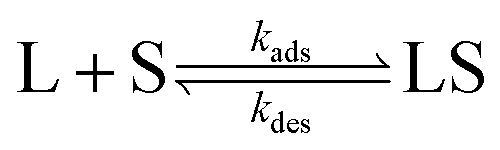
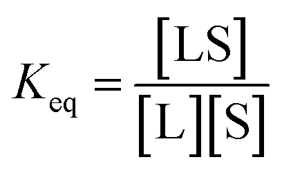 for eqn (1)), for a surface sorption equilibrium in the Langmuir model, the concentration of binding sites is generally unknown and has to be part of the equation. The fraction of surface binding sites occupied by ligands is defined as the surface coverage (θ):