
Optical sensors (optodes) for multiparameter chemical imaging: classification, challenges, and prospects
Andrey V.
Kalinichev
 ,
Silvia E.
Zieger
and
Klaus
Koren
*
,
Silvia E.
Zieger
and
Klaus
Koren
*
Aarhus University Centre for Water Technology, Department of Biology – Microbiology, Ny Munkegade 116, 8000 Aarhus C, Denmark. E-mail: klaus.koren@bio.au.dk
First published on 13th November 2023
Abstract
Chemical gradients and uneven distribution of analytes are common in natural and artificial systems. As a result, the ability to visualize chemical distributions in two or more dimensions has gained significant importance in recent years. This has led to the integration of chemical imaging techniques into all domains of analytical chemistry. In this review, we focus on the use of optical sensors, so-called optodes, to obtain real-time and multidimensional images of two or more parameters simultaneously. It is important to emphasize that multiparameter imaging in this context is not confined solely to multiple chemical parameters (analytes) but also encompasses physical (e.g., temperature or flow) or biological (e.g., metabolic activity) parameters. First, we discuss the technological milestones that have paved the way for chemical imaging using optodes. Later, we delve into various strategies that can be taken to enable multiparameter imaging. The latter spans from developing novel receptors that enable the recognition of multiple parameters to chemometrics and machine learning-based techniques for data analysis. We also explore ongoing trends, challenges, and prospects for future developments in this field. Optode-based multiparameter imaging is a rapidly expanding field that is being fueled by cutting-edge technologies. Chemical imaging possesses the potential to provide novel insights into complex samples, bridging not only across various scientific disciplines but also between research and society.
 Andrey V. Kalinichev, Silvia E. Zieger and Klaus Koren (from left to right) | Andrey V. Kalinichev graduated from St Petersburg State University in 2017. He received his Ph.D. in physical chemistry (2021) from St Petersburg State University. He currently works as a postdoctoral researcher at Aarhus University, Denmark, developing chemical sensors, in particular ionophore-based optical and electrochemical sensors. The scope of his interests also includes computer simulations of the sensor response and the behavior of liquid/liquid interfaces. He has published 15 peer-reviewed scientific articles. Silvia E. Zieger is a postdoctoral researcher who specializes in signal deconvolution and the development of optical chemical sensors. She obtained her Ph.D. in Analytical Chemistry from Graz University of Technology in 2019, under the supervision of Prof. Ingo Klimant. Currently, she works at the Sensor Laboratory and the Center for Water Technology at Aarhus University. Her primary focus is on developing advanced algorithms for multiparametric sensing including signal processing and machine learning modeling approaches. Silvia has published 15 peer-reviewed scientific articles. Klaus Koren obtained his PhD from Graz University of Technology, Austria, under the supervision of Prof. Ingo Klimant in 2012. After working as a postdoc in the laboratory of Prof. Michael Kühl (Copenhagen University, Denmark) he started his independent research group in 2018 at Aarhus University. His research focuses on the development and application of chemical sensors to better understand complex biological systems. Klaus has published more than 60 peer-reviewed scientific articles and received the Fritz-Feigl prize from the Austrian Society of Analytical Chemistry in 2021. |
Introduction
“A picture is worth a thousand words.” It is sayings like this that demonstrate how important visual representations are for us as humans and for that matter scientists. It is much easier to understand if we can see something with our own eyes. Maybe, therefore, chemical imaging has become so popular. Using as diverse methods as mass spectrometry,1,2 Raman spectroscopy,3,4 or X-ray spectroscopy,5,6 scientists have developed approaches to visualize chemical elements or molecules in 2 or even 3 dimensions. While vastly different in terms of the underlying analytical methodology, all those methods can be referred to in one way or the other as chemical imaging. It is beyond the scope of this review to address all these methods, rather this review focuses on chemical imaging using optical sensors, so-called optodes.Contrary to several other chemical imaging methods, optodes often enable the real-time visualization of small molecules (gasses and ions) and often use rather cheap instrumentation. Furthermore, optode-based chemical imaging can also be used to image multiple analytes and parameters at a time. This multiplexing possibility will be at the center of this review. The ambition is to identify and describe different approaches to obtain multiparametric images and to discuss the respective advantages and challenges.
In the field of chemical imaging, it is crucial to establish a clear definition of sensors and their application. There exist various interpretations of the term “chemical sensors”; however, we will focus on two definitions that are relevant to our discussion. The first one is the “Cambridge” definition: “Chemical sensors are miniaturized devices that can deliver real-time and online information on the presence of specific compounds or ions in even complex samples”.7 The second one implies that sensors aim to “obtain information about the substantial matter, especially about the occurrence and amount of constituents including information about their spatial distribution and their temporal changes”.8 Thus, chemical sensors should be designed and utilized in a manner that provides information on the spatial distribution of the analyzed parameter(s), i.e., provides the possibilities for chemical imaging.
Chemical sensors are categorized based on their operating principles, and one of those is based on utilizing optical signals. Optodes convert changes in analyzed parameters (e.g., analyte concentration) into changes in optical phenomena. “Compared to several other imaging techniques, optodes can often be applied in a non-destructive way and respond almost in real-time with typical response times in the range of seconds to minutes and in a reversible fashion. Furthermore, optodes are flexible in their design, allowing chemical imaging over a wide range of scales from single cells (sub-μm) to larger organisms or small ecosystems (dm × dm)”.9
One of the main advantages of optodes is the possibility of multiparameter imaging at the exact same spot and time. In this review, we use the term “multiparameter” as the synonym for “multianalyte”, “multiple”, and “multiplexed”. Conducting chemical imaging with optodes for multiparameter sensing requires addressing various challenges. Those challenges arise as chemical imaging is a highly interdisciplinary field building on developments in fields such as electronic noses/tongues,10 organic synthesis,11 chemometric data processing,12 colorimetric sensor arrays,13 device development,14etc. In this regard, chemical imaging requires bringing all those aspects together and even further utilizing them to address biological or medical questions.
In 2007, Stefan Nagl and Otto S. Wolfbeis claimed the features of true multiparameter sensors:15
(a) Two or more parameters can be sensed at the very same site and simultaneously;
(b) They enable chemical sensors to be compensated for the effects of temperature if combined with a temperature sensor chemistry;
(c) They enable unspecific sensors to be made more specific;
(d) They enable smaller sample volumes to be analyzed for more parameters than with monosensors;
(e) They enable the sensing of several parameters in cases where the sample volume is limited (such as in the case of blood), or in the case of microscopy or microfluidic devices.
For the last 15 years, several comprehensive reviews of imaging with optical sensors and multiparameter analysis have been published (Table 1). This review will focus on the systemization of the present and generally possible approaches to multiparameter chemical imaging with optodes rather than duplicate previously published information.
| Title | Authors | Year | Summary | Ref. |
|---|---|---|---|---|
| Optical multiple chemical sensing: status and current challenges | Stefan Nagl, Otto S. Wolfbeis | 2007 | The first systematic review of true dual optode used for imaging. The authors envisaged introducing triple sensors and sensing schemes for important analytes such as O2, pH, CO2, and temperature | 15 |
| Multiple fluorescent chemical sensing and imaging | Matthias I. J. Stich, Lorenz H. Fischer, Otto S. Wolfbeis | 2009 | A critical review of the state of the art in terms of spectroscopic principles and materials (mainly indicator probes and polymers), and gives selected examples for dual and triple sensors | 16 |
| The art of fluorescence imaging with chemical sensors | Michael Schäferling | 2012 | A review of the basic functional principles of fluorescent probes, the design of sensor materials, and approaches of multiple sensors development and methods for their signal readout | 17 |
| Optical methods for sensing and imaging oxygen: materials, spectroscopies and applications | Xu-dong Wang, Otto S. Wolfbeis | 2014 | A comprehensive review of optical methods for sensing oxygen including spectroscopies and readout schemes in luminescent sensors and multiple sensing techniques | 18 |
| Planar optode: a two-dimensional imaging technique for studying spatial-temporal dynamics of solutes in sediment and soil | Cai Li, Shiming Ding, Liyuan Yang, Qingzhi Zhu, Musong Chen, Daniel C.W. Tsang, Gen Cai, Chang Feng, Yan Wang, Chaosheng Zhang, | 2019 | A comprehensive overview of the research progress on 2D imaging with planar optodes in sediment and soil including the progress in multiparameter imaging | 19 |
| Optical sensing and imaging of pH values: spectroscopies, materials, and applications | Andreas Steinegger, Otto S. Wolfbeis, Sergey M. Borisov | 2020 | The first comprehensive review of methods and materials for use in optical sensing of pH values and on applications of such sensors including commonly used optical sensing schemes, luminescent sensors design, imaging of pH values, and selected applications of these sensors | 20 |
| Optode based chemical imaging—possibilities, challenges, and new avenues in multidimensional optical sensing | Klaus Koren, Silvia E. Zieger | 2021 | A perspective article on novel state-of-the-art technologies for optode-based chemical imaging including the discussion of possibilities for multiparameter imaging | 9 |
| Fiber optic sensor designs and luminescence-based methods for the detection of oxygen and pH measurement | Jan Werner, Mathias Belz, Karl-Friedrich Klein, Tong Sun, K.T.V. Grattan | 2021 | A comprehensive review of luminescence-based fiber optical sensors, sensing methodology, optical sensor platforms, and multiple luminescence sensing concepts | 21 |
Historical overview
To provide robust two-dimensional (2D) imaging, planar optical sensors have been utilized for almost three decades. The first “conventional” imaging setup, which was devoted to O2 determination in benthic communities, was introduced by Glud et al. in 1996.22 However, only one analyte could be measured in 2D at that time. Since then, a lot of progress in this field has been made including approaches to provide simultaneous determination for two or more analytes. Nevertheless, before delving deeper into multiparameter imaging, let us see how it became possible to develop the first imaging setup based on optodes. To do that, we would like to indicate three main sections, the advancement of which made Glud's work possible eventually: Fluorescence and optode development, Sensitive paint utilization and dual sensing, and CCD and CMOS implementation in chemistry (Fig. 1).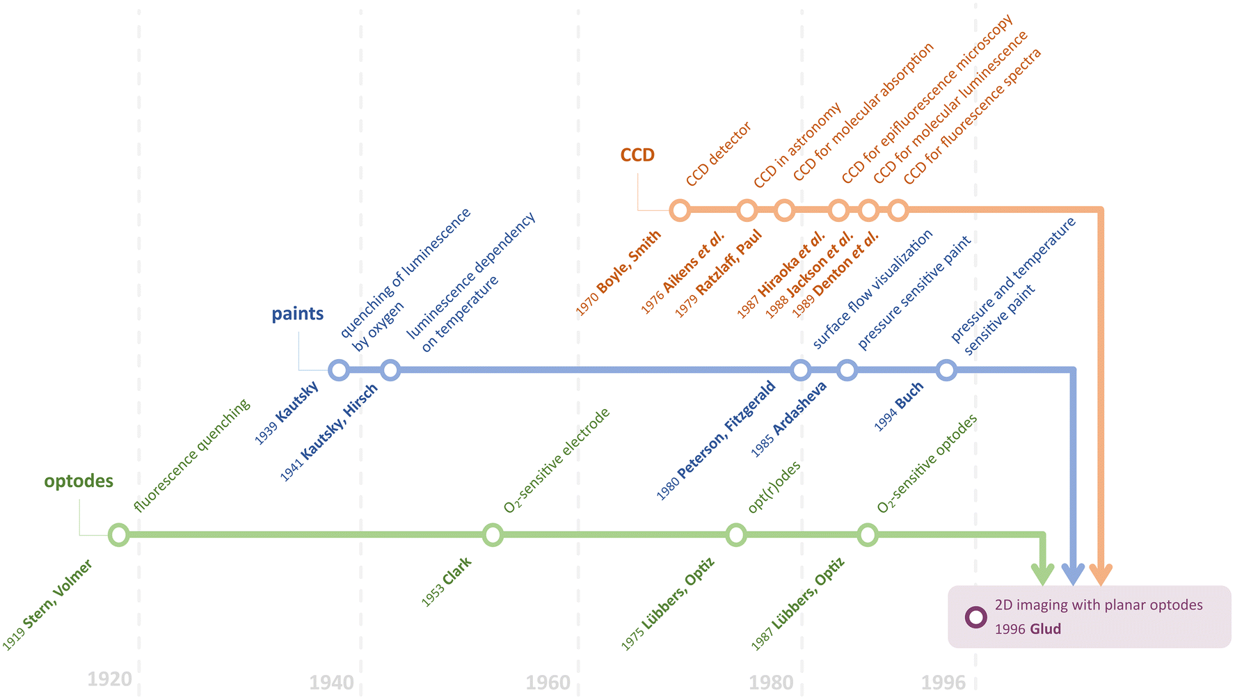 | ||
| Fig. 1 Timeline of milestones in the development of the first imaging setups based on optodes. | ||
Fluorescence and optode development
The journey to optode development might have begun in 1919 when Stern and Volmer published a theory and equation relating the change in fluorescence quantum yield and fluorescence lifetime as a function of added quencher.23 Twenty years later, Kautsky provided reports on the possibility of observing the luminescence quenching effect using oxygen.24 Nowadays, it is generally accepted that almost all the phosphorescence and fluorescence dyes are quenched by molecular oxygen.18,25 Therefore, it is no coincidence that the first implementation of imaging with optodes was devoted to oxygen determination.The term “optode” was introduced by Lübbers and Opitz in 1975.26 By analogy to electrodes, they called such an optical sensor with an indicator film separated by a membrane from the sample an optode. The latter is a reason optodes might still be called opt(r)odes since it is a combination of two words “optical” and “electrode”. They began the investigation of optical measurement of gas pressures (especially oxygen) using fluorescent dyes. It appeared to be a bifurcation point in the era of dissolved and gaseous oxygen measurements predominately done using Clark electrodes27 since the O2 optode did not consume oxygen and a reference electrode was not required anymore. In 1987, Opitz and Lübbers published a comprehensive overview of the theory and development of fluorescence-based optochemical oxygen sensors.28 In this article, they demonstrated the superiority and perspective of using optodes in general.
Sensitive paint utilization and dual sensing
The first sensor most similar to 2D optodes was sensitive paint.29 Pressure-sensitive paints (PSPs) have been developed for measuring air pressure on surfaces. The response mechanism of PSPs is also based on luminescence quenching by molecular oxygen, which was established by Kautsky. Peterson and Fitzgerald demonstrated a preliminary approach for surface flow visualization using spray-coating on shapes of interest in 1980.30 This approach led to the development of PSPs in 1985 by Ardasheva et al.31 Since that time, it has become possible to determine at least one of the quantitative parameters in 2D. However, this emerging field of chemical imaging unintentionally unlocked the possibility of performing simultaneous dual measurements.In 1931, Kautsky and Hirsch obtained luminescence dependency on temperature.32 Although the basis of using luminescence probes for dual sensing had been known for many years, one of the first reports was published only in the 1990s. Buck suggested using perylene dye sorbed on silica to perform simultaneous luminescence pressure and temperature measurements using paints.33 Despite the possibility of dual sensing with optical sensors, the temperature cross-sensitivity was a significant interfering factor for numerous real applications. Thus, researchers tried not to utilize this feature of the luminescent dyes but to eliminate it. Coyle and Gouterman proposed a method of correcting lifetime measurements for temperature by adding a non-oxygen quenched, temperature-dependent phosphor.34
CCD and CMOS implementation in chemistry
Unarguably, modern chemical imaging is not possible without digital imaging devices. Widely used devices such as monochrome, color, hyperspectral cameras, or scanners are based on the three main sensor types and device architectures, namely, CCDs (charge-coupled devices), CMOS (complementary metal–oxide-semiconductor) and CIS (contact image sensor). To trace the path that led Glud et al. to utilize the CCD camera, let us turn to the beginning.Boyle and Smith developed the concept of a charge-coupled detector in 1969.35,36 The scientific applications of CCDs were first demonstrated in astronomy research in 1976.37 However, a chemical application was first demonstrated by the CCDs’ utility in a spectroscopic measurement; Ratzlaff and Paul employed a linear CCD for molecular absorption in 1979.38 They showed that the CCD-produced signals are linear with both intensity and integration time in the visible region. For the proof-the-concept, the absorbance spectrum of the calibration tool, the didymium oxide filter, was recorded within 250–750 nm. Subsequently, the high sensitivity of CCDs made these devices well-suited to molecular luminescence measurements. The properties of CCDs and their application to the high-resolution analysis of biological structures by optical microscopy were shown for three-dimensional imaging using an epifluorescence microscope in 1987.39 In 1988, the first 2D visualization of fluorescently labeled objects was reported by Jackson et al.40 Furthermore, Denton et al. demonstrated the acquisition of fluorescence spectra for the first time in 1989.41
Although it is Glud's optode design (Fig. 2B) that one could consider as “conventional” now, the combination of CCD camera and optical sensor fibers was reported by Bronk et al. a year earlier, in 1995.42 The authors used approx. 6000 optical fiber-sensors in a bundle with a 4 μm spatial resolution (Fig. 2A).
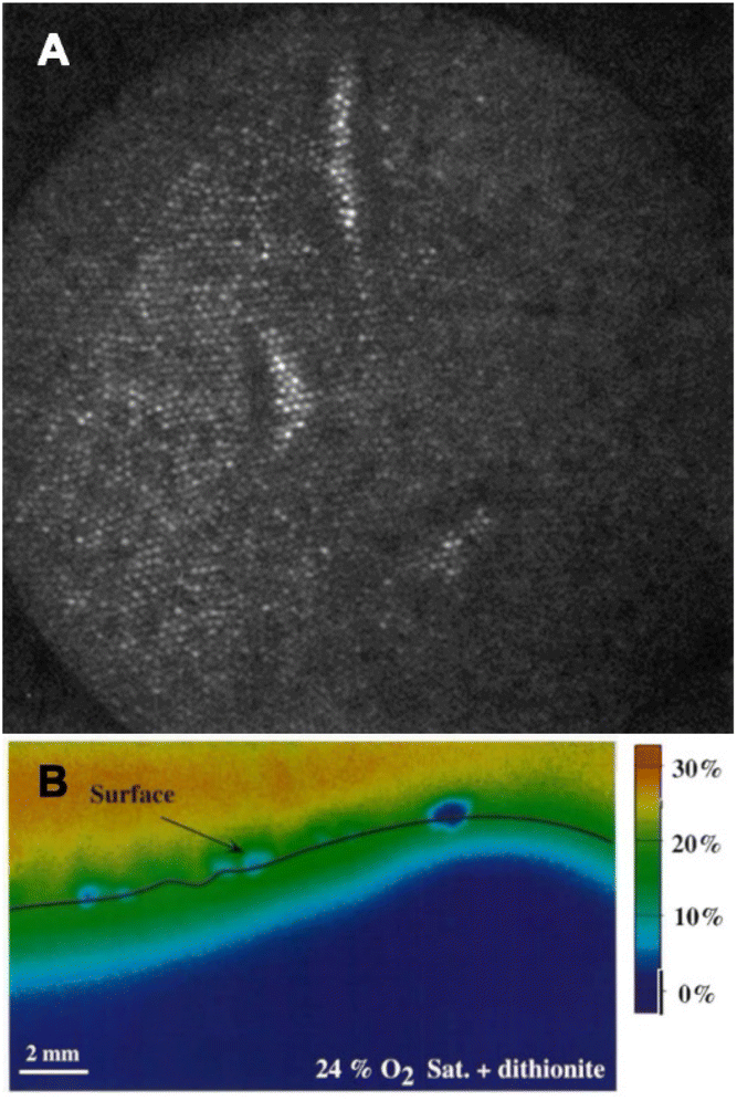 | ||
| Fig. 2 Different designs of multiparameter optodes. (A) Fiber-bundle sensor design: polyHema/fluorescein-modified imaging fiber with mouse fibroblast cells.42 (B) Planar 2D sensor design (“Glud's design”): calibrated images of the O2 distribution at the sediment-water interface with sodium dithionite grains added.22 Reprinted with permission from ref. 42. Copyright 1995 American Chemical Society. | ||
Nowadays, although CCD image sensors are still used in some high-end cameras and scientific applications, CMOS sensors, invented in 1963 by Wanlass and Sah,43 have emerged as the predominant technology in consumer electronics. This transition has primarily occurred due to the cost-effectiveness, energy efficiency, and rapid processing capabilities offered by CMOS sensors.
The road to multiparameter sensors
Thus, both improving knowledge of physicochemical processes and technological advancements played pivotal roles in devising strategies for chemical imaging. Nearly three decades have passed since 1996. Consequently, what are the most significant changes that have occurred during this period? It is challenging to precisely identify these changes; however, we would like to highlight some we consider essential, namely: (1) advancing chemical materials and utilizing different modes of signal formation/readout, (2) using different approaches to create optodes including nanoparticle formation, (3) utilizing technologies beyond monochrome CCDs including color and hyperspectral devices. Eventually, the combination of these factors has led to a push towards multiparameter imaging.Undoubtedly, the latter is paramount to gaining a more comprehensive understanding of the analyzed system, especially where the distribution of the analytes measured simultaneously might reveal any intimate interplays between them. For instance, the dual determination of oxygen and carbon dioxide at the same time and in the same spot could shed light on oxidative respiration and photosynthesis process differentiation. This problem was in fact tackled by the first created dual imaging setup based on optodes.44
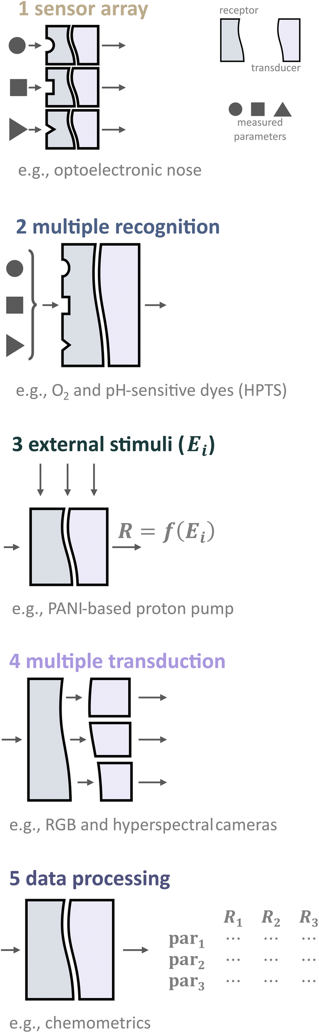
Before diving into examples, we must ask, how can one create a multiparameter optical sensor in general? To address this question, let us look closer at what an optode is as well as what components and steps are involved to obtain physicochemical information from samples (Fig. 3).
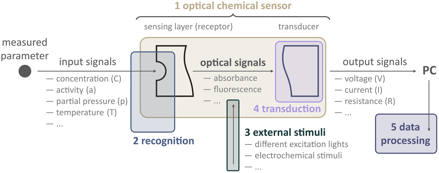 | ||
| Fig. 3 Schematic depiction of measurements conducted using optical chemical sensors. The color blocks and numerical annotations indicate the specific sites enabling the simultaneous analysis of multiple parameters, presented in the order listed (see text for more details). PC denotes the personal computer. | ||
Optodes are optical sensors that translate information about samples into optical analytical signals. The type of information could be different: from physical (temperature, partial pressure) to chemical (analyte concentration or activity). We would like to underline that an optode should be considered not as a probe or sensing film per se but rather as a compound device. Conventionally, an optode includes two parts: a sensing element (receptor) and a transduction element (transducer). The receptor provides the recognition of a parameter being analyzed, e.g., the concentration of a measuring analyte, temperature, pH, gas partial pressure, etc. Providing that the optode changes at least one of the optical properties (absorption, fluorescence, reflectance, refractive index, optical activity, surface plasmon resonance, etc.) depending on the magnitude of the parameter. The transducer converts the optical signal generated by the receptor (the actual concentration value, a non-electric quantity) into a measurable signal that is appropriate for processing, i.e., an electric quantity: voltage, current, or resistance.8
Consider, for instance, the first 2D imaging setup described by Glud et al.22 In this case, the sample was a marine sediment, and the authors were interested in measuring O2 concentration over both space and time. To achieve this, they prepared an O2-sensitive luminescent optode. The receptor of this optode kind consists in its most primitive form of an oxygen-sensitive dye (indicator) dispersed within a host polymer, which is applied onto a transparent surface, such as a glass plate or polymer foil.
In addition to those basic components, others can be added, like enhancers (scatters like titanium dioxide or diamond particles) and additional dyes (for referencing). Furthermore, this optode layer might be protected by an optical isolation layer, which serves to minimize the influence of ambient light on the sensor while not interfering with the chemical receptor.
When this optode comes into contact with the sample, excitation light is needed to excite the luminescence of the dye, and a detector (e.g., camera) to record the emission of the receptor. Filters are employed to ensure that only the analytically relevant light reaches the camera. In summary, a basic chemical imaging starter kit needs some sensor chemistry, including indicators and a host polymer, a light source, filters, and a camera. Remarkably, this is the very same configuration that Glud and co-workers used in their pioneering work, and it continues to be employed today in similar research.
In addition to this conventional setup, in recent years, researchers have explored the use of external stimuli to enhance data collection from sensors. In this context, an external stimulus refers to any external changes or influences that can impact the response of a sensor. For instance, the luminescence of a sensor can be affected by temperature changes. Therefore, altering the temperature during analysis can lead to variations in the sensor response. Additionally, when using a luminescence-based optode, it is necessary to use excitation light to trigger the sensor. Let us assume that an optical sensor consists of several indicators. Changing the excitation wavelength, in this case, results in altering the emission spectra of the optical sensor. Consequently, applying external stimuli causes the measurement signal to depend not only on the parameters being analyzed but also on the nature of the stimulus itself. By considering these factors, the use of external stimuli opens possibilities for distinguishing between different analytes or their compositions. This, in turn, facilitates multiparameter analysis.
Thus, to enable simultaneous analysis of multiple parameters, various approaches can be classified based on the processes or designs involved, as shown in Fig. 4. These approaches include (1) sensor arrays, (2) dual/multiple recognition, (3) changing external stimulus, (4) multiple transduction, and (5) utilizing chemometric techniques.
 | ||
| Fig. 4 Designs of optical sensors and involved processes provide multiparameter analysis. | ||
Multispot sensors and sensor arrays
Multispot sensors and arrays are composed of single sensor systems for given analytes, merged and miniaturized to a compact optical sensing device.16 Nowadays, the most common approaches to making sensor arrays are using optical fibers (fiber bundles)21 and the microspheres of optical sensors in microwells.45 Recently, a similar technique to the last one has been widely utilized in tissue profiling approaches.46 The recent comprehensive review on the development and state-of-the-art of colorimetric and fluorometric sensor arrays has been published in 2019.13Although this approach for simultaneous measuring several parameters is cost-efficient and relatively easy, sensor arrays do not fulfill the requirement of determination of analyzed parameters in the same compartment. Usually, the distance between the adjacent elements is 5–20 μm; however, depending on the array geometry, measurements can be up to several 100 μm apart. This can be considered a large distance, in particular in systems where steep chemical gradients form like within biofilms.47
Recognition
As mentioned, recognition is the first step to obtaining sensor response. Typically for planar optodes, the receptor function is fulfilled by a thin layer that can interact with analyte molecules or participate in a chemical equilibrium together with the analyte.8 For example, the most important processes underlying the response of ion-selective optodes are ion exchange and co-extraction in the case of cation- and anion-selective optodes, respectively.48One of the key properties of the recognition phase of optode response is selectivity. Selectivity is the ability of the sensor to respond preferentially to the analyte but not to an interfering species or interfering parameter. However, there is no one absolutely selective sensor, and some cross-sensitivities are generally always present. Should one acknowledge such cross-sensitivities as a possible source for multiparameter analysis? We think—yes—if any approaches allow the determination of both the analyzed and the interfering parameters separately.
Luminescence intensity. In luminescent sensors, the excitation of an indicator dye leads to the emission of photons either via fluorescence or phosphorescence. Those photons generally have a lower energy (longer wavelength) than the excitation light and the amount of those photons (intensity) can be correlated to an analyte of interest. Take for example the classical optical oxygen sensor. Paramagnetic O2 is an effective luminescence quencher resulting in reduced indicator emissions with increasing oxygen concentrations.18 In this way the intensity of the indicator emission can be correlated to the O2 concentration following e.g., the Stern–Volmer relation.
Despite this being a very straightforward approach relying solely on luminescence intensity can be problematic as also other factors than the analyte concentration can influence this parameter. Those factors include fluctuations in the excitation light, bleaching of the indicator, or simply uneven distribution of the indicator within the sensor.49 Currently, these limitations are often overcome by adding a second, inert, dye into the sensor matrix.50,51 In this way the emission of the two dyes can be set into proportion (ratio) enabling a more robust readout as several of the factors mentioned above can be eliminated or reduced. At the same time, the use of an extra reference dye comes with challenges in terms of multiparameter imaging. Separating the reference signal from the indicator signal is one of those.
Luminescence decay time. Contrary to the above, decay time-based imaging does not use the amount of photons to quantify an analyte, but rather another property of the emitted photons, their decay time. The decay time represents the average duration between photon excitation and emission and can range from nanoseconds to milliseconds, depending on the indicator and the type of luminescence used (e.g., phosphorescence or fluorescence). Measuring decay time offers several advantages over intensity-based methods. Firstly, the decay time is not affected by the concentration of the indicator. No additional referencing (additional dye) is needed as decay times as such is intrinsically referenced. Additionally, fluctuations in the optical setup have less impact on the measurement.49
On the flip side, chemical imaging based on decay times requires somewhat more sophisticated equipment. Essentially, cameras used for this approach need to be able to measure (time) when photons are emitted relative to the excitation, either in the time or frequency domain. In a recent article, we evaluated those approaches, and the interested reader is referred to this study.52 While being technically more challenging, decay time-based imaging enables the separation of multiple signals not only on spectral but also temporal domain. This capability holds significant potential for applications in multiparameter imaging.53
Combination of luminescence and decay time. It is also possible to combine different detection schemes. For instance, HPTS (8-hydroxypyrene-1,3,6-trisulfonic acid) was used to measure both pH and O2.54 In order to measure pH and the concentration of oxygen, various optical properties were measured. Specifically, pH was determined by analyzing the ratio of intensities between the isosbestic point and the emission peak of the HPTS anion. Meanwhile, oxygen concentrations were measured based on fluorescence decay time, which decreased as the oxygen concentration increased.
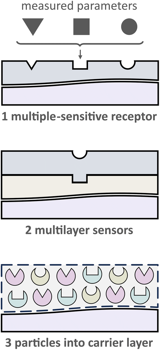 | ||
| Fig. 5 Schematic of the three most common designs for creating multiparameter optical sensors via different recognition options: (1) multiple-sensitive receptor, (2) multilayer sensors, (3) (nano)particles into carrier layer. | ||
2.2.1. Receptors that are sensitive to several parameters. One evident and desirable solution for multiparameter sensing is using chemicals that are sensitive toward at least two parameters each with a distinct influence on the optical properties, either spectral or via decay time (Fig. 5). It is generally challenging to find a suitable dye or pigment to measure two or more parameters simultaneously. However, one can argue that one natural additional parameter for measuring is temperature as it affects every sensor. Nevertheless, the latter enables temperature compensation which could be essential to reduce measurement errors.
Typically, the fluorescence intensity or fluorescence decay time of a single luminophore is used for multiparameter sensing. In section 2.1.3, HPTS is shown as an example of a probe selective to O2 and pH simultaneously. Other indicators for the determination of two parameters (pH/O2, pH/T, O2/T,56 CO2/O2, pH/Cl−) were proposed. More details can be found in section 10.7 of ref. 20.
Nevertheless, other types of luminescence are also used to achieve multiparameter sensing. Schwendt and Borisov showed that the simultaneous monitoring of O2 and temperature can be achieved with a single metalloporphyrin-based indicator through thermally activated delayed fluorescence (TADF) and phosphorescence.57 O2/T determination was demonstrated for a naphthoquinone-extended Pt(II) benzoporphyrin embedded in polystyrene, which operated within temperature region from 5 to 55 °C and oxygen partial pressure from 0 to 202 hPa.
Recently, diazobenzocrowns with pyrrole residue as a part of the macrocycle were utilized as a dual Pb2+/pH indicator.58 The authors suggested using absorption followed by digital color analysis. Both pH and lead(II) concentration influence optical signal: increasing lead(II) concentration leads to the color change from pink to blue-gray.
In addition, there are functional synthetic probes for multiparameter sensing.11 Although it is possible to distinguish three main aminothiols (homocysteine, cysteine, glutathione) due to producing three distinct products and fluorescent emission signals in blue, green, and yellow channels, it was demonstrated for imaging in live cells only.59 Thus, there is enough room for collaboration with organic synthesists and for implementing such probes for planar 2D imaging of similar analytes.
2.2.2. “Sandwich” sensors. The scarcity of existing probes for multiparameter sensing via a single dye can be overcome by utilizing multilayer sensors (Fig. 5). This kind of sensor is based on the use of two or more layers, each of which contains single-selective receptors. Besides that, different analytical signals from each layer could be utilized to differentiate various parameters. Nevertheless, even though “sandwich” sensors allow to performing true multiparameter sensing at identical sites, there are some drawbacks. Stefan Nagl and Otto S. Wolfbeis revealed these disadvantages as follows:15 (1) cross-sensitivities concerning the analyte as well as spectral crosstalk including FRET and PET processes, (2) cross-leaching of the components between layers, and (3) increased photodecomposition and signal drift compared to single sensors.
Despite all the drawbacks, the rather easy fabrication of such multilayer sensors and the increasing popularity of cameras with >3 color channels are the main reasons for the increased use of this sensor type.60
2.2.3. Polymer binder with (nano)particles suspension. An effective solution to address the challenges described above involves compartmentalizing the sensing chemistry for specific applications. This can be achieved by preparing nano- or micro-particles that are sensitive to a specific analyte.61,62 In this way, each particle can be designed to provide a favorable microenvironment for the respective sensor chemistry. These multiple particle-based sensors can then be combined into a single layer (see Fig. 6). To hold these particles together, a suitable binding material, or “binder”, is needed.
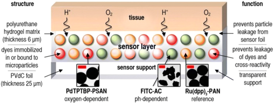 | ||
| Fig. 6 Scheme of multiparameter (pH, O2, and T) optical sensor with (nano)particles suspension.63 Oxygen-dependent palladium(II)-meso-tetraphenyltetrabenzoporphyrin incorporated in oxygen-permeable poly(styrene-co-acrylonitrile) particles (Pd-TPTBP-PSAN), pH-sensitive fluorescein-isothiocyanate bound to aminocellulose particles (FITC-AC), and the pH-independent reference dye ruthenium(II)-tris(4,7-diphenyl-1,10-phenanthroline) in oxygen-impermeable polyacrylonitrile particles (Ru(dpp)3-PAN). Microparticles were embedded in a polyurethane hydrogel matrix on poly(vinylidene-chloride) (PVdC) foils. Dye leakage was prevented by binding the dyes to or incorporating them into microparticles. By embedding the particles in the hydrogel, leakage of particles from the sensor was also prevented. The insets show transmission electron-microscopic (TEM) pictures of the sensor particles (bars: left and right image 0.5 μm, middle image 2 μm). | ||
Hydrogels are particularly suitable for this purpose due to their biocompatibility and hydrophilic nature, which helps prevent the often hydrophobic components of the particles from leaching into the surrounding matrix.15 This approach has enabled the development of multiparameter imaging techniques for various applications. For instance, the collaboration between the research group led by Wolfbeis and medical professionals has demonstrated how extracellular pH gradients and tissue hypoxia affect wound healing in chronic wounds.63 Those insights have been made possible by using a dual O2/pH optode employing three types of particles within the same matrix (Fig. 6).
Importantly, this innovative approach is not limited to medical applications, as shown by Fischer et al.64 In this study, a technique involving spray painting was utilized to color complex structures with a mixture of O2 and temperature-sensitive particles. This novel pressure-sensitive paint method offers the advantage of easy application through spray painting and straightforward removal by washing the coating off with water. The proposed approach is more environmentally friendly while still providing high-resolution images for monitoring of O2 and T.
External stimuli
External stimuli could be used to alter the response signal of the sensor. For example, the analytical signal might be dependent on a stimulus such as temperature, pressure, pH, humidity, or light. One could implement this dependency deliberately by incorporating specific materials or components into the optode matrix that are sensitive to these external stimuli. These components can then trigger a change in the optical properties of the sensor, resulting in a measurable change in the response signal. However, conventionally used dyes and other active components could also be sensitive to changes in temperature, pH, humidity, etc.Moreover, the use of external stimuli can provide a way to control and manipulate the sensing properties of optical sensors, creating more versatile platforms for multiparameter imaging. By tuning the external parameters, the response signal or readout of the sensor can be controlled, providing the ability to discriminate different parameters or to enhance the sensitivity and selectivity of the sensor.
Unfortunately, this approach is concerned with the destruction of the sample being analyzed. Furthermore, in samples containing intricate matrices, such as blood, the introduced chemicals may easily alter the properties of the sample itself, thus resulting in the infeasibility of analysis or significant inaccuracies in the interpretation of the results.
Borisov et al. introduced the first quadruple luminescent sensor for measuring O2, CO2, pH, and temperature.66 The multilayer sensor combined two spectrally independent dually sensing systems; the latter was possible due to the use of color filters and two different excitation lights: a blue LED (450 nm) for CO2/O2 and a red LED (605 nm) for pH/temperature sensitive layer. The schemes of the sensor and measuring setup are shown in Fig. 7.
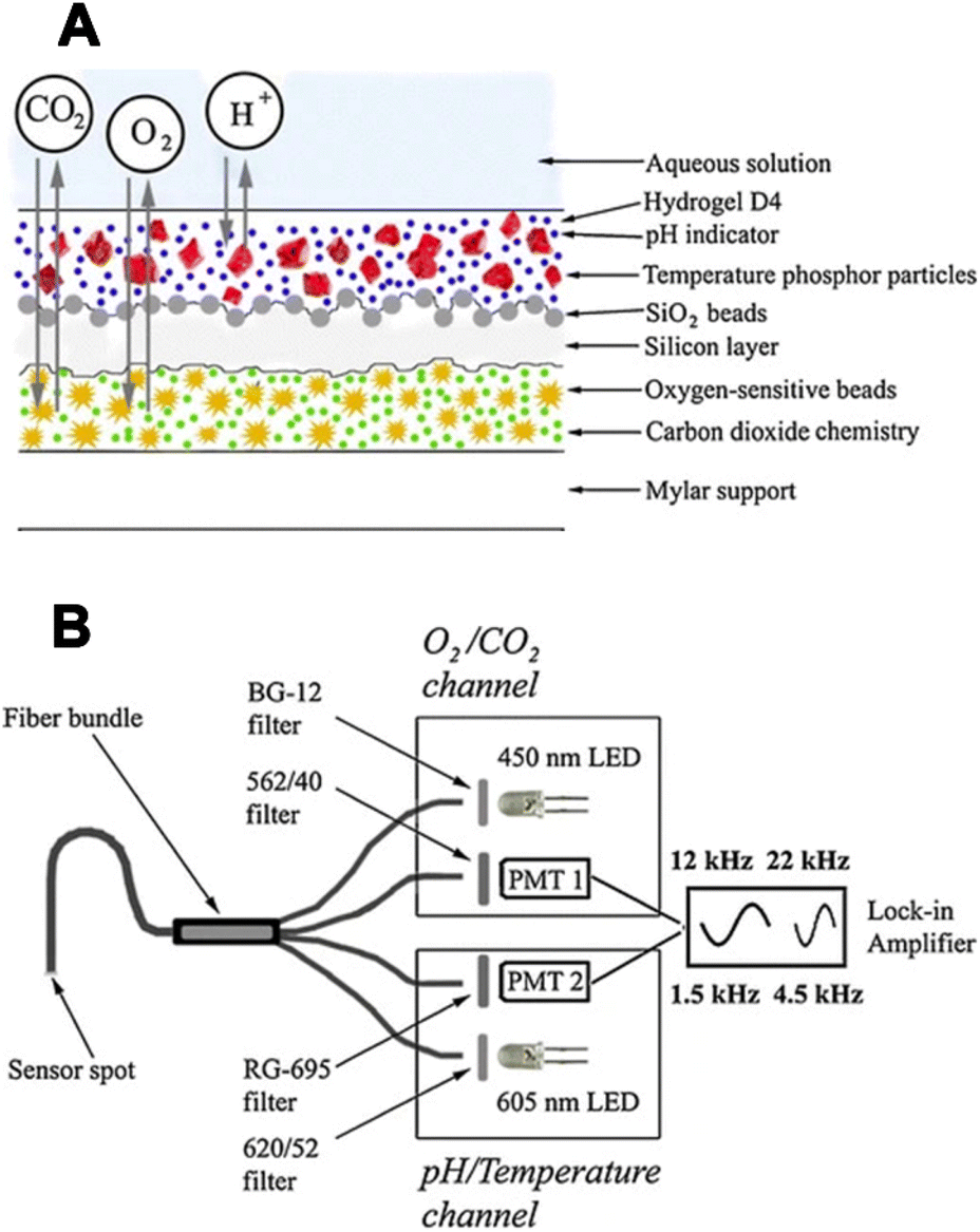 | ||
| Fig. 7 The first quadruple luminescent sensor for measuring O2, CO2, pH, and temperature.66 (A) Cross-section of the multi-analyte sensor. (B) Schematic representation of the device and the optical arrangement for interrogation of the multi-analyte sensor. The device consists of dual detection channels, each equipped with an LED and a photomultiplier module (PMT). Excitation is achieved with LEDs and appropriate filters, and emission light is filtered accordingly. LED modulation was carried out using a two-phase lock-in amplifier at distinct frequencies for each channel. | ||
In a follow-up study, Wiorek et al. combined the same 2D proton pump with a CO2 optode, enabling the imaging of dissolved CO2 and subsequently total dissolved inorganic carbon (DIC).69 Based on those two images, total alkalinity, and pH images can also be calculated based on certain assumptions. Thus, this setup represents a four-parameter imaging approach (Fig. 8). However, it should be noted that the acquisition of the two images (CO2 and DIC) involves a time delay of approximately 10 minutes, which violates the definition of a sensor should sense both parameters simultaneously at the same point. This limitation should be considered, particularly in fast-changing systems, although it is less problematic for systems in a steady state.
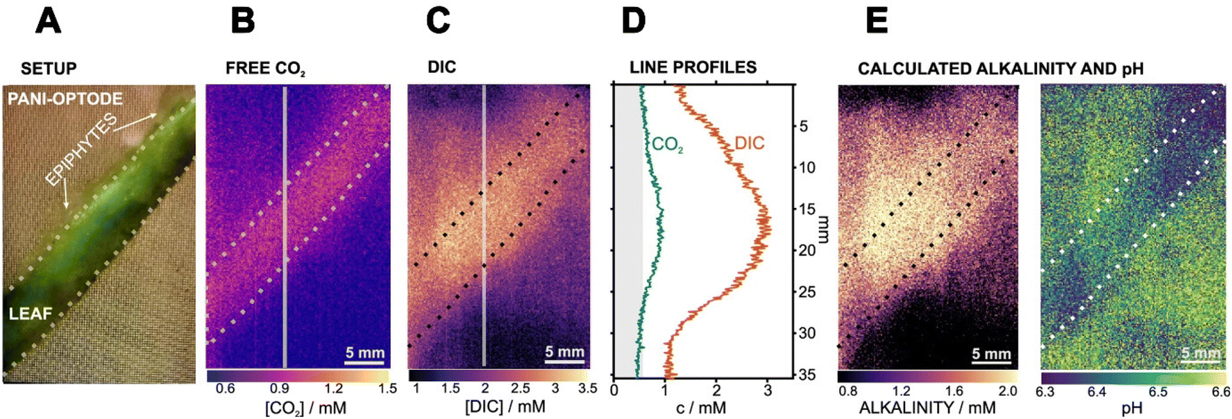 | ||
| Fig. 8 Imaging of an epiphyte-covered leaf of the freshwater plant V. spiralis during dark respiration with PANI-based CO2 and DIC optode.69 (A) Setup of the leaf on top of the PANI-optode architecture. (B) Image of free CO2 after 1 h of incubation in freshwater under dark conditions. (C) Image of DIC right after PANI-based acidification. (D) Line profiles for CO2 and DIC are associated with the gray lines traced in (B and C) from the top to the bottom area. The gray area represents values below the CO2 optode calibration range. (E) Calculated images for carbonate alkalinity and pH. | ||
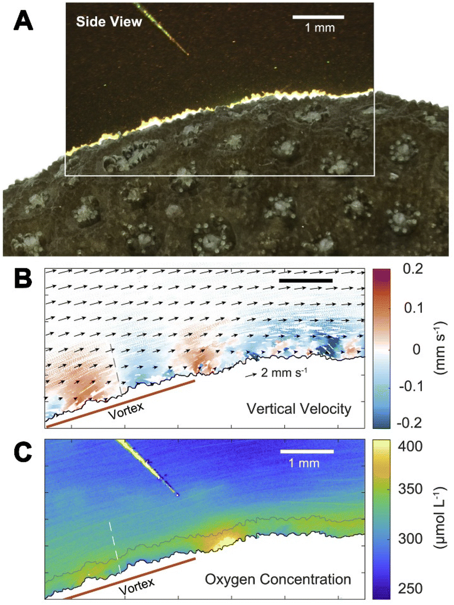 | ||
| Fig. 9 The flow and O2 visualization around corals with the sensPIV approach.70 (A) Color image of sensPIV particles around the coral surface (in the top left corner, the O2 microsensor used to cross-reference measurements). (B) Combined particle image velocimetry (PIV) and particle tracking velocimetry graph of sensPIV particles. Arrows indicate the flow along the coral's surface. Colored dots represent individual particles, and the color indicates the velocity component perpendicular to the coral. (C) 2D mapping of O2 concentration inside the coral boundary layer obtained with sensPIV. | ||
This example highlights that multiparameter imaging is not only limited to multiple chemical species but also includes physical parameters. Furthermore, it shows how entwined processes are in nature and how important multiparameter sensing is to be able to untangle these intricate processes.
Multiple transduction
Generating an optical signal through the recognition stage alone is insufficient for conducting analysis using optical sensors. The next crucial step for quantitative analysis using any analysis tool, in addition to the naked eye, is the transduction stage. As mentioned, conventional devices for chemical imaging coupled with optodes are digital cameras. In this case, metal–oxide semiconductors function as transducers. Here, we want to look at multiple transducers for intensity-based imaging with optodes.Let us imagine using an RGB camera to measure two parameters independently with color referencing. For that, one needs to use a system based on three dyes: a reference dye, a dye selective to the first parameter, and a dye selective to the second parameter. To minimize the possible errors and uncertainties, each dye must emit light only in R, G, or B channels. It leads to two significant disadvantages: (1) spectral properties of the indicators must match an absorption spectrum of color filters and (2) chosen dyes must have a negligible spectral overlap with each other. Thus, to measure more than two parameters with this approach is almost impossible with RGB digital cameras.
Modern cameras with a dual RGB/NIR (near-infrared) chip might help to overcome the spectral overlapping of several luminophores. Moßhammer et al. showed that utilizing RGB/NIR camera provided a dual-analyte for imaging setup optimized to have low cross-sensitivity between the two analytes O2 and pH.51 OHButoxy-aza-BODIPY was the chosen pH indicator that had emission in the NIR channel, while Eu(HPhN)3dpp was used as an O2-sensitive dye with a narrow emission fitting the red channel.
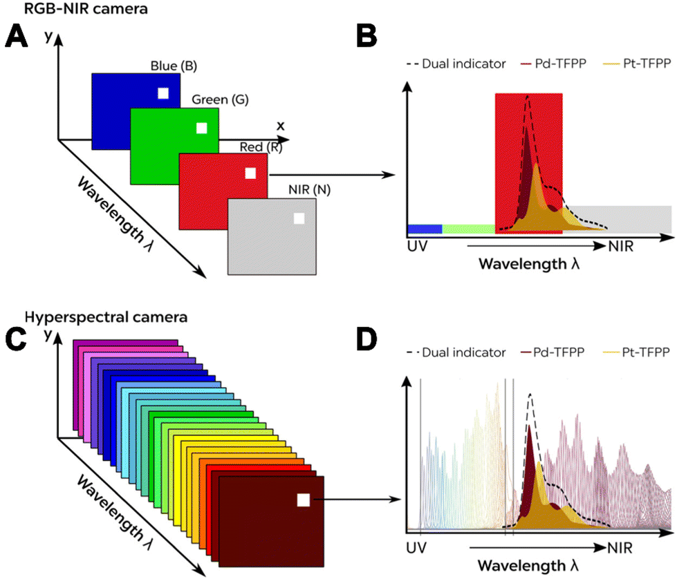 | ||
| Fig. 10 Comparison of (A) a 4-channel RGB-NIR system with (C) a 150+ band hyperspectral camera system. (B and D) Respective information obtained for the emission spectrum from individual and combined optical O2 sensors.72 Reprinted with permission from ref. 72. Copyright 2021 American Chemical Society. | ||
For instance, Kühl et al. utilized an advanced hyperspectral visible near-infrared (NIR) camera system for imaging O2 levels and metabolic activity (respiration and photosynthesis) in a single sample.73 This approach demonstrated that optodes not only enable imaging of physicochemical parameters but also extend to biological measurements. By employing techniques like hyperspectral imaging, microscopy, and O2 imaging, this study revealed that Chl f-containing cyanobacteria in beachrock biofilms exhibit significant NIR-driven oxygenic photosynthesis, particularly crucial for primary production in shaded environments. Such studies provide promising tools for unraveling the ecological importance of intricate interactions within real-world complex samples.
Hence, from a technical point of view, HSIS approaches pave the way for more promising concepts of intensity-based multianalyte imaging with two or even more analytes. However, the sole use of such HSIS does not grant multiparameter imaging per se. To make this ultimately possible, image and signal processing, including chemometric techniques, must be employed. The problem of accessing multiparameter imaging can thus be compared to the task of performing multivariate calibration based on spectral data. In this context, we have already shown that depending on the strength of the optical overlap of the different receptors, signal deconvolution can be achieved either with simpler algorithms such as spectral linear combination and least-square fitting72 or with more complex machine learning algorithms.74
Chemometric analysis
According to the order-based classification of sensors,75,76 single-selective planar optical sensors are at least four-order sensors, given that their output signal (R) is dependent upon four variables: the magnitude of the analyzed parameter (C), chosen wavelength (λ), and the position in 2D (x and y):| R = f(C, λ, x, y). |
In the case of multiparameter imaging, the amount of data in the output signal becomes enormous. Not only that the number of variables change from an individual analyzed parameter (C) to a list of i different parameter values, denoted as C = {C1, C2, …, Ci}, but the number of wavelengths j at which the total signal response of the optode is acquired, denoted as λ = {λ1, λ2, …, λj}, also increases. In addition, the sensor can be subjected to k different external stimuli (E), denoted as E = {E1, E2, …, Ek}.
Considering the temporal variation (t) being a part of the sensor response as a spatiotemporal variable (P), denoted as P = {x, y, t}, the sensor response is a point in the high i × j × k × 3 multidimensional space:
| R = f(C, λ, E, P). |
To address the challenge of translating this large amount of data into valuable information and to enable multiparameter analysis, diverse chemometric techniques must be applied. Thus, chemometrics as a multivariate approach to assessing overlaid signal responses is an essential tool in imaging with optode sensors and has become increasingly important over the years.77 It involves extracting chemical information from datasets generated by imaging sensors to identify patterns and relationships between the measured parameters. The most pivotal aim, where chemometrics is employed, is developing multivariate calibration models, which are used to predict the characteristics of unknown samples.12 However, it should be noted that a significant limitation of chemometrics is the need for extensive experimental characterization and data treatment.
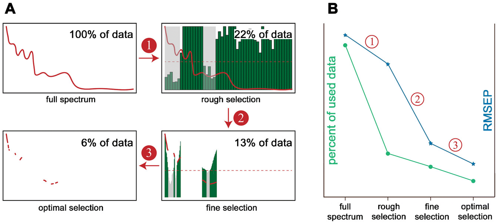 | ||
| Fig. 11 Different feature extraction strategies.81 (A) Flow chart with 3 steps using NIR hyperspectral images of tobacco. Step 1: rough selection, wavelength interval selection method is used to select several intervals with low prediction errors. Step 2: fine selection, make further selection by the methods that can produce a sort of variable based on a criterion and eliminate the variables not satisfying a defined threshold value (red dashed line). Step 3: optimal selection, optimization algorithms are used to search for an optimal variable combination from the variables remained by the steps of rough selection and fine selection. (B) The trend of the percent of data used (number of variables) and root mean square error of prediction (RMSEP) from full spectrum to optimal selection. | ||
Upon selecting the discriminative features, one can either use the specific spectral bands as such or combine these spectral bands to create a new combined feature parameter in a sub-space independent from the original feature space.83 When selecting certain features from the entire data set, different approaches are available depending on the given data set and the intended analysis (features dependency, quantity of available features, and general data quality). Torrione et al.80 summarized the main approaches for feature extraction relevant to spectroscopic techniques. They classified approaches ranging from feature extraction based on expert knowledge and visible inspection of spectral peculiarities in each data set84 to automatic and independent feature search, using, among others, discriminant analysis approaches or sequential search techniques, to multivariate statistical dimension reduction, such as principal component analysis (PCA)83 or partial-least-square (PLS).80 In addition to these approaches, with the forthcoming of machine learning approaches over the past decade more and more approaches are presented using machine learning models for automated (but sometimes indirect) feature extraction. Two examples that should be mentioned here are the random forest algorithm for feature selection85 and the autoencoder.86 While the first algorithm is a machine learning approach combining an ensemble of independent decision trees, the latter one is an approach that aims to reconstruct its input data while performing dimensionality reduction and extracting relevant features.86,87 However, since the field is constantly expanding and this is beyond the scope of this review, the interested reader is referred to respective reviews.88
In this context, multivariate calibration means that rather than focusing on and calibrating for a single target analyte, or more broadly parameter, multivariate models aim to calibrate multiple parameters that affect the response of the sensor.12 Thereby, more information can be obtained about the sample than if each variable were considered separately. This is what Paul Gemperline calls the multivariate advantage.95 However, this multivariate approach requires more information by collecting more sample parameters, as well as more process steps, including signal separation and classification.96 Historically, multivariate calibration has been used only for spectroscopic data such as absorbance and fluorescence emission, but it is not limited to this, and one could include other sample parameters if relevant to the problem at hand.97 In addition, while multivariate calibration was previously omitted by chemometricians, it has become a very popular field in recent years.93 Early algorithms in multivariate calibration still assume linear contributions of different compounds in complex mixtures, and most approaches use principal component regression (PCR), partial least squares (PLS), or so-called multiway or multimode algorithms, with PLS being the most popular.95,98,99
However, with the continuous improvement of mathematical algorithms and signal processing opportunities, chemometricians are striving to incorporate novel algorithms that allow them to analyze increasingly complex situations and to account for non-linear contributions of different compounds in complex mixtures.79 Sometimes it might already be sufficient to extend the aforementioned approaches into a higher dimension, thus enabling a multi-way analysis for example in parallel factor analysis (so-called PARAFAC).100 PARAFAC is a generalization of PCR that requires lightly more complex methodological procedural steps to extract component information from mixed 3D fluorescence data.101 However, for PARAFAC to be useful, certain requirements must be met, such as variability of analyte contributions (no identical spectra), trilinearity of sample parameters, e.g., emission spectra are invariant across emission wavelengths, and increase linearly with the concentration and intensity, and that the overall signal is due to the linear superposition of a fixed number of components.100 Other common expansions to deal with trilinearity besides PARAFAC include the Tucker model and multi-way partial least squares regression.102 Although these algorithms provide great potential, some complex non-linear systems can only be solved by inherently non-linear machine learning algorithms, including naïve Bayes regression, k-nearest neighbor (KNN), support vector machine (SVM), or artificial neural network (ANN) algorithms.103 In particular with the increased interest in machine learning, the latter approach became the most popular, and Venturini et al.104 demonstrated how a non-linear statistical model can be used for multivariate calibration for simultaneous sensing of O2 and T. Due to the great success of machine learning approaches in analytical chemistry, chemists strive to push boundaries in their field and extend the capabilities of joint acquisition even further. The combination of more advanced recording systems, such as multi-sensory systems or hyperspectral cameras, with advanced analytical techniques, allows the assessment of the non-linear effects of multiple components in complex mixtures. Data sets are becoming more extensive, and a wealth of information is available. Machine learning approaches offer thereby a great opportunity to process these data sets and translate them into valuable, multiparametric information.74,105–107 Moreover, in recent years, more and more deep learning algorithms have been reported not only for image classification but also for multiparameter regression purposes.108 For more details on recent advances in chemometric calibration methods in modern spectroscopy, the interested reader is referred to the respective review by Wang et al.79
Concluding remarks
Since the first optode-based imaging, optical sensors have been constantly developing. Continuous and parallel developments in terms of instrumentation, indicators, as well as data analysis, have shaped the field. Multiparameter imaging with optodes is nowadays possible and finds applications in biology, medicine as well as engineering. The field is nevertheless still in development. Table 2 shows the main trends in multiparameter imaging based on optodes.| Approach | Advantages | Disadvantages | |
|---|---|---|---|
| Sensor arrays | • Cost-efficient technique | • Not true multiparameter imaging | |
| • Simple production | • Need of N sensors for analyzing N parameters | ||
| • Unlimited number of analyzed parameters | |||
| Dual/multiple recognition | Multisensitive receptors | • Possibility of measuring in the same spot and time using only one indicator | • Lack of existing probes |
| • Complex organic synthesis problem | |||
| “Sandwich” sensors | • Possibility of transferring knowledge of single sensing with optodes to multiparameter analyzing | • Limited number of layers (max three, typically) | |
| • Well-established technique for dual and triple sensing | • Spectral overlap | ||
| • Feasibility of using distinctly different chemicals and sensing principles in one sensor | • FRET and PET processes | ||
| • Increasing response time for several layers | |||
| • Cross-leaching of chemicals | |||
| • Increasing photodecomposition and signal drift | |||
| Polymer binder with (nano)particles suspension | • Possible imaging for more than 2 parameters | • Spectral overlap | |
| • Possibility of measuring in almost the same spot | • FRET and PET processes | ||
| • Unlimited number of single sensitive sensors | • Possible influence of polymer binder (chemical reactions, sorption, memory effect) | ||
| • Feasibility of using distinctly different chemicals and sensing principles in one sensor | • Relatively slow response time | ||
| • Simple production | |||
| External stimulus | • Increasing chance of discriminating of analyzed parameters | • Complex instrumentation | |
| • Possibility of using a combination of different stimuli | • Possible influence on the sample (sample decomposition, changing sample composition) | ||
| • External control of the system being examined | • Need for thorough calibration design | ||
| • Increasing amount of output data | |||
| • Requirement of sophisticated data analysis including pattern determination | |||
| Multiple transduction in intensity-based imaging | RGB cameras | • Cost-efficient technique | • Limited number of probes used for analysis as they have to fit spectral windows |
| • Commercially availability | • Typical use for dual- and triple-parameter imaging | ||
| Hyperspectral cameras | • Involvement of spectral techniques in optode-based imaging | • Expensive instrumentation | |
| • Increasing spectral resolution of used probes | • Vast amount of data | ||
| • Requirement of sophisticated data analysis | |||
| Chemometric techniques | • Revealing hidden patterns | • Need for thorough calibration design | |
| • Feature extraction | • Complex and nested dataset | ||
| • Possibility of multivariate calibration | • Requirement of knowledge in interdisciplinary subjects (mathematics, statistics, programming, etc.) | ||
| • High dependency on researchers’ interpretation of output results | |||
At the current state, machine learning and artificial intelligence (AI) are entering all fields of science and are redefining what is possible. While those are for sure promising developments within chemical imaging, it is important to maintain focus on the basics and not to forget that chemical sensors are based on receptors and chemical interactions. AI might be able to squeeze more out of the tools we have now but will reach chemical and physical limits. Focusing on the “clever” indicator and sensor design is still key. In recent years single indicators with dual sensing capabilities have gained attention and certainly are very promising for the field.
Furthermore, multiparameter sensing extends beyond chemical species. Physical or biological parameters are equally interesting and needed to increase our understanding of complex biological systems.
As creatures of the eye, we humans have always been fascinated by images. Looking deeper into this, one would even say that images are pivotal to sharpening our worldview, so we constantly create some of them in our heads. Chemical images are no exception here. Using the information, we gain from these images to solve complex biological or technological problems is essential. Therefore, it is advised to combine chemical imaging with other methods. For instance, chemical images can be used as “maps” to find hotspots or points of interest in complex biological samples like soils109,110 or sediments.111
Unlike many other analytical methods, chemical imaging can generate data both spatially and temporally. As humans, we often rely on temporal and spatial optical information to understand our surroundings. In this context, chemical images are our window into the chemical environment, revealing the otherwise invisible complex mosaics of chemical processes and interactions. This makes chemical imaging a “bridging technology”, connecting not only various disciplines but also reaching a broader audience. While chemical formulas and reactions may appear complex and difficult to non-experts, the ability to visualize chemistry is perceived as intriguing and fascinating.
Chemical imaging has a bright future ahead. Not only will the coming years witness continuous advancements in this field, but it will also become increasingly integrated into efforts aimed at understanding complex biological systems. Finally, chemical imaging has the potential to spark interest in chemistry itself. As the adage goes, “seeing is believing”, and chemical imaging can make the invisible visible for all to behold.
Conflicts of interest
There are no conflicts to declare.Acknowledgements
The authors acknowledge support from the Grundfos Foundation (KK) and via a research grant (VIL50075) (KK) from Villum Fonden.References
- L. A. McDonnell and R. M. A. Heeren, Mass Spectrom. Rev., 2007, 26, 606–643 CrossRef PubMed.
- J. Xue, Y. Bai and H. Liu, TrAC, Trends Anal. Chem., 2019, 120, 115659 CrossRef.
- R. Petry, M. Schmitt and J. Popp, ChemPhysChem, 2003, 4, 14–30 CrossRef CAS PubMed.
- M. S. Bergholt, A. Serio and M. B. Albro, Front. Bioeng. Biotechnol., 2019, 7, 303 CrossRef PubMed.
- M. J. Pushie, I. J. Pickering, M. Korbas, M. J. Hackett and G. N. George, Chem. Rev., 2014, 114, 8499–8541 CrossRef CAS.
- C. Cao, M. F. Toney, T.-K. Sham, R. Harder, P. R. Shearing, X. Xiao and J. Wang, Mater. Today, 2020, 34, 132–147 CrossRef CAS.
- C. McDonagh, C. S. Burke and B. D. MacCraith, Chem. Rev., 2008, 108, 400–422 CrossRef PubMed.
- P. Gründler, Chemical Sensors, Springer Berlin Heidelberg, Berlin, Heidelberg, 2007 Search PubMed.
- K. Koren and S. E. Zieger, ACS Sens., 2021, 6, 1671–1680 CrossRef PubMed.
- W. Göpel, Sens. Actuators, B, 1998, 52, 125–142 CrossRef.
- Y. Yue, F. Huo, F. Cheng, X. Zhu, T. Mafireyi, R. M. Strongin and C. Yin, Chem. Soc. Rev., 2019, 48, 4155–4177 RSC.
- R. G. Brereton, Analyst, 2000, 125, 2125–2154 RSC.
- Z. Li, J. R. Askim and K. S. Suslick, Chem. Rev., 2019, 119, 231–292 CrossRef CAS PubMed.
- M. D. Dawson, J. Herrnsdorf, E. Xie, E. Gu, J. McKendry, A. D. Griffiths and M. J. Strain, SID Symposium Digest of Technical Papers, 2020, vol. 51, pp. 638–641.
- S. Nagl and O. S. Wolfbeis, Analyst, 2007, 132, 507 RSC.
- M. I. J. Stich, L. H. Fischer and O. S. Wolfbeis, Chem. Soc. Rev., 2010, 39, 3102 RSC.
- M. Schäferling, Angew. Chem., Int. Ed., 2012, 51, 3532–3554 CrossRef.
- X. Wang and O. S. Wolfbeis, Chem. Soc. Rev., 2014, 43, 3666–3761 RSC.
- C. Li, S. Ding, L. Yang, Q. Zhu, M. Chen, D. C. W. Tsang, G. Cai, C. Feng, Y. Wang and C. Zhang, Earth-Sci. Rev., 2019, 197, 102916 CrossRef CAS.
- A. Steinegger, O. S. Wolfbeis and S. M. Borisov, Chem. Rev., 2020, 120, 12357–12489 CrossRef CAS.
- J. Werner, M. Belz, K.-F. Klein, T. Sun and K. T. V. Grattan, Measurement, 2021, 178, 109323 CrossRef.
- R. Glud, N. Ramsing, J. Gundersen and I. Klimant, Mar. Ecol.: Prog. Ser., 1996, 140, 217–226 CrossRef.
- O. Stern, Phys. Z., 1919, 20, 183–188 CAS.
- H. Kautsky, Trans. Faraday Soc., 1939, 35, 216 RSC.
- Principles of Fluorescence Spectroscopy, ed. J. R. Lakowicz, Springer US, Boston, MA, 2006 Search PubMed.
- D. W. Lübbers and N. Opitz, Z. Naturforsch., C: J. Biosci., 1975, 30, 532–533 CrossRef.
- L. C. Clark, R. Wolf, D. Granger and Z. Taylor, J. Appl. Physiol., 1953, 6, 189–193 CrossRef CAS PubMed.
- N. Opitz and D. W. Lübbers, Int. Anesthesiol. Clin., 1987, 25, 177–197 CrossRef CAS PubMed.
- O. S. Wolfbeis, Adv. Mater., 2008, 20, 3759–3763 CrossRef CAS.
- J. I. Peterson and R. V. Fitzgerald, Rev. Sci. Instrum., 1980, 51, 670–671 CrossRef CAS.
- M. M. Ardasheva, L. B. Nevskii and G. E. Pervushin, J. Appl. Mech. Tech. Phys., 1986, 26, 469–474 CrossRef.
- H. Kautsky and A. Hirsch, Naturwissenschaften, 1931, 19, 964–964 CrossRef CAS.
- G. Buck , in 25th Plasmadynamics and Lasers Conference, American Institute of Aeronautics and Astronautics, Reston, Virigina, 1994.
- L. M. Coyle and M. Gouterman, Sens. Actuators, B, 1999, 61, 92–99 CrossRef CAS.
- J. V. Sweedler, Crit. Rev. Anal. Chem., 1993, 24, 59–98 CrossRef CAS.
- J. R. Janesick, Scientific Charge-Coupled Devices, SPIE, 2001 Search PubMed.
- R. S. Aikens, C. R. Lynds and R. E. Nelson, Astronomical applications of charge injection devices, in Low Light Level Devices for Science and Technology, ed. C. Freeman, Proc. SPIE 1976, vol. 78, pp. 65–72 Search PubMed.
- K. L. Ratzlaff and S. L. Paul, Appl. Spectrosc., 1979, 33, 240–245 CrossRef CAS.
- Y. Hiraoka, J. W. Sedat and D. A. Agard, Science, 1987, 238, 36–41 CrossRef CAS PubMed.
- P. Jackson, V. E. Urwin and C. D. MacKay, Electrophoresis, 1988, 9, 330–339 CrossRef CAS PubMed.
- P. M. Epperson, R. D. Jalkian and M. B. Denton, Anal. Chem., 1989, 61, 282–285 CrossRef CAS.
- K. S. Bronk, K. L. Michael, P. Pantano and D. R. Walt, Anal. Chem., 1995, 67, 2750–2757 CrossRef CAS PubMed.
- F. Wanlass and C. Sah, in 1963 IEEE International Solid-State Circuits Conference. Digest of Technical Papers, IEEE, 1963, pp. 32–33.
- S. M. Borisov, C. Krause, S. Arain and O. S. Wolfbeis, Adv. Mater., 2006, 18, 1511–1516 CrossRef CAS.
- K. L. Michael, L. C. Taylor, S. L. Schultz and D. R. Walt, Anal. Chem., 1998, 70, 1242–1248 CrossRef CAS PubMed.
- S. Vickovic, G. Eraslan, F. Salmén, J. Klughammer, L. Stenbeck, D. Schapiro, T. Äijö, R. Bonneau, L. Bergenstråhle, J. F. Navarro, J. Gould, G. K. Griffin, Å. Borg, M. Ronaghi, J. Frisén, J. Lundeberg, A. Regev and P. L. Ståhl, Nat. Methods, 2019, 16, 987–990 CrossRef PubMed.
- J. Jo, A. Price-Whelan and L. E. P. Dietrich, Nat. Rev. Microbiol., 2022, 20, 593–607 CrossRef PubMed.
- K. Seiler and W. Simon, Anal. Chim. Acta, 1992, 266, 73–87 CrossRef.
- R. J. Meier, L. H. Fischer, O. S. Wolfbeis and M. Schäferling, Sens. Actuators, B, 2013, 177, 500–506 CrossRef.
- M. Larsen, S. M. Borisov, B. Grunwald, I. Klimant and R. N. Glud, Limnol. Oceanogr.: Methods, 2011, 9, 348–360 CrossRef.
- M. Moßhammer, M. Strobl, M. Kühl, I. Klimant, S. M. Borisov and K. Koren, ACS Sens., 2016, 1, 681–687 CrossRef.
- K. Koren, M. Moßhammer, V. V. Scholz, S. M. Borisov, G. Holst and M. Kühl, Anal. Chem., 2019, 91, 3233–3238 CrossRef.
- S. M. Borisov, A. S. Vasylevska, Ch. Krause and O. S. Wolfbeis, Adv. Funct. Mater., 2006, 16, 1536–1542 CrossRef.
- O. S. Wolfbeis, Feasibility of optically sensing two parameters simultaneously using one indicator 1991, vol. 1368 pp. 218–222 Search PubMed.
- Q. Zhu, R. C. Aller and Y. Fan, Environ. Sci. Technol., 2005, 39, 8906–8911 CrossRef PubMed.
- S. E. Zieger, A. Steinegger, I. Klimant and S. M. Borisov, ACS Sens., 2020, 5, 1020–1027 CrossRef PubMed.
- G. Schwendt and S. M. Borisov, Sens. Actuators, B, 2023, 393, 134236 CrossRef.
- B. Galiński and E. Wagner-Wysiecka, Sens. Actuators, B, 2022, 361, 131678 CrossRef.
- G. Yin, T. Niu, T. Yu, Y. Gan, X. Sun, P. Yin, H. Chen, Y. Zhang, H. Li and S. Yao, Angew. Chem., Int. Ed., 2019, 58, 4557–4561 CrossRef CAS PubMed.
- J. Ehgartner, H. Wiltsche, S. M. Borisov and T. Mayr, Analyst, 2014, 139, 4924–4933 RSC.
- M. Moßhammer, K. E. Brodersen, M. Kühl and K. Koren, Microchim. Acta, 2019, 186, 126 CrossRef PubMed.
- S. C. Saccomano and K. J. Cash, Analyst, 2022, 147, 120–129 RSC.
- S. Schreml, R. J. Meier, M. Kirschbaum, S. C. Kong, S. Gehmert, O. Felthaus, S. Küchler, J. R. Sharpe, K. Wöltje, K. T. Weiß, M. Albert, U. Seidl, J. Schröder, C. Morsczeck, L. Prantl, C. Duschl, S. F. Pedersen, M. Gosau, M. Berneburg, O. S. Wolfbeis, M. Landthaler and P. Babilas, Theranostics, 2014, 4, 721–735 CrossRef CAS PubMed.
- L. H. Fischer, S. M. Borisov, M. Schaeferling, I. Klimant and O. S. Wolfbeis, Analyst, 2010, 135, 1224 RSC.
- M. Phichi, A. Imyim, T. Tuntulani and W. Aeungmaitrepirom, Anal. Chim. Acta, 2020, 1104, 147–155 CrossRef CAS PubMed.
- S. M. Borisov, R. Seifner and I. Klimant, Anal. Bioanal. Chem., 2011, 400, 2463–2474 CrossRef CAS PubMed.
- F. Steininger, A. Wiorek, G. A. Crespo, K. Koren and M. Cuartero, Anal. Chem., 2022, 94, 13647–13651 CrossRef CAS PubMed.
- A. Wiorek, M. Cuartero, R. De Marco and G. A. Crespo, Anal. Chem., 2019, 91, 14951–14959 CrossRef CAS PubMed.
- A. Wiorek, F. Steininger, G. A. Crespo, M. Cuartero and K. Koren, ACS Sens., 2023, 8, 2843–2851 CrossRef CAS PubMed.
- S. Ahmerkamp, F. M. Jalaluddin, Y. Cui, D. R. Brumley, C. O. Pacherres, J. S. Berg, R. Stocker, M. M. M. Kuypers, K. Koren and L. Behrendt, Cells Rep. Methods, 2022, 2, 100216 CrossRef CAS PubMed.
- C. O. Pacherres, S. Ahmerkamp, K. Koren, C. Richter and M. Holtappels, Curr. Biol., 2022, 32, 4150–4158 CrossRef CAS PubMed.
- S. E. Zieger, M. Mosshammer, M. Kühl and K. Koren, ACS Sens., 2021, 6, 183–191 CrossRef CAS PubMed.
- M. Kühl, E. Trampe, M. Mosshammer, M. Johnson, A. W. Larkum, N.-U. Frigaard and K. Koren, eLife, 2020, 9, e50871 CrossRef PubMed.
- S. E. Zieger and K. Koren, Anal. Bioanal. Chem., 2023, 415, 2749–2761 CrossRef CAS PubMed.
- A. Hierlemann and R. Gutierrez-Osuna, Chem. Rev., 2008, 108, 563–613 CrossRef CAS.
- J. Janata, Principles of Chemical Sensors, Springer US, Boston, MA, 2009 Search PubMed.
- R. Houhou and T. Bocklitz, Anal. Sci. Adv., 2021, 2, 128–141 CrossRef.
- B. K. Lavine and J. Workman, Anal. Chem., 2002, 74, 2763–2770 CrossRef CAS.
- H.-P. Wang, P. Chen, J.-W. Dai, D. Liu, J.-Y. Li, Y.-P. Xu and X.-L. Chu, TrAC, Trends Anal. Chem., 2022, 153, 116648 CrossRef CAS.
- P. Torrione, L. M. Collins and K. D. Morton, in Laser Spectroscopy for Sensing, Elsevier, 2014, pp. 125–164 Search PubMed.
- H.-D. Yu, Y.-H. Yun, W. Zhang, H. Chen, D. Liu, Q. Zhong, W. Chen and W. Chen, Spectrochim. Acta, Part A, 2020, 224, 117376 CrossRef CAS.
- Y. Lyu, J. Chen and Z. Song, Chemom. Intell. Lab. Syst., 2019, 189, 8–17 CrossRef CAS.
- S. E. Zieger, S. Seoane, A. Laza-Martínez, A. Knaus, G. Mistlberger and I. Klimant, Environ. Sci. Technol., 2018, 52, 14266–14274 CrossRef CAS.
- A. Surkova, A. Bogomolov, A. Legin and D. Kirsanov, ACS Sens., 2020, 5, 2587–2595 CrossRef CAS PubMed.
- I. Buzalewicz, M. Karwańska, A. Wieliczko and H. Podbielska, Biosens. Bioelectron., 2021, 172, 112761 CrossRef CAS PubMed.
- M. Maggipinto, C. Masiero, A. Beghi and G. A. Susto, Procedia Manuf., 2018, 17, 126–133 CrossRef.
- M. Bilal, M. Ullah and H. Ullah, Electron. Imaging, 2019, 31, 679 Search PubMed.
- N. H. Al-Ashwal, K. A. M. Al Soufy, M. E. Hamza and M. A. Swillam, Sensors, 2023, 23, 6486 CrossRef PubMed.
- C. Anichini, W. Czepa, D. Pakulski, A. Aliprandi, A. Ciesielski and P. Samorì, Chem. Soc. Rev., 2018, 47, 4860–4908 RSC.
- X. Wang and O. S. Wolfbeis, Anal. Chem., 2020, 92, 397–430 CrossRef CAS PubMed.
- C. Fenzl, T. Hirsch and O. S. Wolfbeis, Angew. Chem., Int. Ed., 2014, 53, 3318–3335 CrossRef PubMed.
- O. S. Wolfbeis, Anal. Chem., 2006, 78, 3859–3874 CrossRef PubMed.
- R. G. Brereton, Chemometrics: Data Driven Extraction for Science, John Wiley & Sons Ltd, 2nd edn, 2018 Search PubMed.
- A. Bogomolov, A. Evseeva, E. Ignatiev and V. Korneev, TrAC, Trends Anal. Chem., 2023, 160, 116950 CrossRef.
- P. Gemperline, Practical Guide to Chemometrics, Taylor & Francis Group, 2nd edn, 2006 Search PubMed.
- C. L. M. Morais, K. M. G. Lima, M. Singh and F. L. Martin, Nat. Protoc., 2020, 15, 2143–2162 CrossRef PubMed.
- A. C. Olivieri, Introduction to Multivariate Calibration, Springer International Publishing, Cham, 2018 Search PubMed.
- J. M. Prats-Montalbán, A. de Juan and A. Ferrer, Chemom. Intell. Lab. Syst., 2011, 107, 1–23 CrossRef.
- S. Chevallier, D. Bertrand, A. Kohler and P. Courcoux, J. Chemom., 2006, 20, 221–229 CrossRef CAS.
- K. R. Murphy, C. A. Stedmon, D. Graeber and R. Bro, Anal. Methods, 2013, 5, 6557 RSC.
- R. Bro, Chemom. Intell. Lab. Syst., 1997, 38, 149–171 CrossRef CAS.
- R. Bro, Anal. Chim. Acta, 2003, 500, 185–194 CrossRef CAS.
- M. Blanco Romía and M. Alcalà Bernàrdez, in Infrared Spectroscopy for Food Quality Analysis and Control, Elsevier, 2009, pp. 51–82 Search PubMed.
- F. Venturini, U. Michelucci and M. Baumgartner, Sensors, 2020, 20, 4886 CrossRef CAS PubMed.
- X. Liu, S. Bourennane and C. Fossati, IEEE Trans. Geosci. Remote Sens., 2012, 50, 3717–3724 Search PubMed.
- E. Lopez-Fornieles, G. Brunel, N. Devaux, J.-M. Roger, J. Taylor and B. Tisseyre, Agronomy, 2022, 12, 2544 CrossRef.
- J. M. Amigo, H. Babamoradi and S. Elcoroaristizabal, Anal. Chim. Acta, 2015, 896, 34–51 CrossRef CAS PubMed.
- C. Cui and T. Fearn, Chemom. Intell. Lab. Syst., 2018, 182, 9–20 CrossRef CAS.
- A. S. Honeyman, T. Merl, J. R. Spear and K. Koren, Environ. Res., 2023, 224, 115469 CrossRef CAS PubMed.
- K. Koop-Jakobsen, P. Mueller, R. J. Meier, G. Liebsch and K. Jensen, Front. Plant Sci., 2018, 9, 541 CrossRef PubMed.
- K. E. Brodersen, K. Koren, M. Moßhammer, P. J. Ralph, M. Kühl and J. Santner, Environ. Sci. Technol., 2017, 51, 14155–14163 CrossRef CAS PubMed.
| This journal is © The Royal Society of Chemistry 2024 |