Screening for high-spin metal organic frameworks (MOFs): density functional theory study on DUT-8(M₁,M₂) (with M_i = V,…,Cu)

Abstract

We present a first principles study of low-spin (LS)/high-spin (HS) screening for 3d metal centers in the metal organic framework (MOF) DUT-8(Ni). Various density functional theory (DFT) codes have been used to evaluate numerical and DFT related errors. We compare highly accurate all-electron implementations with the widely used plane wave approach. We present electronically and magnetically stable DUT-8(Ni) HS secondary building units (SBUs). In this work we show how to tune the magnetic and electronic properties of the original SBU only by changing the metal centers.

---

1 Introduction

New and efficient technologies are needed for the development of smart devices for data/signal-transfer, -manipulation and -storage. Nowadays many devices are based on magnetic materials. The general trend goes to smaller and smaller devices, but the downsizing and miniaturization in magnetic storage devices is physically limited. Below a critical domain size (superparamagnetic limit) thermal excitations can flip the spin orientation and data loss is the result. With this work we show how to realize a promising concept for solving this problem by integrating the so-called single-molecule magnets (SMMs) into the crystalline nature of so-called metal organic frameworks (MOFs). The research field of MOFs is currently under development in many directions, as an example for interesting synthetic work on magnetic MOFs we would like to mention the work by G. Christou et al.¹ SMMs are metal–organic compounds that show magnetic behaviour below a critical temperature (blocking temperature). Magnetism in such compounds is localized and no long-range order occurs. MOFs consist of metal-centers and organic-building blocks, which are repeated due to their crystalline nature. The secondary building units of MOFs may be structurally considered as SMMs. We want to show that a SMM building unit for a MOF combines the advantages of both the local magnetism and the periodic boundary conditions, which would allow to arrange local magnetic sites in a distinct three-dimensional order. DUT-8(Ni) is a so-called flexible MOF,^2–4 which electronic and magnetic structure has already been described.⁵ Our goal is to find a high-spin (HS) solution for the magnetic coupling of the metal centers of this MOF. In other words we search for a MOF with stable local HS magnetic ordering which results in a stable ferromagnetic MOF. This may be interesting for a possible application in spintronics or a molecular switchable gas-sensor. In this work we present a study on how the magnetic properties of MOFs behave by changing the 3d metal centers. Density functional theory has limited accuracy due to several systematic shortcomings like e.g. self-interaction-error^6,7 and the problem of spin-contamination⁸ (see ESI,† A3.1). However, it is a widely used and well established theory for the calculation of ground state energies. To determine exchange coupling constants, DFT is used for the calculation of the energy difference between low-spin and high-spin states, which should give qualitatively accurate results. Those energy differences are used as parameters for the calculation of the coupling constant J as given in a model Heisenberg Hamiltonian.

2 Methodology

2.1 DFT calculations

All calculations presented in this work have been carried out in the framework of DFT.^9,10 We used all-electron based program packages (codes) NRLMOL,^11–18 FPLO¹⁹ and ORCA²⁰ and compared the results with results from plane wave codes QUANTUM ESPRESSO (QE)²¹ and GPAW.²² Most of the calculations were performed with the generalized gradient approximation (GGA)¹⁶ using the PBE²³ exchange–correlation functional. To verify that this functional is sufficient for our calculations, we repeated some calculations using the B3LYP^24,25 exchange–correlation functional as implemented in ORCA. The NRLMOL code uses an optimized Gaussian basis set,¹⁸ numerically precise variational integration and an analytic solution of Poissons equation to accurately determine the self-consistent potentials, secular matrix, total energies and Hellmann–Feynman–Pulay forces. The FPLO code is a full-potential local-orbital minimum-basis code^19,26 to solve the Kohn–Sham equations on a regular lattice.²⁷ For the QE calculations, the projector augmented-wave (PAW)²⁸ method with the already mentioned GGA-PBE²³ exchange–correlation functional was used. The calculations were restricted to Γ point. The kinetic energy cutoff is 90 Ry for all systems. For further details we used the ORCA code with unrestricted Kohn–Sham DFT (UKS) and a triple ζ basis set with valence polarization function (def2-TZVP), the NRLMOL code with a DFT optimized Gaussian basis set,¹⁸ the GPAW code with linear combination of atomic orbitals (LCAO) and a double ζ basis set with polarization function (DZP) and the QE code with the PAW method and a plane wave (PW) basis set ([element].pbe-(n)-kjpaw_psl.0.[1,2,3].[0,1,3].UPF, for details see http://theossrv1.epfl.ch/Main/Pseudopotentials). All calculations were performed spin-polarized. An inclusion of the van-der-Waals interaction was considered. Test calculations show no effect on the magnetic properties. Thus it is neglected for all systems. In this work we only perform calculations on cluster models, thus finite systems. To be able to use codes implementing periodic boundary conditions (QE, GPAW) on such systems, we created unit cells with a sufficient amount of vacuum. The vacuum was chosen such that any cluster has a minimum distance of 10 Å to a cluster in any adjacent unit cell. This allows the application of QE and GPAW for our molecular systems. The usage of several codes ensures the reduction of methodological errors, which may occur in every implementation of DFT. Another reason is the comparison between all-electron and pseudopotential codes, as it becomes unfeasible to use all-electron codes for larger systems like MOFs. Thus it has to be proven that pseudopotential implementations reproduce all-electron results. This is important for further investigations, where the model systems can be used as SBUs for new MOFs.

2.2 Magnetism and exchange coupling constant

Magnetism can be described by the coupling of local spins at distinguishable magnetic centers (e.g. i and j). A possible description is given by the so-called Heisenberg–Dirac–Van Vleck (HDVV) Hamiltonian^29–31where J_ij is the coupling constant between neighboring spins and S⃑_i/S⃑_j are spin operators. A high-spin state (parallel aligned spins, ferromagnetic coupling) is indicated by a positive sign of the coupling constant J_ij while a negative sign refers to a low-spin state (anti-parallel spins, anti-ferromagnetic coupling). For dimers (i = 1 and j = 2) the coupling can be expressed with the total energies of these two different magnetic orderings^32,33

J_a = (E_LS − E_HS)/(〈S⃑²〉_HS − 〈S⃑²〉_LS), (2)

which can be derived directly from eqn (1). The total energies E_LS and E_HS can be taken from spin-polarized density functional theory calculations. The total magnetizations for the HS and LS state were taken to evaluate the corresponding spins and with that the values of the expectation values 〈S⃑²〉_HS and 〈S⃑²〉_LS. The denominator in eqn (2) changes with the metal centers as shown in Table 1. In literature there are different equations discussed for the exchange coupling constant J_b^34–36 and J_c^37,38

J_b = (E_LS − E_HS)/(S_HS²) (3)

J_c = (E_LS − E_HS)/(S_HS(S_HS + 1)). (4)

Table 1 Ω _S for different pairs of 3d metals

A/B
	12	15	18	15	12	8	4
	15	20	24	20	15	10	5
	18	24	30	24	18	12	6
	15	20	24	20	15	10	5
	12	15	18	15	12	8	4
	8	10	12	10	8	6	3
	4	5	6	5	4	3	2

---

For dimers which include the same metal centers or metal centers with the same number of unpaired electrons, eqn (2) reduces to eqn (4), because 〈S⃑²〉_LS becomes 0. Thus, eqn (4) is only valid for those cases and not usable for other kinds of mixed dimers. Further approximation can be done by assuming that S_HS² ≫ S_HS, which transforms eqn (4) into eqn (3). This is not suitable for our study, as this assumption is not valid in all systems. With that, all calculated coupling constants were derived from eqn (2). A more detailed discussion about the used calculations scheme, i.e. restricted open shell Kohn–Sham (ROKS for NRLMOL, FPLO and QE) and unrestricted Kohn–Sham (UKS for ORCA) as well as a detailed discussion about the broken symmetry method is given in the ESI† (see A3.1) or see the excellent review paper of Neese.⁸

2.3 Variation of transition metal centers

Recently we described the electronic and magnetic properties of the flexible metal organic framework DUT-8(Ni) (see Trepte et al.⁵). Flexible means that this MOF has an open and a closed phase. In this previous work,⁵ a detailed discussion of the influence on the coupling constant of different structural parameters was carried out using several model systems. The model system M1 (see Fig. 1 and ESI,† A1) is a good approximation to study the magnetic behaviour of the open crystalline system. In this M1 model system the Ni atoms are bipyramidally coordinated with four O and one N each. The interatomic Ni–Ni distance is about 2.8 Å and the metal centers A and B have slightly different chemical environments. Because we are interested in the influence of the metal centers on the coupling constant in the given geometry, no geometry optimizations were carried out. This ensures that the changes in J come solely from the different transition metals and not from an alteration in the geometry. The two metal centers in the M1 model were varied to determine the influence on the magnetic ground state and with that on the coupling constant. The magnetization in each system has been chosen to be either the sum or the difference of unpaired electrons per atom in the HS and LS case. We replace the Ni atoms with every combination of 3d-elements, where Zn as a closed shell system would not contribute to the magnetism and is therefore excluded from the screening. Furthermore any HS solutions for Sc systems should be disregarded, as Sc tends to be in a non-magnetic state and usually does not form any HS solution (see ESI,† A2). Thus Sc systems are not further investigated. For Ti system we found a similar behaviour and neglected the found HS solution for the same reason. With that, only the elements from V to Cu are taken into account for further discussion. The denominator for the calculation of J with J = (E_LS − E_HS)/(〈S⃑²〉_HS − 〈S⃑²〉_LS) = ΔE/Ω_S for different pairs of 3d metals is given in Table 1.

Fig. 1 M1 model structure, where the notation center A and center B is used for all further discussions to distinguish the two metal centers. Color code: transition metal (gray), oxygen (red), carbon (brown), nitrogen (light blue) and hydrogen (pink).

3 Results

In preliminary calculations we calculated the coupling constant of the original model system M1 containing Ni using various DFT codes with different implementations and levels of precision (see Table 2). We investigated the dependence of the calculated coupling constants on the choice of the exchange–correlation functional by comparing results obtained with PBE and B3LYP. The value of the coupling constant changes, but the sign and the magnitude are retained (see ORCA PBE/B3LYP results Table 2). Thus we decided to use the PBE functional for the HS screening. It should be considered that only in the UKS formalism spin-contamination is explicitly calculated (see ESI,† A3.1). For this reason we used eqn (3) for the evaluation of the results from ORCA to make those accurate ORCA values comparable with all other results. This corresponds to the ideal spin operator expectation values in the LS and HS state. All calculations of the coupling constant with the PBE functional give the same sign and a very similar absolute value, besides GPAW where the basis set might be too small. Additionally, the QE results are comparable with the all-electron calculations (see Table 2). Due to reasons of reproducibility we use NRLMOL and FPLO to have independent all-electron codes for the calculation of J considering the variation of metal centers. For comparison of two different implementations of DFT (all-electron and plane wave) and because of the demonstration of the preliminary results, we additionally perform the screening with QE (see Table 3).

Table 2 Influence of exchange–correlation and accuracy of DFT

Code	Method/basis sets	Functional	J [cm^−1]
ORCA	UKS def2-TZVP^39	PBE	−264.1
ORCA	UKS def2-TZVP^39	B3LYP	−204.8
NRLMOL	Optimized Gaussian basis^18	PBE	−261.5
FPLO	Local-orbital minimum-basis^19,26	PBE	−274.8
GPAW	LCAO DZP	PBE	−222.3
QE	PW PAW	PBE	−272.2

---

Table 3 Resulting coupling constant J [cm⁻¹] for the implementation of the range of 3d metals into the M1 model system as obtained with NRLMOL, FPLO and QE. The resulting high-spin solutions are indicated in bold. For non-converged calculations the tag n.c. is given

NRLMOL
A/B	V	Cr	Mn	Fe	Co	Ni	Cu
V	+149.8	−80.8	−96.2	−396.2	−480.3	−667.6	−1208.2
Cr	−83.3	−275.3	−180.9	−239.8	−331.3	−633.1	−715.3
Mn	−94.7	−180.0	−105.2	−97.8	−124.6	−263.9	−547.4
Fe	−388.6	−213.6	−105.6	+115.6	+40.1	+151.1	+150.9
Co	−483.4	−328.0	−128.4	+39.6	−169.6	−190.4	−211.9
Ni	−664.4	−629.4	−261.8	+227.8	−192.2	−261.5	−251.6
Cu	−1171.4	−702.2	−538.3	+158.7	−194.8	−246.4	−520.4

---

FPLO
A/B	V	Cr	Mn	Fe	Co	Ni	Cu
V	+191.4	−85.4	−99.9	−405.7	−385.9	−669.9	−1215.2
Cr	−88.1	−287.6	−191.2	−245.7	−280.9	−635.9	−728.9
Mn	−98.3	−190.3	−112.3	−115.6	−153.1	−272.2	−546.5
Fe	−402.1	−232.7	−81.6	+109.8	+84.7	+153.9	+144.1
Co	−377.5	−279.7	−132.9	+69.8	−195.3	−206.9	−158.8
Ni	−667.2	−631.9	−269.9	+156.2	−196.5	−274.8	−243.6
Cu	−1177.4	−716.7	−537.4	+185.2	−166.8	−237.7	−496.4

---

QE
A/B	V	Cr	Mn	Fe	Co	Ni	Cu
V	+197.6	−88.3	−99.2	−397.9	−353.5	−679.1	−1208.3
Cr	−90.6	−285.9	−187.3	−231.9	−314.9	−631.2	−714.1
Mn	−97.6	−186.4	−110.2	−115.1	−129.5	−270.6	−554.2
Fe	−394.8	−214.9	−115.0	+106.8	+66.9	+154.1	+207.3
Co	−363.5	−314.5	−141.5	n.c.	−197.7	−92.9	n.c.
Ni	−677.5	−627.5	−268.5	+155.9	−70.9	−272.2	−248.1
Cu	−1171.7	−702.7	−545.4	+197.2	−182.2	−242.7	−517.8

---

For a better visualization of the exchange coupling constants we introduce a coupling map (see Fig. 2). On the x- and y-axes the corresponding metal centers A/B are drawn, where the color represents the coupling constant for each combination of such centers. The results obtained from the two all-electron calculations are for most models in excellent agreement with each other regarding the prediction of the J trends as well as the absolute value of the coupling constants. We find that the kinetic exchange term is converging fast with basis set, similar to the observation made by Park and Pederson⁴⁰ in case of the more complex Fe₄Mn₈ and Mn₁₂ clusters. In addition, we show that the PAW calculations are in good agreement with the results from the all-electron calculations. Furthermore, the screening was performed with ORCA within the UKS scheme. For those calculations the influence of several different definitions of J was investigated (see ESI,† A3.2). Comparing the results from different numerical codes we are clearly demonstrating that our identified ferromagnetic building blocks are not an artefact of the way the calculation has been carried out (ROKS or UKS). Additionally, the determined coupling constant trends are independent of the definition of J. Based on the results of the DFT calculations (see Fig. 2), the following promising candidates were taken for further investigations: M1-[V,V], M1-[Fe,Fe], M1-[Fe,Co], M1-[Fe,Ni] and M1-[Fe,Cu]. M1-[element1,element2] describes the model system M1 for both substitutions with those elements, e.g. M1-[Fe,Ni] stands for M1-FeNi and M1-NiFe. All those systems show a HS coupling. These model systems may be used to construct a new kind of MOF using the corresponding HS secondary building unit (SBU).

Fig. 2 Visualization of the coupling constants J. All HS solutions are marked red. The colors for the LS solutions are scaled from the smallest J (orange) to the biggest J (blue). Derived from all-electron (NRLMOL & FPLO) and PAW (QE) calculations. (The two calculations which did not converged in QE are marked gray).

V and Fe in MOFs usually form chains and no paddle wheels, especially not the kind which is found in DUT-8(Ni). Ni, Co and Cu on the other hand are able to form such paddle wheel structures. This might lead to a stable crystalline structure by doping the DUT-8(Ni) with e.g. Fe. Another possibility is to use the proposed model systems as SBUs for a new kind of MOF, in which the magnetic characteristics of the model system are retained. For a deeper insight in the electronic structure of the HS SBUs we visualized the highest occupied molecular orbital (HOMO) and the lowest unoccupied molecular orbital (LUMO) for all Fe containing M1 HS systems (see Fig. 3). It is clearly visible that the HOMO/LUMO levels for all models are dominated by the d-orbitals of the metal centers. These results are confirmed by density of states (DOS) calculations (see Fig. 4). The DOS show clearly that the levels around the Fermi energy come solely from d-orbitals of the metal center. This result can be obtained from pseudopotential calculations (QE) as well (see ESI,† A4). For M1-[Fe,Fe], M1-[Fe,Co] and M1-[Fe,Ni] one can see that the electronic structure around the Fermi level is quite similar, e.g. they have a similar HOMO–LUMO gap.

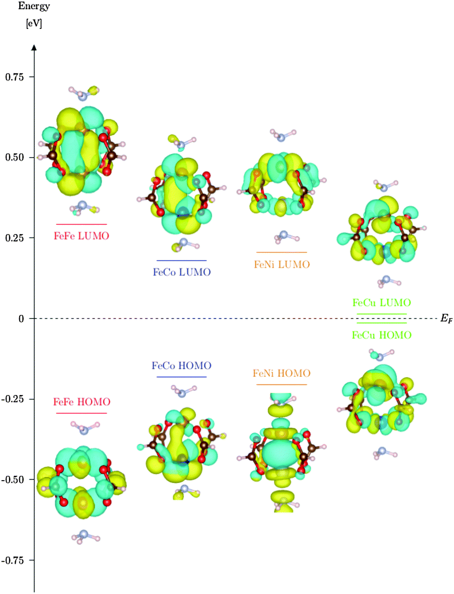Fig. 3 Energy level diagram of the Fe HS SBU family. Electronic structure of the HOMO and LUMO level is visualized with respective wave function plots. Investigated with the NRLMOL code.

Fig. 4 Spin-polarized density of states (DOS) of the Fe HS SBUs calculated with NRLMOL. Spin-up states are displayed in the upper part of the DOS, while spin-down states are in the lower part. The label TDOS stands for total DOS, PDOS for partial DOS, A/B for the metal centers, d for d states and E_F for the Fermi level.

Conversely, the model systems M1-[Fe,Cu] shows levels directly at the Fermi energy, where the other HS Fe models do not. In order to investigate this finding further, we carried out some further model calculations using NRLMOL. The model M1 derived from experimental data shows only a two-fold symmetry in the plane orthogonal to the metal center connecting axis. However, the deviation from a four-fold symmetry is rather small. We carried out calculations on a model system with higher four-fold symmetry and found a doubly degenerate state at the Fermi level which was not completely filled. This indicates that the four-fold symmetry is indeed unstable and one would expect lower symmetry to cancel this degeneracy. The states at the Fermi level might be a hint to a metallic SBU and with that to the possibility to construct a metallic MOF (see M1-[Fe,Cu] states at E_F in Fig. 4). However, further investigation in this respect are needed to prove whether such a metallic behaviour occurs in the crystalline structure or not. To investigate the magnetic stability of the HS states we carried out fixed magnetization calculations (see Fig. 5) using FPLO and QE. For each magnetization between the ones for the HS and LS state, the initial spin-orientations per atom were chosen to be either parallel or anti-parallel to each other, thus referring to the spin-polarization in the HS and the LS state, respectively. This was done to take into account different spin-orientations which lead to the same total magnetization. In Fig. 5 we show the energetically more favoured orientation, i.e. min[E(M)_LS,E(M)_HS], as a function of the magnetization for each of the model systems with Fe. In general, the HS state in M1-[Fe,Fe], M1-[Fe,Co] and M1-[Fe,Ni] is the energetically most favoured one, directly followed by the corresponding LS state. All other possible magnetizations in between are less favoured. Thus the HS is clearly the energetically most stable state of all these systems. The only exception is the M1-[Fe,Cu] system, where with FPLO we found an energetically more favored HS state with another magnetization (M = 4 μ_B) than the one we assumed before (M = 5 μ_B). However, the two states are very close in energy (approximately 20 meV difference), thus a nearly double degenerate ground state occurs. QE calculations show this result as well. An explanation for this behaviour might be originated in the electronic configurations of Cu, where a d⁹ or d¹⁰ configuration may occur, corresponding to a Cu(II) or Cu(I) oxidation state, respectively. Thus the combined system with Fe (d⁶), corresponding to a Fe(II) oxidation state, can show both magnetization depending on the given occupation of the d-orbitals of Cu. Most likely both states can be stabilized depending on small changes in the geometry or in a crystalline structure. As already mentioned before, counting the maximum number of unpaired electrons would result in a state with M = 5 μ_B. For that reason we used this in all other calculations. Considering M = 4 μ_B would not change anything qualitatively, but only increase the value of J. When one of the Fe HS SBUs is used for a new MOF, the SBUs would be separated with mechanically rigid and stable bridges from each other and their geometry would be fixed (M1 – organic bridge – M1). With that it might be possible to retain the magnetic as well as the potential metallic behaviour (see M1-[Fe,Cu]) of the SBU inside this MOF.

Fig. 5 Relative energies of the Fe HS SBUs with fixed magnetizations calculated with FPLO and QE. E_min is the energy of the most favourable state for each system. HS and LS mark the high-spin and low-spin states.

4 Conclusions and outlook

A parameter free screening for the determination of HS solutions for the DUT-8(Ni) model system M1 has been performed using DFT. A comparison between different exchange–correlation functionals showed that PBE is sufficient for the calculation of the exchange coupling constant J. Further investigations were carried out for the following HS candidates: M1-[V,V], M1-[Fe,Fe], M1-[Fe,Co], M1-[Fe,Ni] and M1-[Fe,Cu]. For a more detailed discussion of the electronic structure and magnetic stability, the iron containing M1 HS models have been further investigated. The analyzed electronic structure of the Fe family showed that these systems have electronically and magnetically stable HS ground states, which are most favourable concerning different magnetizations. The density of states (DOS) showed that the levels around the Fermi level are clearly dominated by the d-states of the metal centers. As a consequence the electronic structure can be tuned by changing the transition metal centers A/B. In case of M1-[Fe,Cu] there are two magnetizations (M = 4 μ_B and M = 5 μ_B) which are very close in energy. It might be possible to stabilized those two magnetizations in the crystalline nature of a MOF.

To summarize, we have shown that it is possible to find HS SBUs for a given MOF and a stable M1 Fe HS family has been derived for DUT-8(Ni). Furthermore these HS solutions are stable with respect to all magnetizations. We showed that all used DFT codes agree qualitatively as well as quantitatively. Thus it is possible to use the plane wave method for further investigations. Based on the results of this work it should be considered to insert the obtained HS SBUs into the crystalline structure of DUT-8(Ni), either as a complete replacement of the original SBUs to gain a fully ferromagnetic MOF or as a “magnetic doping” by replacing individual SBUs with some HS SBUs to introduce local HS sites. Additional calculations should consider the mechanical and thermal stability of the resulting structures (molecular dynamics and vibrational analysis) and the effect of structural relaxation on the exchange coupling constant. For first insights, we optimized the M1-[Fe,Fe] system and recalculated the coupling constant. We obtain J = 165.1 cm⁻¹ for NRLMOL and J = 167.7 cm⁻¹ for QE, respectively. Thus the magnitude of J only changes slightly due to geometry optimization and the high-spin character of the coupling is kept. Additionally we relaxed the M1-[Fe,Cu] model and the resulting HOMO–LUMO gap does not change significantly. With that the metallic behaviour of this model is stable against relaxation. Further investigations might include the search for a new kind of MOF, where the HS character of the SBUs is retained. An extended search for HS states by considering further transition metals (e.g. 4d elements) might deliver other HS SBUs. Finally it would be interesting for experimentalists to grow MOFs with a Fe HS SBU and rigid organic bridges to find out whether a HS MOF can be constructed.

Acknowledgements

The authors want to thank the group of theoretical physics in Freiberg and of theoretical chemistry in Dresden for fruitful discussions. Especially Volodymyr Bon for providing the experimental structural information of DUT-8(Ni) and our colleague Simon Liebing for advice and hints concerning the NRLMOL code. Further, the ZIH in Dresden for computational time and support and the WeNDeLIB – Werkstoffe mit neuem Design für verbesserte Lithium-Ionen-Batterien (SPP 1473) as well as the ‘Support the Best’ program within the Excellence Initiative of the TU Dresden for funding.

References

1. T. N. Nguyen, K. A. Abboud and G. Christou, Polyhedron, 2016, 103(Part A), 150–156.
2. N. Klein, C. Herzog, M. Sabo, I. Senkovska, J. Getzschmann, S. Paasch, M. R. Lohe, E. Brunner and S. Kaskel, Phys. Chem. Chem. Phys., 2010, 12, 11778–11784.
3. H. C. Hoffmann, B. Assfour, F. Epperlein, N. Klein, S. Paasch, I. Senkovska, S. Kaskel, G. Seifert and E. Brunner, J. Am. Chem. Soc., 2011, 133, 8681–8690.
4. V. Bon, N. Klein, I. Senkovska, A. Heerwig, J. Getzschmann, D. Wallacher, I. Zizak, M. Brzhezinskaya, U. Mueller and S. Kaskel, Phys. Chem. Chem. Phys., 2015, 17, 17471–17479.
5. K. Trepte, S. Schwalbe and G. Seifert, Phys. Chem. Chem. Phys., 2015, 17, 17122–17129.
6. J. P. Perdew and A. Zunger, Phys. Rev. B: Condens. Matter Mater. Phys., 1981, 23, 5048–5079.
7. M. R. Pederson, R. A. Heaton and C. C. Lin, J. Chem. Phys., 1985, 82, 2688–2699.
8. F. Neese, Coord. Chem. Rev., 2009, 253, 526–563.
9. P. Hohenberg and W. Kohn, Phys. Rev., 1964, 136, B864–B871.
10. W. Kohn and L. J. Sham, Phys. Rev., 1965, 140, A1133–A1138.
11. J. Kortus and M. R. Pederson, Phys. Rev. B: Condens. Matter Mater. Phys., 2000, 62, 5755–5759.
12. M. Pederson, K. Jackson and W. Pickett, Phys. Rev. B: Condens. Matter Mater. Phys., 1991, 44, 3891–3899.
13. M. Pederson, D. Porezag, J. Kortus and D. Patton, Phys. Status Solidi B, 2000, 217, 197–218.
14. M. R. Pederson and K. A. Jackson, Phys. Rev. B: Condens. Matter Mater. Phys., 1991, 43, 7312–7315.
15. M. R. Pederson and K. A. Jackson, Phys. Rev. B: Condens. Matter Mater. Phys., 1990, 41, 7453–7461.
16. J. Perdew, J. Chevary, S. Vosko, K. Jackson, M. Pederson, D. Singh and C. Fiolhais, Phys. Rev. B: Condens. Matter Mater. Phys., 1992, 46, 6671–6687.
17. D. Porezag, PhD thesis, TU Chemnitz, Fakultät für Naturwissenschaften, 1997.
18. D. Porezag and M. R. Pederson, Phys. Rev. A: At., Mol., Opt. Phys., 1999, 60, 2840–2847.
19. K. Koepernik and H. Eschrig, Phys. Rev. B: Condens. Matter Mater. Phys., 1999, 59, 1743–1757.
20. F. Neese, Wiley Interdiscip. Rev.: Comput. Mol. Sci., 2012, 2, 73–78.
21. P. Giannozzi, S. Baroni, N. Bonini, M. Calandra, R. Car, C. Cavazzoni, D. Ceresoli, G. Chiarotti, M. Cococcioni, I. Dabo, A. Dal Corso, S. de Gironcoli, S. Fabris, G. Fratesi, R. Gebauer, U. Gerstmann, C. Gougoussis, A. Kokalj, M. Lazzeri, L. Martin-Samos, N. Marzari, F. Mauri, R. Mazzarello, S. Paolini, A. Pasquarello, L. Paulatto, C. Sbraccia, S. Scandolo, G. Sclauzero, A. Seitsonen, A. Smogunov, P. Umari and R. Wentzcovitch, J. Phys.: Condens. Matter, 2009, 21, 395502.
22. J. J. Mortensen, L. B. Hansen and K. W. Jacobsen, Phys. Rev. B: Condens. Matter Mater. Phys., 2005, 71, 1–11.
23. J. P. Perdew, K. Burke and M. Ernzerhof, Phys. Rev. Lett., 1996, 77, 3865–3868.
24. A. D. Becke, Phys. Rev. A: At., Mol., Opt. Phys., 1988, 38, 3098–3100.
25. C. Lee, W. Yang and R. G. Parr, Phys. Rev. B: Condens. Matter Mater. Phys., 1988, 37, 785–789.
26. I. Opahle, K. Koepernik and H. Eschrig, Phys. Rev. B: Condens. Matter Mater. Phys., 1999, 60, 14035–14041.
27. H. Eschrig, The fundamentals of density functional theory, Springer, 1996, vol. 32.
28. P. E. Blöchl, Phys. Rev. B: Condens. Matter Mater. Phys., 1994, 50, 17953–17979.
29. W. Heisenberg, Z. Phys. Chem., 1926, 38, 411–426.
30. P. A. M. Dirac, Proc. R. Soc. A, 1926, 112, 661–677.
31. J. H. Van Vleck, The theory of electric and magnetic susceptibilities, Clarendon Press, Oxford, 1932.
32. K. Yamaguchi, Y. Takahara and T. Fueno, Applied Quantum Chemistry, Springer, 1986, pp. 155–184.
33. T. Soda, Y. Kitagawa, T. Onishi, Y. Takano, Y. Shigeta, H. Nagao, Y. Yoshioka and K. Yamaguchi, Chem. Phys. Lett., 2000, 319, 223–230.
34. A. P. Ginsberg, J. Am. Chem. Soc., 1980, 102, 111–117.
35. L. Noodleman, J. Chem. Phys., 1981, 74, 5737–5743.
36. L. Noodleman and E. R. Davidson, Chem. Phys., 1986, 109, 131–143.
37. A. Bencini and D. Gatteschi, J. Am. Chem. Soc., 1986, 108, 5763–5771.
38. C. Desplanches, E. Ruiz, A. Rodriguez-Fortea and S. Alvarez, J. Am. Chem. Soc., 2002, 124, 5197–5205.
39. F. Weigend and R. Ahlrichs, Phys. Chem. Chem. Phys., 2005, 7, 3297–3305.
40. K. Park and M. R. Pederson, Phys. Rev. B: Condens. Matter Mater. Phys., 2004, 70, 054414.

---

Footnote

† Electronic supplementary information (ESI) available. See DOI: 10.1039/c5cp07662e

---