MolToxPred: small molecule toxicity prediction using machine learning approach

Abstract

Different types of chemicals and products may exhibit various health risks when administered into the human body. For toxicity reasons, the number of new drugs entering the market through the conventional drug development process has been reduced over the years. However, with the advent of big data and artificial intelligence, machine learning techniques have emerged as a potential solution for predicting toxicity and ensuring efficient drug development and chemical safety. An ML model for toxicity prediction can reduce experimental costs and time while addressing ethical concerns by drastically reducing the need for animals and clinical trials. Herein, MolToxPred, an ML-based tool, has been developed using a stacked model approach to predict the potential toxicity of small molecules and metabolites. The stacked model consists of random forest, multi-layer perceptron, and LightGBM as base classifiers and Logistic Regression as the meta classifier. For training and validation purposes, a comprehensive set of toxic and non-toxic molecules is curated. Different structural and physicochemical-based features in the form of molecular descriptors and fingerprints were employed. MolToxPred utilizes a comprehensive feature selection process and optimizes its hyperparameters through Bayesian optimization with stratified 5-fold cross-validation. In the evaluation phase, MolToxPred achieved an AUROC of 87.76% on the test set and 88.84% on an external validation set. The McNemar test was used as the post-hoc test to determine if the stacked models' performance was significantly different compared to the base learners. The developed stacked model outperformed its base classifiers and an existing tool in the literature, reaffirming its better performance. The hypothesis is that the incorporation of a diverse set of data, the subsequent feature selection, and a stacked ensemble approach give MolToxPred the edge over other methods. In addition to this, an attempt has been made to identify structural alerts responsible for endpoints of the Tox21 data to determine the association of a molecule with a plausible downstream pathway of action. MolToxPred may be helpful for drug discovery and regulatory pipelines in pharmaceutical and other industries for in silico toxicity prediction of small molecule candidates.

---

1. Introduction

In the modern world, the exposure of human beings to a plethora of potentially harmful chemicals is a reality of life. Human bodies process chemicals regularly, ranging from pharmaceuticals to food additives and from natural compounds to cosmetic products. Humans are now even prone to agricultural and industrial chemicals such as pesticide residue in food, contaminants in water, and hazardous gases in the air we breathe.¹ People can get exposed to these chemicals simultaneously and/or sequentially through a variety of exposure routes like oral, dermal, or inhalation. Exposure to these chemicals can trigger adverse drug reactions, allergic responses, disruption of the endocrine system, and even disability or morbidity due to carcinogenic pathways and tissue and/or organ damage. The health risk assessment of these chemicals' exposure depends on the dose, frequency, duration, and administration route.² Furthermore, every year, hundreds of new synthetic chemicals are being released into the environment, which are directly or indirectly accumulating in humans.

All the chemical ingredients for human applications are required to meet certain regulatory requirements to be certified as safe for use. The drug discovery process involves various stages from ideation, to lead identification to development to approval. This process, of drug safety assessment, is a crucial but long, expensive, and very complicated process. Clinical trial data from 2010 to 2017 shows that toxicity is attributed to 30% of clinical failures of drug development.³ The conventional process for toxicity identification involves in vivo and in vitro screening techniques. Although these methods have proven to be helpful, they tend to be time-consuming, inefficient, and highly expensive.^2,4,5 The use of animal testing in clinical trials has been under question due to the ethical and accuracy reasons for predicting human toxicity.² This has led to the emergence of in silico approaches for predicting toxicity which can utilize the inherent properties of the molecules.

Computational approaches have proven to be a promising pre-screening technique for a large number of potential molecules being explored through high-throughput screenings.^6–9 In silico approaches have the advantage of predicting toxicity even before the compound is synthesized,¹⁰ saving time and money over traditional toxicity prediction methods. The in silico approach is based on the concept of the “molecular similarity principle”, which suggests that molecules with similar structures will have similar biological activities.¹¹ These methods use the structural and molecular properties of these molecules to extract the most useful information for the prediction of toxicity.^8,12,13

Several in silico methods have been developed for toxicity prediction like structural alerts, read-across, and Quantitative structure–activity relationships (QSAR).¹⁴ Structural alert (SA) is a chemical substructure that is associated with toxicity,¹⁵ it can be an atom or a collection of atoms. These can be determined by using specialized human expertise¹⁶ or statistical analysis of fragmented datasets.¹⁷ SAs are usually used in a rule-based fashion and associate the presence of structural alert or its combination with toxicity.¹⁸ Another method is read-across which uses information from compound(s) with known properties to infer information for other similar uncharacterized compounds of the same chemical category.¹⁹ The similarity of two chemicals can be calculated statistically using different distance metrics like Tanimoto, Euclidean, Hammings, etc¹⁹. Although the read-across method is transparent and easy to implement, read-across uses a small dataset as compared to other methods owing to the small number of analogs for a compound. The interpretation of results can be complex depending on the choice of similarity and strength of similarity.²⁰ QSAR methods make use of multiple types of machine learning algorithms to establish a link between chemical structure and toxicity. Unlike other methods, QSAR can quantify the relationship between structure and toxicity on their physiochemical property basis.²¹ Machine Learning (ML) is one of the most widely used methods for making such predictions. The machine learning algorithms used have the potential to map both linear and non-linear relationships.

Machine Learning has even outperformed animal testing for a few applications like RASAR by Luechtefeld et al. for oral and dermal toxicity, eye and skin irritation, and mutagenicity.²² ML algorithms can be broadly classified into two types – supervised and unsupervised learning. In supervised learning, all data is labeled and the algorithm learns to map the output label from the input data. Unsupervised learning has all the unlabeled data and the algorithm learns the underlying structure of the data. ML can use different algorithms employing a molecule's chemical and structural properties as a feature set for toxicity prediction. Many supervised ML methods have been explored that use these feature sets for toxicity predictions such as ToxiM,¹² DeepTox,⁸ eToxPred,¹³ and ProTox.⁹ One of the most used datasets for these studies is the Tox21 dataset,²³ which is a collection of in vitro toxicity screening results of thousands of chemicals and approved drugs. DeepTox was one of the best-performing methods in this Tox21 challenge.²⁴ It utilizes the potential of a Deep Neural Network (DNN) trained on molecular descriptors and fingerprints to predict the toxicity of nuclear receptor panels and stress response panels. eToxPred is a method to predict the synthetic accessibility and the toxicity of molecules. It employs an extra Tree Classifier to predict the toxicity by using only fingerprints. It uses publicly available datasets like FDA-approved, KEGG Drug,²⁵ TOXNET,²⁶ T3DB,²⁷ and TCM²⁸ for training and testing the model for toxicity. It reports an AUC of 0.82 for the prediction of toxicity.¹³ ToxiM is another tool for the prediction of toxicity of molecules using fingerprints and descriptors as input features. It trains a random forest model on self-curated positive and negative datasets, which even includes human metabolites as non-toxic molecules.¹² The performance is validated using a validation set and reports an accuracy of 93%. But the drawback of ToxiM is that the dataset used for training is limited by the diversity of data and the number of compounds.

There are several computational methods available for toxicity prediction, but their use is restricted either because the tool is not freely available or because the model was trained on extremely specialized data. So, there is still a need for a method that is not only highly accurate but also fast in training and easily deployable in a classical computing environment. Due to advances in both technology and the exploration of chemical space, the amount of data collected in the pharmaceutical sector is increasing exponentially. To effectively handle the immense amount of data in the chemical–biological space, a machine-learning method that can keep pace is essential. Hence, this study proposes a combination of machine learning and cheminformatics approaches to accurately predict molecule toxicity. The approach involves developing a stacked model utilizing three different base models: LightGBM, random forest, and multi-layer perceptron. These models are selected based on their distinct advantages as individual models and their demonstrated effectiveness in previous studies^8,29,30 on toxicity prediction. Model stacking is a popular and successful approach that has been recently applied in many areas of cheminformatics.^31–33 Stacking allows the flexibility of varied base models that can be trained using a variety of algorithms, architectures, and hyperparameter configurations. By leveraging the diverse characteristics and capabilities of these models, the stacking approach aims to achieve enhanced predictive power for the task.

In terms of data, most of the available works use either descriptors or fingerprints (or a single type of fingerprint) for training purposes. The current work is one of the few attempts to combine descriptors and fingerprints to harness the maximum information and predict the toxicity of molecules. Extensive effort has been put into curating the dataset on which the proposed model gets trained and assessed. The data has been compiled from diverse fields like natural products, human metabolites, known drug molecules, potentially hazardous chemicals, aerosols, and synthetic bio-active compounds. Toxicity is one of the primary properties that are assessed by any industry dealing with compounds for human consumption. For that matter, “the structure of a chemical substance implicitly determines its physical and chemical properties and reactivity, and these properties interact with biological systems to determine its biological/toxicological properties”,^34,35 Hence molecular descriptor and fingerprint-based approach is chosen which represents the structural and physicochemical properties of the compound. Additionally, in the current study an attempt is made to make informed predictions regarding the potential endpoints associated with a molecule, by searching for the defined structural alerts within the molecule in question. For identifying structural alerts in this study Tox21 data is considered. The Tox21 compound library has information about 12 biological receptors: a panel of seven nuclear receptors (NR) and five stress response (SR) pathway assays. Data generated from Tox21 has been used to identify compounds that interact with specific toxic pathways, including some not previously known.^36,37 The proposed method, by incorporating the aforementioned factors, aims to handle an ever-increasing number of compounds being tested by pharma and other industries.

The rest of the paper is organized as follows: Section 2 is Materials and Methods. It discusses the dataset i.e. toxic and non-toxic data, the input features i.e. molecular descriptors and fingerprints, and the feature selection methods applied. It further talks about model building and evaluation which describes the Stacked model architecture and the associated classifiers, followed by the proposed workflow and the model evaluation metrics. Section 3 is Results and discussions, which discusses the results of data processing and feature selection, feature importance, the selection of optimal hyperparameters, toxicity label prediction, and discussions. The model was not only compared with a few base model algorithms but also with an existing tool for toxicity prediction. Section 4 is the structural alerts study and Section 5 is Conclusion.

2. Materials and Methods

The quality of the data limits the performance of a machine learning (ML) model. Along with data availability, tuned hyperparameters are an important prerequisite for model performance and reproducibility in modern machine learning algorithms. This section discusses data compilation and curation, pre-processing, descriptor and fingerprint calculation, feature selection, data splitting, learning algorithms, and model evaluation.

2.1 Datasets

The most important aspect of the supervised machine learning algorithm is a labeled dataset. A robust dataset is required as it will govern the model's performance. In the current study, the data from varied sources were collected, curated, and labeled with two classes viz. toxic and non-toxic depending upon their source. The toxic dataset is labeled as one and consists of known toxins, while the non-toxic dataset is labeled as zero and consists of non-toxins. The dataset was initially cleaned to remove duplicates and salts/metals/duplicates/biologicals. The details of the curated dataset have been given in Table 1.

Table 1 Dataset sources used to evaluate the performance of the toxicity prediction tool

Dataset	Size	Usage
FDA approved drugs	3008	Non-toxic
KEGG drug database	3682	Non-toxic
Human metabolites (BiGG model)	1263	Non-toxic
TOXNET	3036	Toxic
T3DB	3689	Toxic

---

2.1.1 Non-toxic data. The non-toxic dataset comprises the drug molecules that have been approved by regulatory bodies i.e. FDA and KEGG drug database²⁵ and the metabolites present in the human body from the RECON1 model in BIGG database.³⁸ The drugs collected from these regulatory databases might have some side effects but considering their therapeutic advantages it qualifies as non-toxic. FDA-approved drugs (1515) were collected from DrugBank³⁹ and the KEGG drug database contains around ∼3682 drugs approved in U.S., Japan, and Europe. As the human metabolites from pathways have not been reported toxic to humans,¹² this data has also been added to the non-toxic molecules. The 1263 human metabolites were retrieved from the RECON1 model in UCSD's BIGG database.³⁸ The rationale behind including the human metabolites is that these are produced by conserved pathways and to date, no reports of toxicity have been reported.

The Tanimoto similarity⁴⁰ coefficient was used to compare the non-toxic molecules from all the sources, and any molecule with a coefficient of more than 0.95 was excluded as it would be redundant to include because of high similarity. The final non-toxic dataset consists of 5933 non-redundant non-toxic molecules.

2.1.2 Toxic data. The toxic dataset contains toxins from two sources (i) 3036 molecules from TOXNET (ii) and 3689 molecules from the Toxin and Toxin Target Database (T3DB) database. The TOXNET data earlier maintained by NIH and NLM has now been moved to HSDB in PubChem. It is an amalgamation of over 15 databases on toxicology, hazardous chemicals, environmental health, and toxic releases.²⁶ T3DB is a collection of common toxins like drugs, pollutants, pesticides, cosmetics, etc., and their specific human target proteins.²⁷ Metals and small peptides were removed from T3DB data for this analysis. Further redundant and similar molecules were removed at a Tanimoto coefficient threshold of 0.95. This resulted in the final 4696 toxic molecules labelled as one.

2.2 Input features

The principal information for predicting toxicity is based on a drug's chemical structure, as molecules with similar structures may have similar toxicological pathways and properties.⁴¹ In the current work, each compound's chemical molecular structure is expressed in Simplified Molecular-Input Line-Entry System (SMILES) format. The SMILES notation of the molecules obtained from various databases was then converted into canonical SMILES i.e. unique SMILES considering the connectivity and chirality of the molecule using the RDKit library.⁴² From this data, a set of 180 random molecules were initially set aside to use as an external validation set for assessing the built model performance later. It was made sure that these molecules are representative of new molecules and don't share much similarity with the train or test set. For computers to understand the chemical structure, it must be represented in a machine-readable format, such as numbers or characters. The molecular descriptors and fingerprints are these mathematical representations of chemicals and serve as the input features for further analysis and predictions. The details of molecular descriptors and fingerprints have been given in the below subsections. This numerical representation of the data helps for the faster processing of the chemical structures data in a high-throughput fashion.

2.2.1 Molecular descriptors. Molecular descriptors are mathematical representations of the molecular properties of compounds/molecules generated by algorithms. These are used to quantitatively define the physical and chemical information of the compounds/molecules.⁴³ The choice of descriptors has a strong influence on the predictive performance of the model. Molecular descriptors can be classified according to dimensionality: 0D, 1D, 2D, 3D, and 4D descriptors. For the purpose of this study 0D, 1D & 2D descriptors have been calculated via RDKit⁴² library in Python. The missing values were substituted with 0 and the infinite values with 1. 0D-descriptors are independent of molecular connectivity and conformations and refer to atom and bond type counts. 1D-descriptors contain information about fragment counts, and their calculation is independent of information on molecule structure. 2D-descriptors are topological descriptors, derived from molecular graphs, and are conformationally independent.⁴⁴ These descriptors have two major categories: (1) physicochemical properties and (2) fraction of a substructure. Examples of these descriptors have been given in Table 2.

Table 2 Type of descriptors with examples

Descriptor	Examples
0D	Bond counts, mol weight, atom counts
1D	Fragment counts, H-bond acceptor/donors, PSA, number of rings
2D	Balaban, Randic, Wiener, BCUT, kappa, chi

---

2.2.2 Molecular fingerprints. Fingerprints are another form of a descriptor in which molecular structures are encoded to a bit string. It is a series of binary digits (bits), representing the presence or absence of a particular substructure in the molecule indicated by 0 and 1 respectively. These are numeric arrays of n bits long, where n depends on the fingerprint algorithm. The PaDELpy library in Python, which is a wrapper for PaDEL-Descriptor⁴⁵ software, has been used to calculate the molecular fingerprints for the input data. The list of fingerprints calculated have been mentioned in Table 4.

2.3 Feature selection

The molecular descriptors and fingerprints have proved its importance as features over the years for predicting various properties^46,47 of the small molecules and not solely toxicity prediction. However, all the molecular features might not be effective for the prediction of the toxicity of the small molecules, and such ineffective features will not only increase the time required for the training but also adversely impact the performance of the model. Feature selection reduces the complexity of a model and makes it easier to interpret. So, this necessitates the use of efficient feature selection methods that can identify and remove irrelevant and redundant information to obtain practical results. The current dataset for the defined problem in this study consists of molecular descriptors which are numeric continuous values & molecular fingerprints which are high-dimension discrete binary values.

As a result, separate univariate feature selection techniques have been used to select fingerprints and descriptors. This aims to select features that are significantly associated with the target variable while removing highly correlated features. This ensures that the selected features capture relevant information about toxicity and minimize multicollinearity, which can improve the performance and interpretability of the model. To carry out feature selection, a cross-validation strategy is implemented, where the dataset is split into training and testing subsets. The feature selection process is performed solely on the training data to prevent any information leakage from the test set, ensuring unbiased results. Stratified k-fold cross-validation is employed, which takes into account the class distribution of the target variable to maintain its proportionality across the folds. The steps involved in feature selection are shown in Fig. 1 and are described in the below subsections.

Fig. 1 The workflow depicts the feature selection techniques applied to the data under stratified 5-fold cross-validation.

2.3.1 Feature selection for molecular fingerprints. To characterize molecular structural properties of compounds, 12 types of molecular fingerprints are generated using PaDELPy, a Python wrapper for PaDEL-Descriptor software.⁴⁵ This representation of the molecular structure through a chain or vector of bits, with a fixed length, can vary from 79 bits to 4860 bits leading to a large feature set. This feature set can affect the reliability of the built model due to the presence of irrelevant and redundant correlated fingerprints. Therefore, to address this issue, each fingerprint type listed in Table 4 (such as the PubChem fingerprint, Estate fingerprint, etc.) has been individually subjected to the feature selection procedure and then combined subsequently for additional model training.

As molecular fingerprints are discrete values, the chi-square method is used to evaluate features individually with respect to classes i.e. toxic or non-toxic in the target variable. It is a statistical test of independence and estimates whether the class label is independent of a feature or not.⁴⁸ Each PaDEL fingerprint has been treated as an individual feature set, and features have been selected separately. The chi-squared test is based on comparing the obtained values of the frequency of a class to the expected frequency of the class. To use the chi-square test for feature selection, the hypotheses are:

• Null Hypothesis H0: feature & Target Variable are not dependent.

• Alternate Hypothesis H1: feature & Target Variable are dependent.

The criterion for accepting or rejecting the null hypothesis is determined by whether the p-value is more or less than the significance level (α) respectively. Due to the execution of multiple hypothesis tests Bonferroni corrections⁴⁹ have been applied over the chi-squared test.

Further to deal with multicollinearity i.e. correlated features which may act as redundant features, Cramer's v-test⁵⁰ is used. Cramer's v-test is a chi-square-based statistic that assesses how strongly two (nominal) categorical variables are associated or dependent on one another.

Cramer's V ranges between 0 ≤ V ≤ 1, the closer V is to 0, the smaller the association between the categorical variables. So highly correlated features i.e. with Cramer's V correlation greater than 0.5 (ref. 51 and 52) were discarded and only small and medium associations were kept. Table 4 lists the features selected for all the fingerprints for further usage in the model.

The feature selection process is integrated with five-fold stratified cross-validation. This helps in performing the feature selection in a more robust and unbiased manner. By repeatedly splitting the training data into training and validation sets, it can be assessed how well the selected features perform across different subsets of the training data.

Within each fold, Bonferroni corrected chi-square test was applied to the training data to select features based on their p-values (<0.05). These selected features in the same fold are then evaluated using Cramer's V test to identify and remove features with high correlations above the threshold of 0.5. Finally, a consensus is determined by considering the occurrence or agreement of each feature across multiple folds. The details of the chi-square test, Bonferroni corrections, and Cramer's v-test are given in ESI.†

2.3.2 Feature selection for molecular descriptors. Molecular descriptors i.e. the molecule level features which comprise structural and physicochemical properties of small molecules are calculated using the RDkit library in Python.⁴² These consist of 208 descriptors which are ‘numerical’ values, that act as feature sets for predicting toxicity. From this vast set of descriptors, those that significantly affect the performance of the model in predicting toxicity have to be selected. The objective is to choose a set of descriptors that can collectively capture the maximum information about the target variable. For this purpose, mutual information statistics have been used for calculating the relationship between each molecular descriptor and toxicity label.

Mutual information describes relationships in terms of uncertainty i.e. entropy. The mutual information (MI) between two quantities is a measure of the extent to which knowledge of one quantity reduces uncertainty about the other. MI is zero when two quantities are independent and higher values for higher dependency. So, the aim is to select features that have higher mutual information w.r.t to target variable toxicity. The MI between continuous variable X and discrete variable Y represents the reduction in the uncertainty of Y i.e. target variable after observing the X. The mutual information has been calculated using the sklearn library in Python. The function used in this library relies on nonparametric methods based on entropy estimation from k-nearest neighbor distances.^53,54 The details and mathematical representation of the M.I. calculations have been described in the ESI.†

After the MI score for each feature X in the train set is computed with stratified five-fold cross-validation, a threshold value of 0.025 is set as a criterion for feature selection. In addition to this, measures have been taken to remove the multicollinearity in the features. This is done using the Pearson correlation⁵⁵ method to remove redundant highly correlated features which could lead to noise in data. So, highly correlated features i.e. with absolute Pearson correlation greater than 0.9 were discarded within the same fold. Similar to molecular fingerprints a consensus is taken across all folds by considering the occurrence of each feature across multiple folds and final features are selected.

2.4 Model building & evaluation

2.4.1 Model stacking. In the current work, the toxicity prediction problem has been treated as a classification task. To improve the overall prediction performance, a stacked model approach has been implemented. This approach leverages the concept of model stacking, which has shown that combining predictions from multiple diverse models can result in better predictions as compared to using models in isolation.⁵⁶

The architecture of the stacked model consists of two or more well-performing models as base models. These base models get trained on the training data and generate prediction probabilities for each label. These predicted probabilities then serve as input features for a meta-classifier. The meta-classifier is trained on the predictions made by the base models using out-of-sample data. The out-of-sample predictions are generated through k-fold cross-validation and have the same size as the original training set. In other words, the data that was not used to train the base models are utilized to train the meta-classifier, enabling it to make predictions based on the collective insights from the base models. In the current study, three base classifiers were employed followed by a meta-classifier. Each of the base classifiers and the meta classifier has been explained in the below subsection.

2.5 Base learners

2.5.1 LightGBM. LightGBM is a gradient-boosting decision tree (GBDT)⁵⁷ method developed by Microsoft in 2017.²⁹ The LightGBM algorithm is considered as a fast and efficient form of GBDT. It is an ensemble model with a decision tree as its base model, which can be trained sequentially. It works on minimizing the prediction error by combining multiple weak learners to form a strong one. The initial tree will, like other gradient boosting algorithms, learn to fit the target variable, and then each new learner will fit the residual (gradient of loss function) of the previous tree, and minimize the residual. This leads to improved accuracy and reduced bias in the predictions. LightGBM splits the tree in a leaf wise-manner (Fig. 2) with a depth limitation strategy as opposed to the conventional level-wise tree building in other boosting algorithms.²⁹ This means that as a tree grows deeper, it concentrates on extending a single branch rather than growing multiple branches. LightGBM can handle categorical data and provides faster training with techniques like gradient-based one-side sampling (GOSS) and exclusive feature bundling (EFB).

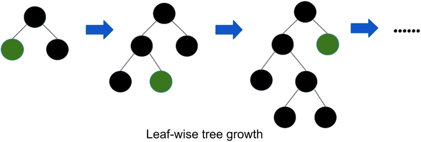Fig. 2 Leaf wise tree growth in LightGBM.⁵⁸

2.5.2 Random forest (RF). Random forest is a decision tree-based ensemble technique, specifically a bagging technique.⁵⁹ Bagging is a technique where several decision trees are trained in parallel followed by aggregation. These parallel trees are built on various subsets of the training dataset using different subsets of available features which helps reduce the variance. These data points and features are chosen at random with a replacement which is called bootstrapping. Bootstrapping ensures that each decision tree in the forest is unique leading to a reduction in the variance of the classifier.⁶⁰ For the classification task, a majority vote is taken of all the decision trees i.e. the most frequent categorical variable will lead to the predicted class.

2.5.3 Multi-layer perceptron (MLP). An MLP is an artificial neural network that consists of at least three interconnected neuron layers: an input layer, a hidden layer, and an output layer. The input layer receives the input data to be processed and the output layer performs the required task of prediction.⁶¹ A number of hidden layers placed between the input and output layers perform the computational task of the MLP using various activation functions. These activation functions introduce non-linearity into the network, allowing it to learn and model complex relationships in the data. The MLP follows a feed-forward architecture, where data flows from the input layer through the hidden layers to the output layer. The neurons within the MLP are trained using the backpropagation algorithm, which adjusts the weights and biases of the neurons to minimize the error between the predicted and actual outputs.⁶²

2.5.4 Logistic regression: meta learner. Logistic regression is employed as the meta learner, it is a simple and efficient statistical method for binary classification problems.⁶³ It uses a logistic function also known as a sigmoid function to return the probability of a label. The output of logistic regression falls within the range of 0 and 1.⁶⁴ In addition, logistic regression does not necessitate a linear relationship between inputs and output variables. Instead, it applies a nonlinear log transformation to the odds ratio. 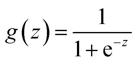The output of logistic regression represents the probability of each class, which is obtained by applying the sigmoid function to the log odds:where g(z) is the probability converted by the sigmoid function and z is log odds in eqn (1).

2.6 Proposed workflow

In the current work, a stacked model-based approach has been taken. The method aims to learn from the feature representations of the small molecules to predict toxicity. The performance of the proposed workflow is evaluated on the curated dataset described in section 2.1. The specific steps for predicting small molecule toxicity using LightGBM are described as follows:

(1) Input datasets: the preprocessed dataset after removing duplicates, missing values, biologicals, and faulty SMILES is used as input for the prediction of toxicity. It contains both non-toxic and toxic molecules, which have been compiled from different sources mentioned in Table 1. Data is divided into training and test set in a ratio of 80 : 20 and normalized. To handle the slight imbalance between the two classes of data, sklearn parameter class weight is set to ‘balanced’ for each of the base learners and meta learner.

(2) Feature extraction and feature selection: features are extracted from the SMILES representation of the molecules in the form of molecular descriptors and fingerprints with the help of RDKit⁴² and PadelPy⁶⁵ libraries respectively in Python. The redundant and highly correlated features are removed, using the feature selection techniques described in Section 2.3.1 and 2.3.2 for molecular fingerprints and descriptors respectively. It is to be noted that feature selection was performed individually for each molecular fingerprint, to select only optimal features and was combined in the end for further predictions. These molecular representations are then used as input for model building.

(3) Hyperparameter tuning: the selection of hyperparameters plays a crucial role in building a model. Hyperparameters are all the parameters that the user can set before training the model to control the learning process. Therefore, to achieve the best performance on the data in a reasonable time, hyperparameter optimization is required. Bayesian optimisation is a method to find the best values of hyperparameters based on the Bayes theorem which will minimize or maximize an objective function. The two main steps include: it builds a probability model i.e. a primary function that assumes the distribution of the objective function which is to be optimized. This prior function, also called the surrogate model, is updated by using an acquisition function. The acquisition function identifies the next input values to evaluate. The goal of Bayesian optimization (eqn (2)) is to find the global maximum or minimum value of function f(x) in the candidate set S and then generate the corresponding best combination of hyperparameters.⁶⁶

X* = arg_x∈Smaxf(x) (2)

where the hyperparameters are input to the function f(x) and maximum metric of choice is set to be output of the function f(x).

For learning a generalized model, the training dataset is randomly divided into five equal parts, in which one part is the independent validation set. The remaining parts were used to train the models and find the best hyperparameters using stratified five-fold cross-validation. The workflow utilizes stratified k-fold cross-validation as it uses stratified sampling which ensures that the ratio of the toxicity label remains the same across original data, training data, and test data. This way a more accurate assessment of performance is achieved by ensuring that no value is over- or underrepresented in the training and test sets. This significantly reduces both bias and variance as most of the data is being used for the training set and validation set respectively.

Hyperparameter optimization is done by performing 10 iterations of Bayesian optimization⁶⁷ with Gaussian processes as a surrogate model and upper confidence bounds as acquisition functions using the scikit BayesOpt⁶⁸ package for eight hyperparameters of LightGBM. For random forest, the HyperOpt⁶⁹ package is used for tuning five hyperparameters by performing 10 iterations, with the Tree-structured Parzen Estimators (TPE) algorithm, which uses the Expected Improvement (EI) as the acquisition function. For Multi Layer Perceptron, BayesOpt⁶⁸ package is used for tuning three hyperparameters of MLP using 10 rounds of optimization with Gaussian processes as a surrogate model.

(4) Model stacking: the best hyperparameters obtained for each base model are then used for training purposes. The stacked model as shown in Fig. 3 has been implemented in the following way:

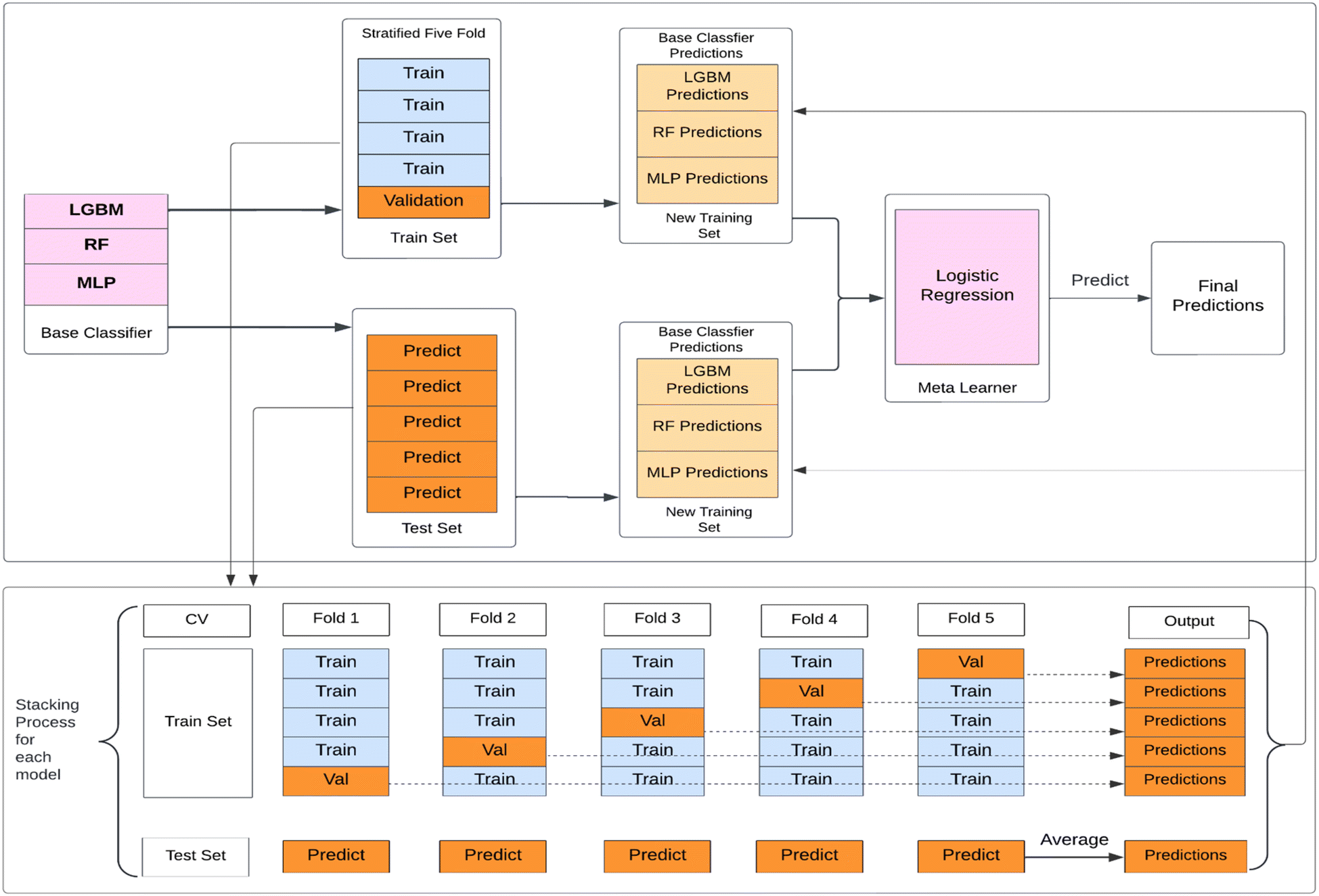Fig. 3 Diagram of the model stacking approach used to predict toxicity target labels. Molecular descriptors and fingerprints are used as input features. Base classifiers: LightGBM, random forest, and multi-layer perceptron. The predicted probabilities from each base classifier are used as input features for the meta classifier: logistic regression. Final predicted label probabilities are output by the logistic regression.

Step 1: the training set for the Stacking Classifier model is divided into five folds using the Stratified five-fold strategy, preserving the percentage of each class. Cross-validation is applied to avoid overfitting. For all base classifiers i.e. LightGBM, RF, and MLP, the training portion of each fold act as a training set, and the predictions are made on the validation portion of each fold.

Step 2: this validation set prediction probabilities from the base models are concatenated, creating a new training set for the meta-classifier. This new training set represents the predictions from all three base models. The original labels are retained as the labels for this dataset.

Step 3: the meta-classifier i.e. Logistic Regression model in this study, combines the predictions made by the base classifiers. The meta-classifier is trained using the new training set and true target variable from the validation portion of the fold. Following that, the meta-classifier is used to make predictions on the test portion of the fold.

Step 4: the predictions from the meta-classifier are collected for each fold, resulting in multiple sets of predictions for the entire test set. The final predictions are calculated by averaging the predictions from all folds.

This process accounts for the variability in predictions across different folds and provides a more robust estimate of the model's performance on unseen data. It helps mitigate overfitting risks and ensures a reliable evaluation of the model's performance.

(5) Model evaluation: to evaluate the quality of the model's predictions, the model is evaluated on various metrics as mentioned in Section 2.7. Accuracy, AUC, Sensitivity, specificity, MCC, and F1 score are calculated for both training and test dataset. External validation data is used to further analyze the stacked model's performance. The stacked model is also compared with the individual base models. A corrected version of McNemar's test is used to assess the statistical significance of the stacked models' performance w.r.t each of the base classifier's performance.

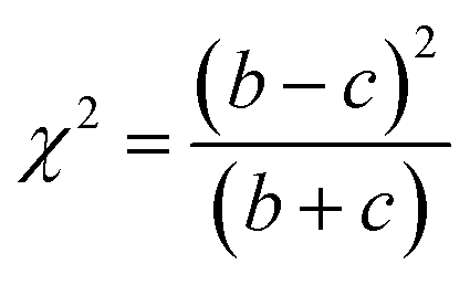
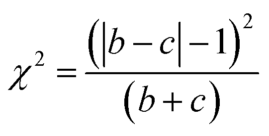
McNemar's test is non-parametric variant of χ² test.⁷⁰ It is based on a 2 times 2 contingency table of the two model's predictions. McNemar's test creates a contingency table that gives the successful and unsuccessful predictions of the two models in question. In Table 3 a sample contingency table has been given, showing b as the number of predictions where model 1 succeeds and model 2 fails, and c as the number of predictions where model 2 succeeds and model 1 fails. If the sum of c and b is sufficiently large, the χ² value follows a chi-squared distribution with one degree of freedom.

Table 3 McNemar's contingency table

	Model2 correct	Model2 wrong
Model1 correct	a	b
Model1 wrong	c	d

---

Then McNemar's formula, corrected for continuity given by Edward et al.,⁷¹ in equation is written as follows:

After setting a significance threshold, here α = 0.05 the p-value is computed, and the p-value is the probability of observing this empirical (or a larger) chi-squared value. If the p-value is lower than the chosen significance level, the null hypothesis can be rejected that there is no significant difference between the performance of the two models. Along with this, the proposed model has also been compared with one of the existing tools ‘eToxPred’ for better comparative assessment.

2.7 Model evaluation

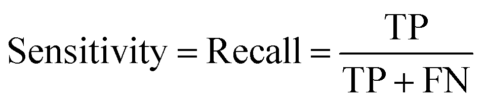
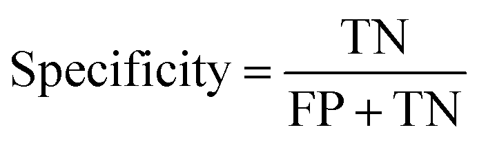
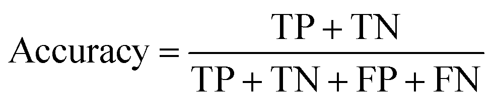
In the context of toxicity binary classification, various metrics are used to assess the performance of the model which are based on the confusion matrix. The confusion matrix comprises True Positives (TP), the number of toxic compounds that are correctly predicted. False Positive (FP), which is the number of non-toxic compounds incorrectly predicted as toxic. True Negatives (TN) refer to the number of correctly predicted non-toxic compounds, and lastly, False Negatives (FN) correspond to the number of incorrectly labeled toxic compounds as non-toxic. The value of sensitivity (recall) eqn (5) reflects the model's ability to correctly predict toxic samples (1), a higher sensitivity value indicates a lower rate of false negatives, indicating that the model is effective in capturing and predicting toxic samples accurately. Whereas the value of specificity eqn (6) represents the model's ability to correctly predict non-toxic samples (0).³⁰ A balance between the two indicates that the model is effective in distinguishing non-toxic samples from toxic ones. Accuracy eqn (7) which is the estimate of the overall performance of the model is also reported, along with the misclassification score. The performance of the classification model across all classification thresholds is represented by the receiver operating characteristic (ROC) curve, which is used to assess a model's robustness. A better metric of evaluation is the area under the curve (AUC), also known as the area under the receiver-operating characteristic (AUROC), for quantifying ROC which is also reported for model performance. This curve is a graphical trade-off between True Positive Rate (TPR) and False Positive Rate (FPR) at different decision thresholds. The probability that a model would score a randomly selected positive sample higher than a randomly selected negative sample is expressed as the area under the ROC curve or AUC. Higher prediction accuracy is indicated by an AUC value that is nearer to 1.¹³ These evaluation metrics were implemented using the scikit learn package⁷² in Python.where, TP = True Positive, TN = True Negative, FP = False Positive, FN = False Negative.

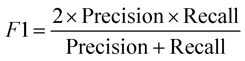
Precision eqn (8) assesses the model's precision in identifying toxic compounds from all the predicted positive cases. Another metric used is the F1 score eqn (9) that combines both precision and recall to provide an overall assessment of the model's performance by taking the harmonic mean of precision in eqn (8) & recall eqn (5). Precision assesses the model's capability in identifying toxic compounds from all the predicted positive cases. While the recall is the proportion of true positive predictions out of all actual positive samples (toxic compounds). A higher F1 score indicates that the model has achieved a good balance between accurately identifying toxic compounds (high precision) and capturing a large proportion of all toxic compounds (high recall). Matthews Correlation Coefficient (MCC) is a metric commonly used to evaluate the performance of binary classification models. It takes into account true positives, true negatives, false positives, and false negatives to provide a balanced measure of the model's overall performance which also has been reported.

3. Results and discussions

3.1 Data processing

In this study, 14 678 compounds were collected from different publicly available databases as described in Table 1. For the initial pre-processing, SMILES are formatted to the canonical SMILES, duplicates are eliminated and redundant, and similar molecules are removed by using a 0.95 threshold of the Tanimoto coefficient. Finally, 10 449 compounds are obtained for use as the training set (8359) and the test set (2090) for the establishment of toxicity prediction models. A separate set of 180 random small molecules is reserved as an external validation set. The Tanimoto similarity scores were computed to determine the degree of similarity between molecules in different sets. In Fig. 4, a value of 0 indicates low similarity and 1 suggests identical molecules. The results show that there is a relatively low degree of similarity between the compounds in both the train–test data and the train–external validation data.

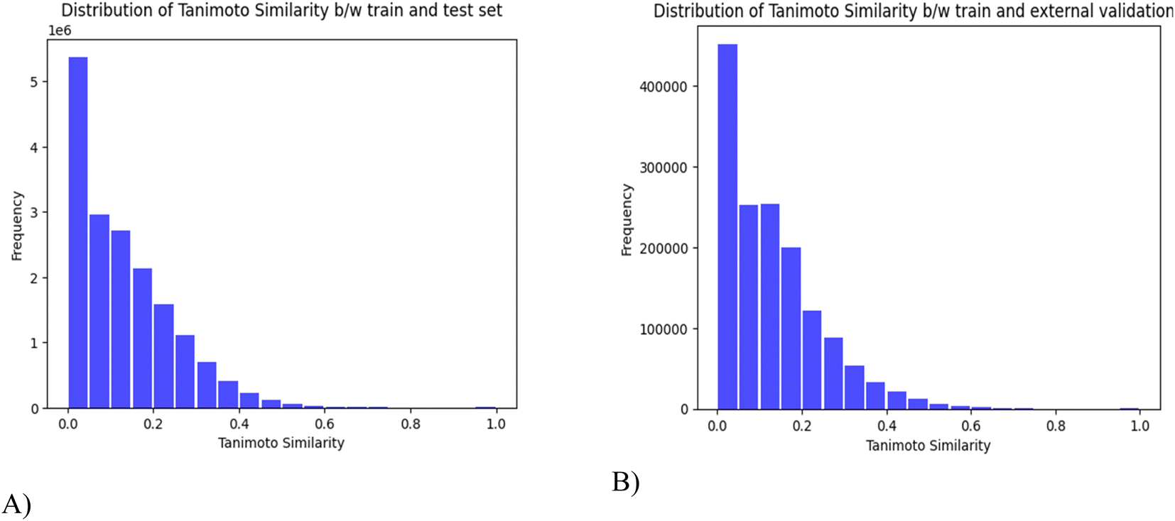Fig. 4 Tanimoto Similarity distributions across (A) Train–Test (B) Train–external validation set.

3.2 Feature selection

The PaDELpy library is used to calculate nine different types of fingerprints and the RDKit library in Python is used to calculate 208 descriptors and Morgan fingerprints. Separate feature selection techniques are applied to descriptors and fingerprints to select features that are effective for the prediction of the toxicity of the small molecules. Therefore, 76 relevant molecular descriptors get selected from 208 descriptors (ESI 2.3.1†) using mutual information and pearson correlation in a stepwise manner as described in Section 2.3.2. Similarly, as described in Section 2.3.1 both the Bonferroni corrected chi-square test and the Cramer's v test, effectively eliminate a large number of redundant and highly correlated fingerprints, yielding 2237 features from 12 193 features as shown in Table 4.

Table 4 Feature selection molecular fingerprints

Fingerprint	Initial count	Selected features
CDK Fingerprint	1024	763
CDK_extended Fingerprint	1024	781
CDK_graphonly fingerprint	1024	184
MACCS Fingerprint	166	54
AtomPairs2D Fingerprint	780	44
Estate Fingerprint	79	29
PubChem Fingerprint	881	73
KlekotaRoth Fingerprint	4860	78
Morgan Fingerprint	2048	193
Substructure Fingerprint	307	38
Combined data	12193	2237

---

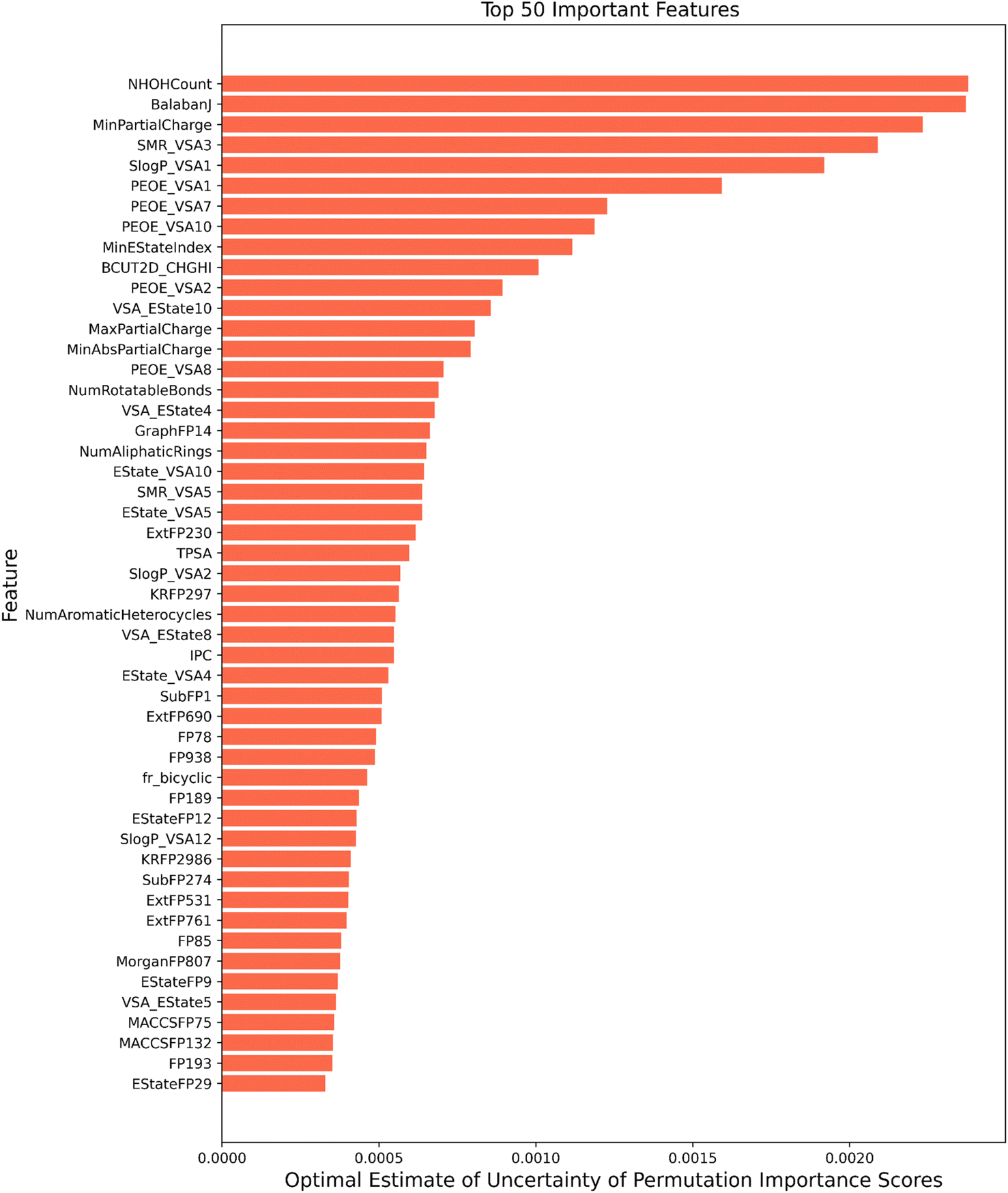
3.3 Feature importance

In order to address the black-box nature of machine learning algorithms and make predictions more explainable, feature importance scores are calculated. Feature importance in predicting the toxicity of a molecule is given through the permutation importance method i.e. the contribution of each feature is calculated in order to predict the target variable. Permutation importance measures the decrease in a model's performance when a single feature (i.e., each key or bit in the molecular fingerprint or each molecular descriptor) is randomly shuffled. If shuffling a feature's values has no effect on the model's predictive performance, it indicates that the feature does not make a significant contribution to the model's predictions. On the other hand, if randomly shuffling the values of a feature leads to a substantial decrease in predictive performance, it suggests that the feature plays a more important role in the model's predictions.⁷³ Each feature is shuffled multiple times and the shuffled feature with the highest performance deviation is the most important and vice versa.

The permutation importance of three individual base classifiers (random forest, MLP, and LightGBM) was calculated with ten times repetition using the test data. Due to the black-box nature of the stacked model,⁷⁴ only individual learners were used to calculate permutation importance.

The systematic and repetitive approach enhances the reliability and confidence in the feature importance assessment, reducing the impact of potential outliers or random fluctuations. To take these repetitions into account in a more robust manner and to understand the influence of the features in each base learner's predictions an optimal estimator from associated uncertainties⁷⁵ is calculated. It is based on the maximum likelihood considerations and the same has been explained in the ESI.† This optimal estimator provides a refined representation of permutation scores, across the three models considering the associated uncertainties from the repeats of permutation. The features highlighted important from this estimate tells about the features contributing to the model's prediction of classifying a molecule as toxic or non-toxic.

Among the feature importance scores generated the top 50 important features according to their optimal estimate of uncertainty have been depicted in Fig. 5 for illustration purposes. Features identified as relevant have been discussed below:

Fig. 5 Top-50 features ranked according to their optimal estimate of uncertainty.

(1) Topological descriptors: topological descriptors are based on a graph representation of the molecule. These take into consideration the internal atomic arrangements of compounds that encode information regarding molecular size, shape, branching, presence of multiple bonds, number of aromatic rings and heteroatoms.⁷⁶ Balbanj⁷⁷ is a distance-based topological descriptor and Ipc index is an information-theory-based topological descriptor.⁷⁸ BCUT 2D metrics take into account bond-type for both adjacent and non-adjacent atoms⁷⁹ is another important topological feature which plays a role in classification. These results of feature importance are in line with a number of toxicity prediction studies on Tox21 (ref. 24) like DeepTox,⁸ and state-of-the-art tools like TOPKAT.⁸⁰ Other findings also show that molecular connectivity indices are an adequate predictive tool for assessing the level of toxicity of a wide range of chemicals.^81,82

(2) Physicochemical descriptors: these consist of the structural and chemical properties of the small molecules. Some of the physicochemical descriptors i.e. min partial charge and max partial charge have the highest feature importance score, these model the distribution of electrons over a molecule. This indicates that electrostatic interactions impact the toxicity profile of the drug. E-state indices play a vital role in toxicity assessment by concurrently encoding the topology and electronic environment of molecular fragments.⁸³ QED (quantitative estimate of drug-likeness)⁸⁴ is a measure of the drug-likeness of a molecule and reflects many properties like molecular weight, octanol/water coefficient logP, topological polar surface area, etc. These properties can affect how a molecule interacts with biological systems and potentially influence its toxicity. NHOH count: number of NHs or Ohs, number of rotatable bonds, number of aliphatic rings and number of aromatic heterocycles are all part of Rdkit's Lipinski parameters of a molecule and found their place in top 50 important features for toxicity prediction. These factors can contribute to toxicity by influencing a molecule's interaction with biological targets, potential nonspecific binding, metabolic stability, and structural characteristics impacting its bioactivity and potential adverse effects.⁸⁵

(3) MOE type descriptors: another set of descriptors that find its place in the top 50 important features are the MOE descriptors. These are numerical features calculated from a connection table representing molecular physical properties, partial charge, along with the surface area contributions. This also includes subdivided surface area descriptors which are based on approximate van der Waals surface area calculation for each atom along with its atomic properties.⁸⁶ These cover contributions to octanol/water coefficient logP (SLogP descriptors) and molecular refractivity (SMR). PEOE descriptors calculate partial charges, which is based on the iterative quantization of atomic orbital electronegativities.⁸⁷ VSA_Estate is the MOE type descriptor using EState indices and surface area contribution. MOE-based descriptors have shown their importance in predicting in silico toxicity in studies by Su et al.,⁸⁸ Jain et al.,⁸⁹ Chavan et al.⁹⁰ and ToxiM.¹²

(4) Molecular fragments and substructures: Fingerprints are a way of encoding the structure of a molecule in a binary form representing the presence or absence of particular substructures. Estate fingerprints (electropological), MACCS fingerprints (cover functional groups, ring systems), Morgan fingerprints (circular), Klekota-Roth fingerprint⁹¹(chemical substructures enriched for biological activity) and graph-based fingerprints are the crucial fingerprints in the top 50 features. Ext fingerprint is an extension of the CDK fingerprint, which takes into account the nature of the ring, including rich structural information⁹² and is a part of the important feature list. These features' importance confirms that the structural and molecular properties of the compound are crucial for learning the relationship between molecules and their toxicity. These fingerprints have also been used repeatedly by several methods in this field by Feng et al.,⁹³ Sharma et al. in ToxiM,¹² and Zhang et al.⁹⁴

3.4 Selection of optimal hyperparameters

3.4.1 LightGBM. The objective function of Bayesian optimization is to maximize the metric ‘AUC’ while finding the best combination of the hyperparameters. The default boosting algorithm used by LightGBM is Gradient Boosting Decision Tree (GBDT). But generally, the gradient-boosting trees suffer from overspecialization i.e. trees added at the later iterations contribute to the prediction of only a few samples and ignore the others. On the other hand, the addition of dropouts in DART (Dropouts meet Multiple Additive Regression Trees) makes it difficult for trees at later iterations to specialize, hence improving performance. Hence, the boosting_type hyperparameter is set to ‘dart’. DART uses dropout similar to the neural network and helps in the regularization of trees.

The eight hyperparameters selected through Bayesian optimization mentioned in Table 5 govern the efficacy and speed of the algorithm. L2 regularization has been applied to determine optimal features through Bayesian optimization without overfitting. The number of leaves (num_leaves) is the maximum number of leaves each weak learner has and is an important parameter that governs the model complexity. The number of leaves should be theoretically less than 2^max_depth, where max depth determines the maximum depth each tree can traverse while still growing leaf-wise.

Table 5 Hyperparameter search space and optimum value for LightGBM using Bayesian optimisation

Hyperparameters	Space	Description	Optimum value
max_depth	(3, 10)	Maximum depth for tree model	10
num_leaves	(31, 40)	Number of leaves	40
learning_rate	(0.001, 0.1)	Learning rate	0.01
min_child_samples	(20, 50)	Minimal number of data in one leaf	32
min_child_weight	(0.001, 0.1)	Minimal sum hessian in one leaf	0.01
subsample	(0.5, 0.9)	Random selection of subset of samples	0.84
colsample_bytree	(0.5, 0.9)	Random selection of subset of features	0.5
lambda_l2	(0.05, 0.8)	L2 regularization	0.8

---

3.4.2 Random Forest. Bayesian Optimization was performed to select the optimal hyperparameters for the random forest classifier while maximizing the accuracy. A set of five hyperparameters and their corresponding search spaces used in the optimization process are mentioned in Table 6 The criterion used for splitting nodes was chosen between ‘entropy’ and ‘gini’. The optimal criterion selected was ‘entropy’. Entropy is a measure of impurity in a set of samples. In the context of random forest, it quantifies the disorder or randomness in the target variable i.e. toxicity label distribution within a node. So, the RF algorithm selects the node that minimizes the entropy impurity. Other hyperparameters include the number of decision trees in a random forest, the depth of each tree, and the minimum number of samples required to split the node.

Table 6 Hyperparameter search space and optimum value for random forest using Bayesian optimisation

Hyperparameters	Space	Description	Optimum value
max_depth	(6, 13)	Maximum depth for tree model	12
min_samples_leaf	(1, 200)	Minimum number of samples in a leaf	11
min_samples_split	(2, 56)	Minimum number of samples required to split an internal node	39
criterion	(‘entropy’, ‘gini')	Minimal number of data in one leaf	‘entropy’
n_estimators	(50, 75, 100, 125,  100, 200, 300, 500)	Number of trees	200

---

3.4.3 Multi layer perceptron. The architecture of the MLP used in this study is as follows:

In the input layer, the number of neurons is set to the number of features for a record in the training data. In this case, the number of neurons in the input layer is 2313; one neuron for each feature. For classification tasks, the number of neurons in the output layer corresponds to the number of class labels. In this model, there is one neuron in the output layer with a sigmoid activation function for the binary classification problem. The MLP classifier used in this model consists of three hidden layers with 1024, 256, and 64 neurons, respectively. These hidden layers apply the rectified linear unit (ReLU) activation function, which introduces non-linearity to the model and helps capture complex patterns in the data. In addition to that three dropout layers are also added to prevent overfitting of the model. The optimizer used for weight optimization is the “Adam” optimizer, a stochastic gradient-based optimizer. The model is trained for a maximum of 10 iterations with a batch size of 32. This means that the model processes the training data in batches of 32 samples per iteration. The complete architecture of the neural network architecture is illustrated in Figure S1.† Furthermore, to mitigate overfitting, additional parameters such as learning rate, dropout rate, and regularization strength are optimized. The details of these are provided in Table 7.

Table 7 Hyperparameter search space and optimum value for multi layer perceptron using Bayesian optimisation

Hyperparameters	Space	Description	Optimum value
learning_rate	(0.001, 0.1)	Step size for adjusting model parameters during training	0.001
dropout_rate	(0.2, 0.5)	Fraction of the input units to drop	0.306
regularization_strength	(1 × 10^−5, 0.01)	Strength of L2 regularization	0.00803

---

3.5 Toxicity label prediction

In order to predict the toxicity of molecules using machine learning, the choice of model is crucial. The proposed method aims to enhance the efficiency and accuracy of toxicity prediction, with a focus on improving the identification of true positive instances while maintaining overall prediction quality. A stacked model approach is employed, which combines multiple base classifiers including random forest (RF), multi-layer perceptron, and LightGBM.

To assess the performance of our stacked model, it is compared against its base classifiers, namely RF, multi-layer perceptron, and LightGBM. Hyperparameters for all the base models are tuned using stratified 5-fold cross-validation on the training data.

By combining bagging and boosting models in a stacked ensemble, the strengths of both techniques are being leveraged. Bagging models help reduce variance and provide stable predictions while boosting models reduce bias and capture complex relationships.⁹⁵ Furthermore, by incorporating a neural network into the stacked model, its strengths in capturing non-linear relationships, feature extraction, and generalization,⁹⁶ lead to improved predictive accuracy and overall model performance.

The prediction results of the test and external validation set under different classifiers are shown in Table 8. In order to evaluate the robustness of the models, ROC and precision–recall curves have been plotted in Fig. 6, which shows the performance of the stacked model as compared to the base classifiers for predicting the toxicity of molecules. Since the stacked model is built on the CV results of its base classifiers, and doesn't have cross-validation results of its own, the test data is used to evaluate and compare its performance with the individual base learners. The AUROC curve in Fig. 6A illustrates that the stacked model outperforms the individual base classifiers, exhibiting a higher AUROC of 87.76% for the test set. This represents a significant improvement compared to the random forest (RF) classifier, which had an AUROC of 1.82% lower, the MLP classifier with an AUROC of 1.58% lower, and the LightGBM classifier with an AUROC of 1.59% lower (AUROC CV results in ESI†). Similarly, for the external validation set, the stacked model achieves an AUROC of 88.84%, surpassing the MLP classifier by 3.76%, the random forest classifier by 2.45%, and the LightGBM classifier by 0.64% as shown in Fig. 6C. These results demonstrate a substantial improvement and further highlight the effectiveness of the developed stacked model in capturing complex patterns and making accurate predictions on unseen data.

Table 8 Comparison results of stacked model & its base classifiers on test and external validation set

Dataset	Method	AUC(%)	ACC(%)	SE (%)	SP(%)	F1 (%)
	Stacked model	87.76	80.91	71.18	88.40	76.43
	LightGBM	86.38	79.14	69.64	86.45	74.38
Test set	MLP	86.39	78.61	61.17	92.04	71.33
	Random forest	86.19	79.47	67.00	89.08	73.95
	Stacked model	88.84	82.22	73.75	89.00	78.67
	LightGBM	88.27	80.56	71.25	88.00	76.51
External validation set	MLP	85.62	81.67	65.00	95.00	75.91
	Random forest	86.71	80.00	68.75	89.00	75.34

---

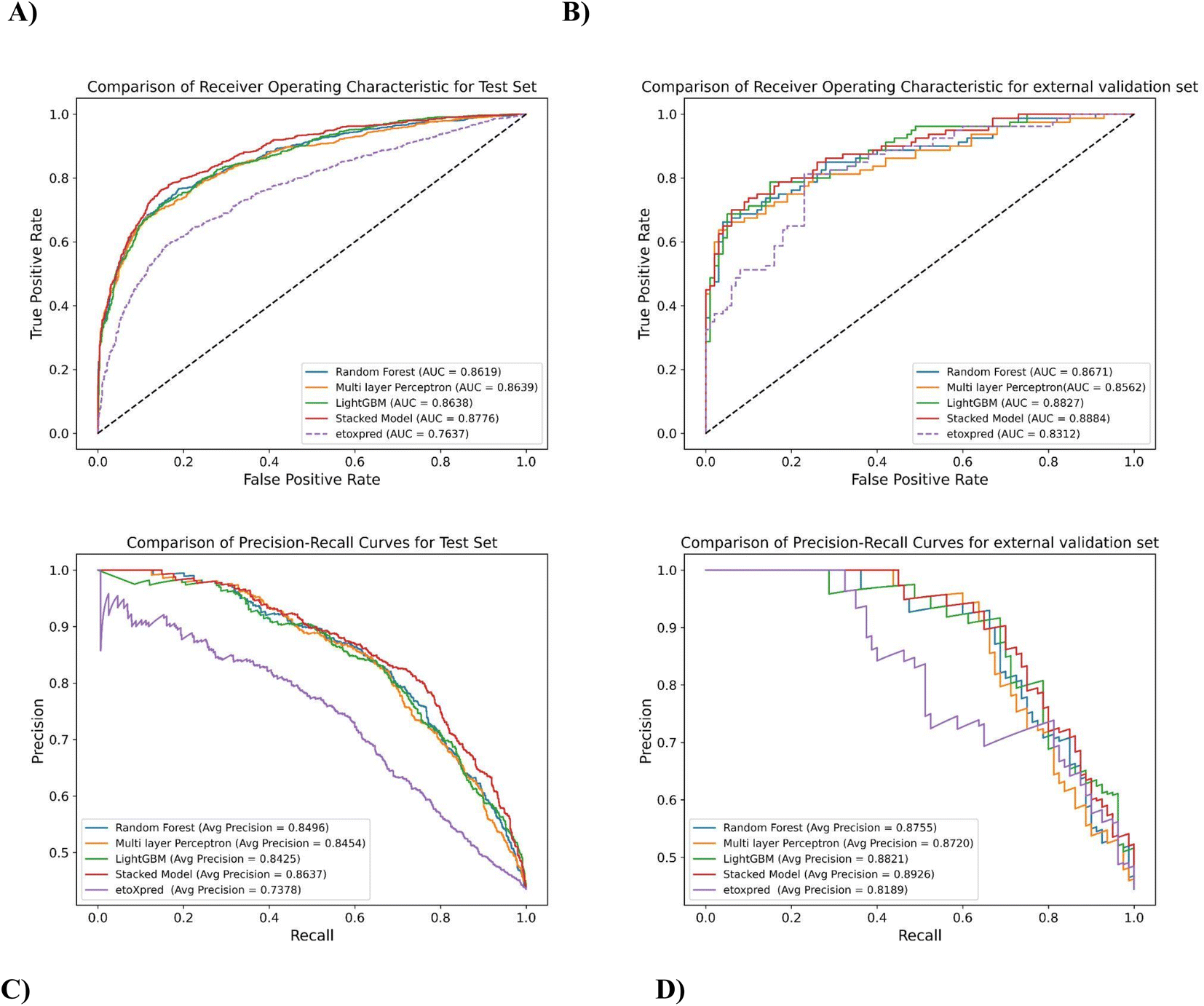Fig. 6 Comparison of ROC and PR curves for different prediction classifiers (A) ROC curves depicting AUROC for different classifiers on test set (B) ROC curves depicting AUROC for different classifiers on the external validation set (C) PR curves depicting AUPRC for different classifiers on the test set (D) PR curves depicting AUPRC for different classifiers on the external validation set.

Fig. 6B and D depicts Area under precision–recall Curve (AUPRC) for both the test set and external validation set, which is based on precision and recall as described in Section 2.7. AUPR is also one of the most robust evaluation metrics and gives the average of precision scores calculated for each recall threshold, giving a better understanding of positive class as compared to negative class. The stacked model achieves an AUPRC of 86.37% on the test set, outperforming the LightGBM classifier by 2.51%, the random forest classifier by 1.65%, and the MLP classifier by 2.16%. The external validation data also follows the same trend, these values indicate that the stacked model has a higher precision–recall trade-off, resulting in better classification performance and a higher proportion of correctly predicted positive instances.

A classification method with high accuracy and precision, and with the lowest misclassification rate, is considered to be the most intelligent classifier for prediction purposes.⁹⁷ In Fig. 7A and B, different metrics like accuracy, F1-score, MCC, specificity, and sensitivity have been reported. When comparing the performance of the stacked model with its base classifiers, it can be observed that the stacked model achieves a higher accuracy of 80.91% for the test set and 82.22% for the external validation set. This is an improvement over the individual base classifiers of LightGBM, MLP, and random forest for the test and external validation set. While accuracy is a commonly used metric for evaluating model performance, it alone may not provide a comprehensive assessment of the model's effectiveness.

Fig. 7 Comparison of accuracy, MCC, F1-score, specificity, and sensitivity for the three base classifiers and stacked model on the (A) test set and (B) external validation set.

For this case, the stacked model achieves an F1 score of 76.43% on the test set and 78.67% on the external validation set indicating that it strikes a good balance between correctly identifying toxic molecules (recall) and avoiding misclassification of non-toxic molecules (precision). This implies that the stacked model performs well in correctly predicting both toxic and non-toxic molecules, reducing both false positives and false negatives.

When comparing the performance of the different models based on the Matthews Correlation Coefficient (MCC), it is observed that the Stacked Model achieves an MCC of 0.61 on the test set, outperforming LightGBM with an MCC of 0.5730, MLP with an MCC of 0.5698, and random forest with an MCC of 0.5816. While for the external validation set, the stacked model also shows competitive performance with an MCC of 0.6396.

In the context of toxicity prediction, sensitivity is crucial as it represents the ability of the model to correctly identify true positive i.e. toxic instances. Therefore, it is essential to evaluate the model's performance not only based on accuracy or MCC but also considering sensitivity to ensure correct predictions of toxic molecules. The stacked model has better sensitivity for both datasets i.e. 0.7118 for the test set and 0.7375 for the external validation set. Additionally, the Stacked Model also exhibits good specificity, which corresponds to the non-toxic class, indicating its ability to accurately classify both toxic and non-toxic molecules. Unlike some instances of the base classifiers that may exhibit bias toward a specific class, the stacked model shows balanced classification performance for both classes.

As can be seen from Table 9 the performance of Stacked Model seems to outperform the base learners. To further evaluate the statistical significance of these results a corrected version of McNemar's test is employed. χ² and p-value have been compared between the stacked model and the base learner models based on McNemar's contingency table. The contingency tables of comparison w.r.t stacked model are mentioned in the ESI.†

Table 9 McNemar's test results

Stacked model vs. model	Chi-squared	P-value
Random forest	7.2500	0.0071
Multi-layer perceptron	14.1603	0.0002
LightGBM	9.1915	0.0024

---

McNemar's statistical analysis supports the finding that the stacked model outperforms random forest, multi-layer perceptron, and LightGBM, as their p-values (Table 9) are below significance level of 0.05, indicating significant differences in performance.

3.6 Comparison with eToxPred

The performance of the proposed method is also compared with an existing publicly available toxicity prediction tool for small molecules i.e. eToxPred.¹³ It employs an Extra Trees Classifier to compute the Tox-score ranging from 0 (low probability of toxicity) to 1 (high probability of toxicity). The model takes SMILES as input and employs molecular fingerprints directly from compounds to predict toxicity. The eToxPred model has been compared with MolToxPred on the test set and the external validation set.

As can be depicted from Fig. 6A and B, on comparison of AUROC scores of the stacked model and eToxPred classifier, the stacked model clearly outperforms in both the cases of the test set and external validation set by 14.91% and 6.88% respectively.

The performance of the stacked model as compared to eToxPred can be further evaluated on various evaluation metrics. eToxPred shows moderate performance on the test set and external validation set, with accuracy ranging from 62.97% to 71.11%. However, when compared to the stacked model, their performance was lower.

In the case of eToxPred, the F1 score is 0.6593 for the test set and 0.73 for the external validation set. These scores suggest a moderate level of accuracy in predicting toxic molecules. However, when these scores are compared with the stacked model's F1 score of 0.7643 for the test set and 0.7867 for the external validation set, it can be clearly seen that the stacked model outperforms the predictive performance of eToxPred. The stacked model demonstrates a better balance between precision and recall, enabling it to effectively predict both toxic and non-toxic molecules.

Although the goal of any toxicity prediction tool is to accurately predict toxic molecules, but it is equally important to have a tool that generalizes well and is not biased towards any particular class. It can be observed that eToxPred seems to be biased towards one class, as evidenced by the sensitivity and specificity values.

The stacked model, on the other hand, demonstrates better performance in terms of sensitivity, specificity, and other metrics. This suggests that the MolToxPred has a more balanced prediction capability and can better generalize to both toxic and non-toxic molecules.

A few test cases have been mentioned here demonstrating MolToxPred outperforming eToxPred. Aflatoxins, which are carcinogenic mycotoxins produced by Aspergillus fungi, have been associated with contamination of the global food supply. Aflatoxin B1 (AFB1), recognized as the most potent natural carcinogen⁹⁸ among these compounds, has been scientifically linked to the development of hepatocellular carcinoma (HCC) in both humans and animals.⁹⁹ Additionally, its hydroxylated metabolite, aflatoxin M1,¹⁰⁰ found in milk and milk products, exhibits similar toxicity to AFB1.¹⁰¹ MolToxPred accurately predicts the toxicity of this class of small molecules with high probability, while eToxPred incorrectly categorizes them as non-toxic.

Oleandrin, a plant metabolite plays a role in traditional medicinal practices¹⁰² to treat various diseases. At the same time, oleandrin is highly toxic and gets easily accumulated in vivo, which may lead to life-threatening intoxication.¹⁰³ It can also cause both gastrointestinal and cardiac effects.¹⁰⁴ While eToxPred misclassifies this plant toxin as non-toxic, MolToxPred accurately predicts its toxicity.

ε-Amanitin is one of the eight Amatoxins found in different genera of poisonous mushrooms, most notably Amanita phalloides. Its mechanism of action involves inhibiting RNA polymerase II, which results in the halting of protein synthesis and disruption of cell metabolism, ultimately leading to cell death.¹⁰⁵ ε-Amanitin is known to cause liver and kidney damage, with the most severe cases being toxic hepatitis characterized by centrilobular necrosis and hepatic steatosis.¹⁰⁶ In terms of toxicity prediction, MolToxPred correctly identifies ε-Amanitin as highly toxic, whereas eToxPred may not provide the same level of accuracy.

4. Towards identifying the correlation between structural alerts and biological pathways for toxicity

The interaction between a chemical compound and the human body can be a complex cascade of different molecular pathways. Understanding the possible relationship between the biological pathway and the substructures that activate a specific characteristic of a molecule, may be helpful in identifying Structural alerts (SAs). Structural alerts are chemical substructures whose presence in compounds is associated with specific types of toxicity/activity. Structural alerts (SAs) based methods are computationally simple and structurally transparent in silico methods to identify the toxic compounds.¹⁰⁷

Typically, methods used to identify structural alerts can be broadly categorized as fragment-based, graph-based, or fingerprint-based approaches. Yang et al.¹⁰⁸ demonstrated that fragment-based methods are more effective in accurately identifying structural alerts within chemical structures. In the current study, SARpy,¹⁷ a recursive fragmentation-based method, has been employed to identify structural alerts for each assay of Tox21 data. Given the training set of molecular structures from each Tox21 assay, with their experimental activity binary labels, SARpy generates every substructure in the set and mines correlations between the incidence of a particular molecular substructure and the activity of the molecules that contain it.¹⁷ Here the target activity label has been set as ‘positive’ for the extraction of structural alerts. In the implementation of SARpy, the fragment size was set to a minimum of 2 and a maximum of 18 atoms. Further to this, a substructure was considered as a SA if it occurs in the minimum of 3 molecules in the dataset for that assay. The precision was set to minimize the false negatives and only the positive rules (active substructures) were extracted with the likelihood ratio threshold of more than 2 for each SA.

These efforts yielded approximately 400 unique SAs across all 12 assays. The specific SAs obtained for each assay are detailed in the ESI in Fig S4–S15.† These SAs may serve as distinctive identifiers for their respective biological pathways. The presence of a particular substructure within a molecule may be helpful in providing a potential correlation with the toxicity-related pathway associated with that molecule.

In order to find an association between a new molecule and any of the Tox21 pathways, substructure matching was conducted on the test set of the Tox21 challenge. This set of 266 molecules encompassed both bioactive molecules with activity in one or more pathways and bioinactive molecules with no activity in any of the pathways across all assays, thereby validating the SAs identified by SARpy from the Tox21 train set.

The substructure-matching results across each assay of the Tox21 test set are mentioned in the ESI.† Across all assays, the test data is aggregated based on whether a molecule exhibits activity in any of the assays within the Tox21 test set. Molecules showing activity are categorized as having a positive label (125), while those consistently showing inactivity across all assays are categorized as having a negative label (171). One critical observation is the relatively high number of True Positives (TP) at 116, signifying the accurate identification of endpoints in molecules because of activity in at least one assay within the Tox21 test set. This is indeed a promising outcome as it demonstrates the approach's ability to detect potentially hazardous compounds effectively. However, it is equally important to address the high number of False Positives (FP) at 150. These false positives represent cases where the algorithm erroneously identified molecules as active when they are, in fact, inactive across all assays. The high number of false positives can also be attributed to the limited number of labeled Tox21 test set. This can also be seen in cases like aniline which is part of FP still, the compound is classified as Group B2, a probable human carcinogen by EPA, and causes serious eye damage and allergic reactions.¹⁰⁹ Similarly phenyldiazene is another SA which is FP here but is present in compounds like pesticide fipronil¹¹⁰ and fungicide Pyraclostrobin which can lead to disrupting CNS activity and secondary hepatotoxicity respectively.^110,111

To improve the overall performance, it is evident that further refinement is required, particularly in reducing the number of false positives. This is where the availability of more labeled data (quantity and quality both) and expert opinion becomes crucial in identifying the relevance of SAs.

The reported structural alerts belong to phenols, aminophenols, furan, and nitroamine and have also been reported by Dang et al.¹¹² Additionally, this study reports the presence of certain halogen derivatives as SA that have also been identified as potential mutagens¹¹³ in the literature. Some small toxic radicals SAs identified in this study like N=N, N–N, N=O, R–O–X, etc. have also been reported by previous studies.¹⁰⁸ Polycyclic aromatic compounds like Anthracene and fluorene have also been identified as SAs. Studies show anthracene and its derivatives bind to estrogen and androgen receptors leading to embryotoxicity.¹¹⁴

It is important to emphasize here that some of the structural alerts are only highlighted here. These structural “alerts” should be regarded as hypotheses for potential undesirable mechanisms rather than strict rules. The generation of structural alerts by SARpy might identify redundant and over specific substructures. Hence more input from experts can help narrow down these SAs, but such approaches can work as providing a head start to pharmaceutical researchers.

5. Conclusion

Before releasing a product for human consumption, the computational toxicity prediction of any compound/molecule aids in the risk assessment procedure for both companies and regulatory bodies. A number of criteria, including compositional, structural, and molecular properties, must be considered when determining a chemical's toxicity. Machine learning-based methods have come to the rescue because these can automatically handle large datasets and perform statistical analysis to find patterns in data. As a result, in this study, a machine learning-based classification workflow was developed to predict the toxicity of molecules using a molecule's structural, molecular, and chemical properties.

The training dataset is curated to represent small molecules that humans come into contact with, such as drugs, metabolites, environmental pollutants, food toxins, and so on, and this dataset plays a role in good model performance. A stacked model was used to take advantage of diverse base classifiers each of which bring its own capabilities. An extensive feature selection method has been implemented to reduce redundant features that do not contribute to the prediction of toxicity. To find the best set of hyperparameters, Bayesian optimization with stratified 5-fold cross-validation was used to avoid overfitting. The tool's effectiveness is validated by reported different evaluation metrics such as AUROC, F1-score, and accuracy in predicting a molecule as toxic or non-toxic. Permutation Importance across the base classifiers has been used to explain the significance of the selected features in predicting toxicity. The developed model's performance was evaluated using both a test set and an external validation set. The proposed method also outperformed the eToxPred tool in terms of performance, which shows this method is at par with existing methods. The performance is attributed to robust data curation: a combination of fingerprints & descriptors, the addition of metabolites and intensive feature selection, and rigorous hyperparameter tuning.

The test and validation set results confirm not only the importance of these properties but also lay the ground for machine learning in toxicity applications. In addition to this, the study also identified a number of structural alerts, shedding light on potential toxic pathways and risks associated with various molecules. These findings can serve as valuable hypotheses for further research, emphasizing the need for expert input to refine and optimize these alerts. One significant challenge when employing AI-based methods and structural-based approaches for drug toxicity prediction is the insufficient availability of high-quality data.^115,116 The development of high-performing models in both AI and structural-based approaches relies on having an ample quantity of training data, coupled with the verification of its quality. Despite the increasing volume of publicly accessible toxicity data, the quality of such data remains a constraining factor. Nevertheless, this workflow will assist the scientific community in determining a molecule's or compound's physiological and environmental toxicity and its association with toxicity related biological pathways before moving forward in the drug development pipeline.

Data availability

The tool and data are available at https://github.com/bioinformatics-cdac/MolToxPred.

Given a new molecule as input the MolToxPred CLI tool, will calculate and provide the probability of the molecule being toxic. This probability score indicates the likelihood that the given molecule may exhibit toxic properties. A higher probability suggests a higher likelihood of toxicity. The output will also include information about the plausible Tox21-based endpoints associated with the molecule.

Conflicts of interest

There are no conflicts of interest to declare.

Acknowledgements

The authors gratefully acknowledge the Ministry of Electronics and Information Technology (MeitY), Government of India, New Delhi, and National Supercomputing Mission (NSM) for providing financial support.

References

1. S. Giri and A. Bader, Drug Discovery Today, 2015, 20, 37–49.
2. G. A. Van Norman, JACC Basic Transl. Sci., 2019, 4, 845–854.
3. D. Sun, W. Gao, H. Hu and S. Zhou, Acta Pharm. Sin. B, 2022, 12, 3049–3062.
4. T. Lavé, N. Parrott, H. Grimm, A. Fleury and M. Reddy, Xenobiotica, 2007, 37, 1295–1310.
5. H. Van de Waterbeemd, Expert Opin. Drug Metab. Toxicol., 2005, 1, 1–4.
6. J. Dong, N.-N. Wang, Z.-J. Yao, L. Zhang, Y. Cheng, D. Ouyang, A.-P. Lu and D.-S. Cao, J. Cheminf., 2018, 10, 29.
7. F. Cheng, W. Li, Y. Zhou, J. Shen, Z. Wu, G. Liu, P. W. Lee and Y. Tang, J. Chem. Inf. Model., 2012, 52, 3099–3105.
8. A. Mayr, G. Klambauer, T. Unterthiner and S. Hochreiter, Front. Environ. Sci., 2016, 3, 80.
9. P. Banerjee, A. O. Eckert, A. K. Schrey and R. Preissner, Nucleic Acids Res., 2018, 46, W257–W263.
10. A. K. Madan, S. Bajaj and H. Dureja, Methods Mol. Biol., 2013, 930, 99–124.
11. M. A. Johnson and G. M. Maggiora, Concepts and Applications of Molecular Similarity, Wiley, 1990.
12. A. K. Sharma, G. N. Srivastava, A. Roy and V. K. Sharma, Front. Pharmacol, 2017, 8, 880.
13. L. Pu, M. Naderi, T. Liu, H.-C. Wu, S. Mukhopadhyay and M. Brylinski, BMC Pharmacol. Toxicol., 2019, 20, 2.
14. J. Hemmerich and G. F. Ecker, Wiley Interdiscip. Rev.: Comput. Mol. Sci., 2020, 10(4), e1475.
15. L. G. Valerio, Toxicol. Appl. Pharmacol., 2009, 241, 356–370.
16. C. A. Marchant, K. A. Briggs and A. Long, Toxicol. Mech. Methods, 2008, 18, 177–187.
17. T. Ferrari, D. Cattaneo, G. Gini, N. Golbamaki Bakhtyari, A. Manganaro and E. Benfenati, SAR QSAR Environ. Res., 2013, 24, 365–383.
18. I. Sushko, E. Salmina, V. A. Potemkin, G. Poda and I. V. Tetko, J. Chem. Inf. Model., 2012, 52, 2310–2316.
19. In Silico Toxicology: Principles and Applications, ed. M. Cronin and J. Madden, Royal Society of Chemistry, Cambridge, 2010.
20. T. W. Schultz, P. Amcoff, E. Berggren, F. Gautier, M. Klaric, D. J. Knight, C. Mahony, M. Schwarz, A. White and M. T. D. Cronin, Regul. Toxicol. Pharmacol., 2015, 72, 586–601.
21. U.S. Environmental Protection Agency, Toxicity Estimation Software Tool (TEST), https://www.epa.gov/chemical-research/toxicity-estimation-software-tool-test#:%7E:text=QSARs%20are%20mathematical%20models%20used,(known%20as%20molecular%20descriptors).
22. T. Luechtefeld, D. Marsh, C. Rowlands and T. Hartung, Toxicol. Sci., 2018, 165, 198–212.
23. R. Huang, M. Xia, D.-T. Nguyen, T. Zhao, S. Sakamuru, J. Zhao, S. A. Shahane, A. Rossoshek and A. Simeonov, Front. Environ. Sci., 2016, 3, 85.
24. Tox21 Data Challenge 2014, https://tripod.nih.gov/tox21/challenge/, accessed 22 May 2022.
25. M. Kanehisa, S. Goto, M. Furumichi, M. Tanabe and M. Hirakawa, Nucleic Acids Res., 2010, 38, D355–D360.
26. G. C. Fonger, D. Stroup, P. L. Thomas and P. Wexler, Toxicol. Ind. Health, 2000, 16, 4–6.
27. D. Wishart, D. Arndt, A. Pon, T. Sajed, A. C. Guo, Y. Djoumbou, C. Knox, M. Wilson, Y. Liang, J. Grant, Y. Liu, S. A. Goldansaz and S. M. Rappaport, Nucleic Acids Res., 2015, 43, D928–D934.
28. C. Y.-C. Chen, PLoS One, 2011, 6, e15939.
29. G. Ke, Q. Meng, T. Finely, T. Wang, W. Chen, W. Ma, Q. Ye and T.-Y. Liu, in Advances in Neural Information Processing Systems 30 (NIP 2017), 2017.
30. G. Idakwo, J. Luttrell, M. Chen, H. Hong, Z. Zhou, P. Gong and C. Zhang, J. Environ. Sci. Health, Part C: Environ. Carcinog. Ecotoxicol. Rev., 2018, 36, 169–191.
31. F. Filias, E. Mylona, K. Blekos, S. Supiot, R. De Crevoisier and O. Acosta, in 2020 IEEE 20th International Conference on Bioinformatics and Bioengineering (BIBE), IEEE, Cincinnati, OH, USA, 2020, pp. 884–889.
32. I. Grenet, K. Merlo, J.-P. Comet, R. Tertiaux, D. Rouquié and F. Dayan, J. Chem. Inf. Model., 2019, 59, 1486–1496.
33. X. Zhu, J. Hu, T. Xiao, S. Huang, Y. Wen and D. Shang, Front. Pharmacol, 2022, 13, 975855.
34. J. D. McKinney, A. Richard, C. Waller, M. C. Newman and F. Gerberick, Toxicol. Sci. Off. J. Soc. Toxicol., 2000, 56, 8–17.
35. K. Roy, S. Kar and R. N. Das, Understanding the Basics of QSAR for Applications in Pharmaceutical Sciences and Risk Assessment, Elsevier/Academic Press, Amsterdam Boston, 2015.
36. S. Chen, J.-H. Hsieh, R. Huang, S. Sakamuru, L.-Y. Hsin, M. Xia, K. R. Shockley, S. Auerbach, N. Kanaya, H. Lu, D. Svoboda, K. L. Witt, B. A. Merrick, C. T. Teng and R. R. Tice, Toxicol. Sci., 2015, 147, 446–457.
37. R. Huang, S. Sakamuru, M. T. Martin, D. M. Reif, R. S. Judson, K. A. Houck, W. Casey, J.-H. Hsieh, K. R. Shockley, P. Ceger, J. Fostel, K. L. Witt, W. Tong, D. M. Rotroff, T. Zhao, P. Shinn, A. Simeonov, D. J. Dix, C. P. Austin, R. J. Kavlock, R. R. Tice and M. Xia, Sci. Rep., 2014, 4, 5664.
38. Z. A. King, J. Lu, A. Dräger, P. Miller, S. Federowicz, J. A. Lerman, A. Ebrahim, B. O. Palsson and N. E. Lewis, Nucleic Acids Res., 2016, 44, D515–D522.
39. D. S. Wishart, C. Knox, A. C. Guo, D. Cheng, S. Shrivastava, D. Tzur, B. Gautam and M. Hassanali, Nucleic Acids Res., 2008, 36, D901–D906.
40. T. T. Tanimoto, in An Elementary Mathematical Theory of Classification and Prediction, 1958.
41. J.-C. Li, in 2020 International Conference on Machine Learning and Cybernetics (ICMLC), IEEE, Adelaide, Australia, 2020, pp. 151–157.
42. RDKit: Open-Source Cheminformatics Software, https://www.rdkit.org/.
43. B. Chandrasekaran, S. N. Abed, O. Al-Attraqchi, K. Kuche and R. K. Tekade, in Dosage Form Design Parameters, ed. R. K. Tekade, Academic Press, 2018, pp. 731–755.
44. ADMET for Medicinal Chemists: a Practical Guide, ed. K. Tsaioun and S. A. Kates, Wiley, Hoboken, N.J, 2011.
45. C. W. Yap, J. Comput. Chem., 2011, 32, 1466–1474.
46. S. Nembri, F. Grisoni, V. Consonni and R. Todeschini, Int. J. Mol. Sci., 2016, 17, 914.
47. S. Lee, M. Lee, K.-W. Gyak, S. D. Kim, M.-J. Kim and K. Min, ACS Omega, 2022, 7, 12268–12277.
48. N. Rachburee and W. Punlumjeak, in 2015 7th International Conference on Information Technology and Electrical Engineering (ICITEE), IEEE, Chiang Mai, Thailand, 2015, pp. 420–424.
49. O. J. Dunn, J. Am. Stat. Assoc., 1961, 56, 52–64.
50. A. C. Acock and G. R. Stavig, Soc. Forces, 1979, 57, 1381.
51. J. Cohen, in Statistical Power Analysis for the Behavioral Sciences, Lawrence Erlbaum Associates, New York University New York, Second edn, 1988.
52. D. K. Lee, Korean J. Anesthesiol., 2016, 69, 555.
53. B. C. Ross, PLoS One, 2014, 9, e87357.
54. A. Kraskov, H. Stögbauer and P. Grassberger, Phys. Rev. E: Stat., Nonlinear, Soft Matter Phys., 2004, 69, 066138.
55. J. Benesty, J. Chen, Y. Huang and I. Cohen, in Noise Reduction in Speech Processing, Springer Berlin Heidelberg, Berlin, Heidelberg, 2009, vol. 2, pp. 1–4.
56. D. H. Wolpert, Neural Networks, 1992, 5, 241–259.
57. J. H. Friedman, Ann. Stat., 2001, 29(5), 1189–1232.
58. LightGBM; Python API, https://lightgbm.readthedocs.io/en/latest/Python-Intro.html.
59. G. Biau and E. Scornet, Test, 2016, 25, 197–227.
60. S. Misra and H. Li, in Machine Learning for Subsurface Characterization, Elsevier, 2020, pp. 243–287.
61. S. Abirami and P. Chitra, in Advances in Computers, Elsevier, 2020, vol. 117, pp. 339–368.
62. J. Li, J. Cheng, J. Shi and F. Huang, in Advances in Computer Science and Information Engineering, ed. D. Jin and S. Lin, Springer Berlin Heidelberg, Berlin, Heidelberg, 2012, vol. 169, pp. 553–558.
63. A. Subasi, in Practical Machine Learning for Data Analysis Using Python, Elsevier, 2020, pp. 91–202.
64. K. Li, H. Xu and X. Liu, Chaos Solit. Fractals., 2022, 157, 111987.
65. T. Kessler and F. Meng, PaDELPy: A Python Wrapper for PaDEL-Descriptor Software (Version 0.1.11), https://github.com/ecrl/padelpy.
66. R. Wang, Y. Liu, X. Ye, Q. Tang, J. Gou, M. Huang and Y. Wen, in 2019 IEEE 3rd Conference on Energy Internet and Energy System Integration (EI2), IEEE, Changsha, China, 2019, pp. 263–268.
67. J. Snoek, H. Larochelle and R. P. Adams, in Advances in Neural Information Processing Systems, ed. F. Pereira, C. J. Burges, L. Bottou and K. Q. Weinberger, Curran Associates, Inc., 2012, vol. 25.
68. R. Martinez-Cantin, J. Mach. Learn. Res., 2014, 15, 3735–3739.
69. J. Bergstra, D. Yamins and D. Cox, in Proceedings of the 30th International Conference on Machine Learning, ed. S. Dasgupta and D. McAllester, PMLR, Atlanta, Georgia, USA, 2013, vol. 28, pp. 115–123.
70. Q. McNemar, Psychometrika, 1947, 12, 153–157.
71. A. L. Edwards, Psychometrika, 1948, 13, 185–187.
72. F. Pedregosa, G. Varoquaux, A. Gramfort, V. Michel, B. Thirion, O. Grisel, M. Blondel, P. Prettenhofer, R. Weiss, V. Dubourg and J. others, Mach. Learn. Res., 2011, 12, 2825–2830.
73. J. Petch, S. Di and W. Nelson, Can. J. Cardiol., 2022, 38, 204–213.
74. M. Shahhosseini, G. Hu, I. Huber and S. V. Archontoulis, Sci. Rep., 2021, 11, 1606.
75. J. D. Chodera, W. C. Swope, J. W. Pitera, C. Seok and K. A. Dill, J. Chem. Theory Comput., 2007, 3, 26–41.
76. R. Gozalbes, J. P. Doucet and F. Derouin, Curr. Drug Targets Infect. Disord., 2002, 2, 93–102.
77. A. Balaban, MATCH Commun. Math. Comput. Chem., 1986, 21, 115–122.
78. D. Bonchev and N. Trinajstić, J. Chem. Phys., 1977, 67, 4517–4533.
79. R. S. Pearlman and K. M. Smith, J. Chem. Inf. Comput. Sci., 1999, 39, 28–35.
80. BIovia Discovery Studio (TOPKAT: TOxicity Prediction by Komputer Assisted Technology)https://www.3ds.com/products-services/biovia/.
81. N. O. Eddy, Sci. Afr., 2020, 10, e00587.
82. M. Protić and A. Sabljić, Aquat. Toxicol., 1989, 14, 47–64.
83. K. Roy and I. Mitra, Curr. Comput. Aided-Drug Des., 2012, 8, 135–158.
84. G. R. Bickerton, G. V. Paolini, J. Besnard, S. Muresan and A. L. Hopkins, Nat. Chem., 2012, 4, 90–98.
85. V. Khanna and S. Ranganathan, BMC Bioinf., 2009, 10, S10.
86. Chemical Computing Group, QuaSAR-Descriptor-MOE 2008.10, https://cadaster.eu/sites/cadaster.eu/files/challenge/descr.htm.
87. P. Labute, J. Mol. Graph. Model., 2000, 18, 464–477.
88. B.-H. Su, M. Shen, E. X. Esposito, A. J. Hopfinger and Y. J. Tseng, J. Chem. Inf. Model., 2010, 50, 1304–1318.
89. S. Jain, E. Kotsampasakou and G. F. Ecker, J. Comput. Aided Mol. Des., 2018, 32, 583–590.
90. S. Chavan, R. Friedman and I. A. Nicholls, Int. J. Mol. Sci., 2015, 16, 11659–11677.
91. J. Klekota and F. P. Roth, Bioinformatics, 2008, 24, 2518–2525.
92. Y. Liu, M. Bi, X. Zhang, N. Zhang, G. Sun, Y. Zhou, L. Zhao and R. Zhong, Processes, 2021, 9, 2074.
93. H. Feng, L. Zhang, S. Li, L. Liu, T. Yang, P. Yang, J. Zhao, I. T. Arkin and H. Liu, Toxicol. Lett., 2021, 340, 4–14.
94. L. Zhang, H. Ai, W. Chen, Z. Yin, H. Hu, J. Zhu, J. Zhao, Q. Zhao and H. Liu, Sci. Rep., 2017, 7, 2118.
95. T. Hastie, J. Friedman and R. Tibshirani, The Elements of Statistical Learning: Data Mining, Inference, and Prediction, 2nd edn, 2009.
96. L. Alzubaidi, J. Zhang, A. J. Humaidi, A. Al-Dujaili, Y. Duan, O. Al-Shamma, J. Santamaría, M. A. Fadhel, M. Al-Amidie and L. Farhan, J. Big Data, 2021, 8, 53.
97. R. Panigrahi and S. Borah, in Social Network Analytics, Elsevier, 2019, pp. 1–19.
98. M. W. Trucksess and C. Diaz-Amigo, in Encyclopedia of Environmental Health, Elsevier, 2011, pp. 888–897.
99. B. R. Rushing and M. I. Selim, Food Chem. Toxicol., 2019, 124, 81–100.
100. Aflatoxin M1, http://www.t3db.ca/toxins/T3D3666.
101. Aflatoxin B1, http://www.t3db.ca/toxins/T3D3598.
102. J. Zhai, X. Dong, F. Yan, H. Guo and J. Yang, Front. Pharmacol, 2022, 13, 822726.
103. G. Yang, C. Zhang, R. Zhang, J. Wei, W. MA and Y. Zhang, Herb. Med., 2017, 299–302.
104. S. A. Jortani, R. A. Helm and R. Valdes, Clin. Chem., 1996, 42, 1654–1658.
105. epsilon-Amanitin, http://www.t3db.ca/toxins/T3D3587.
106. epsilon-Amanitin, https://pubchem.ncbi.nlm.nih.gov/compound/30508.
107. H. Yang, C. Lou, W. Li, G. Liu and Y. Tang, Chem. Res. Toxicol., 2020, 33, 1312–1322.
108. H. Yang, J. Li, Z. Wu, W. Li, G. Liu and Y. Tang, Chem. Res. Toxicol., 2017, 30, 1355–1364.
109. Aniline, https://pubchem.ncbi.nlm.nih.gov/compound/6115.
110. Fipronil, https://pubchem.ncbi.nlm.nih.gov/compound/6115.
111. Pyraclostrobin, https://pubchem.ncbi.nlm.nih.gov/compound/6422843#section=Allowable-Tolerances.
112. N. L. Dang, T. B. Hughes, G. P. Miller and S. J. Swamidass, Chem. Res. Toxicol., 2017, 30, 1046–1059.
113. H. Yang, L. Sun, W. Li, G. Liu and Y. Tang, Toxicol. Sci., 2018, 165, 396–407.
114. A. B. Patel, S. Shaikh, K. R. Jain, C. Desai and D. Madamwar, Front. Microbiol., 2020, 11, 562813.
115. K. Rajpoot, N. Desai, H. Koppisetti, M. Tekade, M. C. Sharma, S. K. Behera and R. K. Tekade, in Pharmacokinetics and Toxicokinetic Considerations, Elsevier, 2022, pp. 357–383.
116. A. O. Basile, A. Yahi and N. P. Tatonetti, Trends Pharmacol. Sci., 2019, 40, 624–635.

---

Footnote

† Electronic supplementary information (ESI) available: Details of the mathematical representation of M.I. for descriptors and Cramer's V test for fingerprints, selected descriptors, and plots for confusion matrix (A) test set (B) external validation set for base and stacked model, Cross-validation scores, Substructure matching result metrics on Tox21 test set, Structural alerts that influenced the toxicity of all tox21 assays, McNemar tests contingency tables. See DOI: https://doi.org/10.1039/d3ra07322j

---