Deep learning for chemical reaction prediction

Abstract

Reaction predictor is an application for predicting chemical reactions and reaction pathways. It uses deep learning to predict and rank elementary reactions by first identifying electron sources and sinks, pairing those sources and sinks to propose elementary reactions, and finally ranking the reactions by favorability. Global reactions can be identified by chaining together these elementary reaction predictions. We carefully curated a data set consisting of over 11 000 elementary reactions, covering a broad range of advanced organic chemistry. Using this data for training, we demonstrate an 80% top-5 recovery rate on a separate, challenging benchmark set of reactions drawn from modern organic chemistry literature. A fundamental problem of synthetic chemistry is the identification of unknown products observed via mass spectrometry. Reaction predictor includes a pathway search feature that can help identify such products through multi-target mass search. Finally, we discuss an alternative approach to predicting electron sources and sinks using recurrent neural networks, specifically long short-term memory (LSTM) architectures, operating directly on SMILES strings. This approach has shown promising preliminary results.

---

Design, System, Application

We present reaction predictor, a system for predicting chemical reactions using deep learning. Reactions are predicted at the level of elementary mechanistic steps, and these predictions can be chained together to yield complex global reactions. Additionally, when given a set of starting materials and target masses, the system can search for unidentified products and suggest possible structures. Reaction predictor's design is modular in such a way that its predictions are readily interpretable. We can tell how it has made a prediction, and why, by following the sequence of elementary reaction steps involved. Reaction predictor uses our own carefully developed data set for training, and continues to improve as more data becomes available.

1 Introduction

Achieving human-level performance at predicting chemical reactions remains an open problem with broad potential applications. Historically there have been three major categories of approaches to reaction prediction: rule-based expert systems, quantum-mechanical simulations, and machine learning-based systems.

Rule-based approaches to reaction prediction^1–3 can be fast, but the requisite systems of manually-implemented rules and exceptions require painstaking maintenance. While they may provide good results within a limited chemical domain, rule-based systems are constrained by the extent to which a human expert has defined the underlying rules, and no comprehensive system of rules covering all of chemistry currently exists. Rule-based systems do not scale well over the long term as new areas of chemistry are added. Furthermore, these systems typically make predictions at the level of overall chemical transformations. Multi-step reactions are condensed into a single transformation, and information about the elementary arrow-pushing steps comprising the multi-step reaction is not available. Yet these elementary steps are the building blocks for predicting novel multi-step global reactions and identifying side products.

Quantum-mechanical (QM) approaches may theoretically yield accurate results based on physical first principles, but in practice are highly sensitive to operator set-up, and are computationally expensive. Many recent studies involving QM-based prediction of reaction pathways are narrowly limited to a single chemical system.^4–8 A clear benefit of these methods, when successful, is their ability to quantitatively predict important reaction parameters such as free energies, energy barriers, transition states, and reaction rates. Still, they require considerable human intervention and are not suitable for making high-throughput predictions.

Machine learning (ML) approaches^9–11 are fast and scalable, but ideally require large data sets from which to learn. Obtaining such chemical data sets is a significant challenge, as many are proprietary and not readily available for academic use. Furthermore, reactions may be unbalanced or not atom-mapped, complicating attempts at statistical learning. Nonetheless, the ML approach to reaction prediction remains promising, and recent advances in deep learning have opened the door to further performance gains.

We also note that these three approaches can be complementary to one another. Rule-based systems have been used to provide training examples for ML-based systems.⁹ Similarly, ML-based systems can benefit from the implementation of a small number of carefully selected rules. In the case of reaction predictor, such rules are designed to address corner cases or express strong priors about specific products or resonance structures that may be problematic or redundant. Other work has explored using ML-based approaches to predict traditional QM observables like molecular atomization energies and electronic structure properties.^12–14 Recent work in our group demonstrated synergies between the QM- and ML-based approaches.¹⁵ We showed that results from QM modeling can be used to derive new training examples for ML algorithms, creating a closed and automated positive feedback loop that improves the ML system.

Reaction predictor is a deep learning-based approach to reaction prediction that operates at the level of elementary reactions. This is a fundamental design choice that reflects how human experts think about chemical reactions. Each elementary step involves the movement of electrons from an electron source to an electron sink. In summary, given a set of input reactants, the reaction predictor pipeline operates in the following multi-step fashion:

1. Enumerate all possible electron sources and electron sinks within the input reactant molecules.

2. Filter the list of candidate sources and sinks, predicting a smaller list containing only the most reactive sources and sinks.

3. Propose reactions by enumerating all combinations of source-sink pairings.

4. Rank the proposed reactions by favorability.

5. Iterate the above process to identify global reactions, or search for unidentified products.

Here we describe the ML design and methodology underpinning reaction predictor's ML-based predictions. To train our models, we carefully curated a training data set consisting of over 11 000 elementary reactions, covering a broad range of advanced organic chemistry. We tested reaction predictor's performance on a benchmark data set of challenging real-world reactions, and demonstrate a high degree of accuracy. We also compare these results with the performance of an early prototype system that was developed in our group.¹⁰ Finally, we also demonstrate that an alternative approach to predicting electron sources and sinks simply by examining SMILES strings, using a long short-term memory (LSTM) architecture,^16,17 shows promising results.

2 Materials & methods

2.1 Chemical-software interface

Molecules and reactions were represented using SMILES and SMIRKS strings,¹⁸ and the OEChem toolkit¹⁹ was used for chemical computation.

2.2 Data

The unit of our data set is an “elementary reaction”. Each elementary reaction represents an energetically favorable mechanistic step with one transition state, with a single labeled electron source and a single labeled electron sink. An earlier version of the data set was primarily composed of undergraduate organic reactions extracted from Reaction Explorer rules,³ plus a set of 368 reactions from graduate-level organic chemistry texts.^20,21 In total, there were 5551 elementary reactions in the original data set. We note that, internally, reaction predictor has three distinct chemical prediction modes: one for polar, one for radical, and one for pericyclic reactions. Each of these uses its own separate underlying data set and trained predictive models. Here we will discuss the polar data set and models, as they represent the most important type of reactions for reaction predictor.

We used a benchmark data set of 289 elementary reactions taken from challenging multi-step transformations to test the performance of our system. These reactions were chosen from reactions in the literature and inferred from reactions in Strategic Applications of Named Reactions in Organic Synthesis²² to cover a broad range of advanced organic chemistry intended to test the system's ability to generalize on real-world reactions. They are not a subset of the training data.

2.3 Data set development

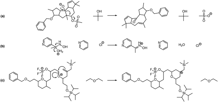
One significant limitation of using Reaction Explorer rules to generate the bulk of the prototype's original training reactions is the inherent bias towards undergraduate chemistry. These training reactions were mostly limited to first, second, and third-row elements. Undergraduate texts often make simplifying assumptions or omit complicating details in order to more clearly present fundamental concepts. A more accurate understanding of the chemical reality is left to be clarified during advanced study. This presents a problem for learning algorithms, which can only learn and generalize based on what they are shown during training. To address this, we reviewed the existing data set in its entirety. Manual inspection of all elementary reactions led to the removal of 884 problematic reactions. Reactions were removed for any of several reasons. First, up to 10% of the elementary reactions were duplicates. Second, some reactions were removed because the arrow-pushing mechanism was depicted incorrectly. Third, some of the training reactions contained products or reactants that were implausible. After removing these problematic reactions, we were left with a cleaned data set of 4667 polar elementary reactions.

Using this cleaned data set as our starting point, we have added 6361 high quality hand-curated reactions: (1) we added about two thousand additional elementary training reactions to cover gaps in various areas of chemistry: phosphorus functional groups, sulfur functional groups, silicon functional groups, tetrahedral intermediates, proton transfers, and migratory displacements. (2) About 1500 additional polar elementary reaction steps were chosen from reaction pathways covered in a first-year graduate course in organic reaction mechanisms including, for example: carbonyl chemistry, enolates, enols, enamines, phosphorus chemistry, sulfur chemistry, allylsilanes, vinylsilanes, strained rings, non-classical carbocations, and others. (3) About a thousand (1004) polar mechanistic steps were sampled from multi-step reaction mechanisms in a well-known book on named reactions.²² (4) About two thousand additional reactions were drawn randomly from the literature and organic chemistry research presentations in an attempt to further complement the data set. Some examples of notable new reaction types added to the data set are shown in Fig. 1. Fig. 1a shows an MPV reduction involving 12 mechanistic steps.²³Fig. 1b represents a Mitsunobu reaction that has seven mechanistic steps.²⁴Fig. 1c shows an eight-step Stetter reaction.²⁵ For each of these examples, critical steps in the reaction mechanism required elementary reactions that were not originally represented in the data set, but have since been added.

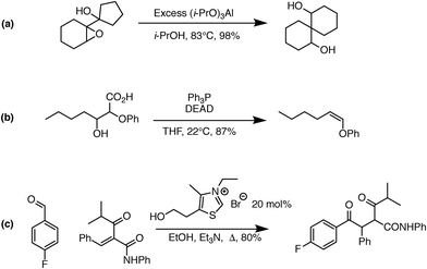Fig. 1 Examples of complex transformations requiring chemistry that was not represented in the original data set. Hand-curated elementary reactions were added to the training data to address these reaction types, and many more, greatly improving predictive capability. Reaction (a) is a 12-step MPV reduction;²³ (b) is a seven-step Mitsunobu reaction;²⁴ and (c) is an eight-step Stetter reaction.²⁵

At time of writing, the total number of elementary reactions in our data set is 11 028. We have observed that the system improves as we grow the data set.

2.4 Combinatorial reaction generation

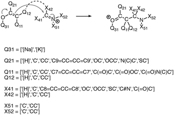
We experimented with using software to automatically generate thousands of additional elementary reactions for our training data set, using the following methodology. First, for a given reaction mechanism, we identified the core molecular template and the appropriate electron movement. We then systematically varied the substituents of the template reaction within realistic chemical constraints to generate all combinations of substitutions. In this way we generated tens of thousands of elementary reactions covering a range of fundamental reaction classes. In order to not overwhelm the existing data with biases towards the combinatorial reactions, we randomly sampled subsets on the order of a thousand reactions for each mechanism. Fig. 2 illustrates this process.

Fig. 2 Illustration of combinatorial reaction generation, including reaction template (top) and substitution constraints (bottom). Thousands of reactions are produced by generating all combinations of allowed substitutions at the Q## and X## sites.

2.5 Applying deep learning

Predicting reactive electron sources and sinks is a crucial step in the reaction predictor pipeline. If the best source or best sink is rejected during the source/sink filtering step, the desired reaction cannot be reproduced. The early prototype of reaction predictor placed great emphasis on recall, with little consideration for precision. That is, the system was biased towards predicting many potential sources and sinks, to avoid missing any, even if most were false positives. Yet false positives have negative performance implications: they significantly increase computation time, which quickly adds up for pathway searches, wherein multiple single-step predictions are chained together to predict products of multi-step reactions. We developed source/sink filtering models focused on both precision and recall, as described below.

For source/sink filtering, we experimented with a variety of architectures, and obtained best results using a single fully-connected feedforward neural network (also called a multilayer perceptron, or MLP) with 1500 inputs, three hidden layers of 200 rectified linear units, and two independent sigmoid output units corresponding to a source prediction and a sink prediction. To avoid overfitting, we use a number of methods including 50% dropout applied to each hidden layer,^26,27 and early stopping. To train the model, weights were initialized as described in Glorot and Bengio,²⁸ and updated using the Adam optimizer²⁹ on mini-batches of 64 examples. An exponentially decaying learning rate, and early stopping based on a validation set of 10% of the training set were used. Models were implemented using Keras and TensorFlow, and training was performed on an NVIDIA Titan X GPU.

We built the training data for our source/sink filtering network as follows. For each elementary reaction in the database, we extracted four training examples of atom reactivity: (1) the labeled source, (2) the labeled sink, and (3, 4) two randomly sampled non-source, non-sink examples. This is illustrated in Fig. 3. There are two advantages to this method compared with the original method of extracting two positively labeled examples (true source and true sink), plus all remaining negative examples. First, we avoid the significant imbalance inherent in the data, as we observe approximately 22-times more negative examples than positive examples. Previously this was addressed by oversampling the positive examples. The second advantage is we avoid adding potentially misleading examples to our training data. Specifically, we avoid negatively-labeled examples that should actually be considered secondary sources or sinks. For a given elementary reaction, the set of atoms not explicitly labeled source or sink contains mostly poor sources and poor sinks. However, some could be considered “second-tier” sources/sinks, either on their own or within a different molecular context. By randomly selecting from these atoms to generate our negative examples, we gain a representative sample of the non-source, non-sink examples in our data, while also avoiding labeling all potential second-tier sources/sinks as negative examples. Extracting the data as described above, our training set for source/sink filtering consisted of 23 850 examples, half of which were positive examples.

Fig. 3 Training examples of atom reactivity extracted for the source/sink filtering network.

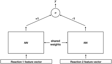
After identifying sources and sinks, and pairing them together, we must rank the resulting set of proposed reactions. To do so, we train a deep Siamese architecture neural network^30,31 to compute a reaction favorability score. Fig. 4 illustrates this architecture. Training examples consist of ordered reaction pairs (R_favorable, R_unfavorable), where the favorable reaction is always presented to the left instance of the shared-weight neural network. Fixed weights of +1 and −1 for left and right outputs are connected to a final sigmoid unit. Thus the final output y approaches 1 if the left reaction was scored higher than the right reaction, and 0 otherwise. After model training, we use one instance of the shared-weight network to compute favorability scores for all reactions, and rank them based on those scores.

Fig. 4 Siamese architecture for reaction ranking. Outputs from the left and right instances of the neural network NN have fixed weights of +1 and −1 into a final sigmoid unit. Thus the final output y approaches 1 if reaction 1 scores higher than reaction 2, and 0 otherwise. We can think of NN as computing a reaction favorability score that is learned by training on many examples of (R_favorable, R_unfavorable) reaction pairs.

For the shared-weight network, we used two hidden layers of 300 tanh units, and a sigmoid output. Initialization and training proceeded as described above for the source/sink models. We generated training examples (R_favorable, R_unfavorable) as follows. For each elementary reaction in the data set, we have one reaction, R_favorable, formed by pairing the labeled electron source with the labeled electron sink. We can propose many additional unfavorable reactions, by pairing the labeled source with all non-sinks, and all non-sources with the labeled sink, within the constraints of chemical feasibility. We use this set of unfavorable reactions to create additional training pairs (R_favorable, R_unfavorable), yielding 387 744 total training examples.

2.6 Feature representation & selection

To make accurate source/sink predictions, we must extract relevant chemical information about each potential source/sink site within a reactant molecule. The features we use to capture this information fall into two categories: physicochemical, and graph-topological. Physicochemical properties are extracted at the atom level. Examples include partial and formal charge, presence and type of filled/unfilled orbitals, presence of lone pairs, and a steric coefficient. Graph-topological features capture properties about the atom and bond connectivity of the molecular graph. These are based on a variation of chemical fingerprints³² and are extracted by enumerating paths and trees over a small neighborhood around a particular atom. Specifically, we allow paths up to depth 6 if the atoms along that path are heteroatoms or are part of a conjugated pi system, otherwise the maximum depth is 3.

Then, to accurately rank reactions by favorability, we must extract reaction-level information that captures both the source/sink interaction and the overall molecular change(s) occurring in the elementary reaction. These reaction-level features include (1) a combination of concatenated source and sink atom-level features, (2) features describing the type of orbitals involved, and (3) net change features, which are created by computing molecular fingerprints for both the reactants and products, then subtracting the reactants fingerprint from the products fingerprint to capture the net changes that occurred during the reaction, e.g. which functional groups and motifs were formed or destroyed.

Extracting the features described above for all examples in our data set yields 293 046 atom-level features, and 62 560 reaction-level features. We select the top 1500 atom-level and top 2000 reaction-level features with the highest mutual information and use those features as the input representations for our source/sink filtering and ranking models.^33,34

2.7 Spectator molecules

A spectator molecule is present on both the reactant and product sides of an elementary reaction, but does not participate in the reaction mechanism. There is information to be gleaned, however, from a spectator molecule's inaction. Each spectator molecule can provide negative source/sink training examples for the filtering model, and unproductive elementary reaction examples for the ranking model. We added the ability to capture and consider these spectator molecules in our training data.

2.8 Offline pathway search

Reaction predictor's pathway search feature allows the user to input starting materials and a set of targets molecule to search for multi-step reaction pathways that yield one or more of the targets. Targets can be specific molecules, masses, or a mixture of both. Users can enter as many search targets as desired for a given set of reactants. This makes pathway search a powerful tool for suggesting alternative reaction pathways and identifying unknown products observed in mass spectrometry data.

2.9 Additional features

While implementing the major features described above, many other improvements were made, including new features and improved chemical capabilities. Here we describe a non-exhaustive selection of these additions.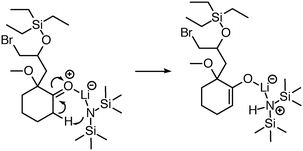

2.9.0.1 Intramolecular reactions. Reaction predictor considers intramolecular reactions in cases where more than a single reactant molecule is present. In the earlier prototype, if two or more reactants were present, only intermolecular reactions were considered. This change is especially important for pathway search, where multiple reactants will either be directly entered or inevitably formed during the course of the search, and to prevent intramolecular reactions at all subsequent steps is to omit a broad swath of potential reactions. Multi-step reaction mechanisms frequently have steps involving intramolecular reactions, and they must be considered, even in the presence of many reactant molecules, in order to achieve high-quality multi-step predictions. Some examples of intramolecular reactions, including a Grob fragmentation, a Neber rearrangement, and an intramolecular Prins reaction, are shown in Fig. 5.^35–37

Fig. 5 Examples of intramolecular reactions that can be predicted by the system. A Grob fragmentation (a), Neber rearrangement (b), and intramolecular Prins reaction (c) are shown. Enabling the prediction of intramolecular reactions when multiple reactants are present significantly increases the number of proposed reactions, but is necessary for the prediction of many reaction pathways including these.

2.9.0.2 “Continue reacting” button for single-step predictions. Users can manually explore a multi-step reaction pathway in a guided stepwise fashion. After submitting reactants and generating a list of predicted products, users can click a button next to any of the results to use those products as the reactants for a new single-step prediction.

2.9.0.3 Improved modeling of alkali metals. The alkali metals Li, Na, and K, are now modeled with a more sophisticated understanding of their bonding potential. Originally, these metals were only allowed to form a single bond, while in reality they can form up to four or more. This is now reflected in reaction predictions involving these atoms. An example involving lithium is shown in Fig. 6.

Fig. 6 Initially, reaction predictor only modeled lithium to include at most one bond. Now the system is capable of correctly predicting this LDA deprotonation to make an enolate via an Ireland transition state.³⁸

2.9.0.4 Additional atom types. Reactants containing Sc, Ti, Zn, As, or Se atoms were not accepted in the early prototype. We have improved the underlying chemical model to be capable of handling these elements. Fig. 7 shows an intermolecular Prins mechanistic step that can be predicted because of the system's ability to model Ti in TiCl₄.

Fig. 7 Reaction predictor can predict this intermolecular Prins mechanistic step because it can model the Ti atom in TiCl₄.³⁹

2.9.0.5 Multiple equivalents for reaction pathways. Reaction predictor can automatically consider an additional equivalent of the reactants at each step of the pathway search before identifying sources and sinks and ranking the resulting combinations. At the early stages of most chemical reactions, the starting materials are present in high concentration relative to other reactive intermediates. Considering additional equivalents of the query reactants allows reaction predictor to anticipate oligomeric products that can be difficult to identify in complex product mixtures. The additional equivalents of the query reactants can also serve in additional mechanistic roles beyond that of substrate, such as catalytic acids or catalytic bases. Addition of the query reactants at each and every step of a pathway search greatly increases the number of potential pathways to be searched and can lead to implausible oligomers. Instead of simply considering the reactants to be present at each and every step, we let the user choose how many equivalents to include. Two examples of reactions requiring multiple equivalents are shown in Fig. 8.

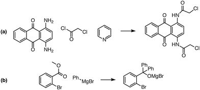Fig. 8 Examples of complex transformations requiring multiple reactant equivalents. In (a), two equivalents of chloroacetyl chloride and pyridine are necessary to complete the double acylation reaction involving six mechanistic steps. In (b), one equivalent of a Grignard reagent adds to the ester, and a second equivalent is needed to add to the ketone that is generated in situ. Reaction predictor is able to predict both of these products from the literature by adding additional reactant equivalents.^40,41

2.9.0.6 ML features. We carefully evaluated the physicochemical and graph-topological features used by our ML algorithms. Some were identified that were either irrelevant or counterproductive for making source/sink predictions. For example, we observed instances where increasing the molecular mass of a molecule, by adding a side-chain to a distant part of the molecule, would cause a source or sink that had at first been predicted correctly, to suddenly be misclassified. We removed this feature, as the reactivity of a candidate source or sink should not be a function of the mass of its parent molecule. We also removed a feature designed to capture whether a source/sink was located centrally or peripherally within the molecular graph, as it too was chemically irrelevant for determining the quality of a source or sink.

3 Results & discussion

3.1 Single-step performance

We assessed single-step reaction prediction performance using the benchmark data set of 289 reactions described above. Table 1 shows the results achieved by reaction predictor.

Table 1 Single-step reaction prediction performance for reaction predictor (RP), compared with the early prototype, using a benchmark data set of 289 reactions

Metric	RP	Prototype
Products recovered	83.0%	58.1%
Products ranked in top-5	80.0%	76.8%
Mean time per reaction (s)	8.3	91.8
Total reactions proposed	20 812	92 158

---

First we note that the early prototype failed while attempting to run the benchmark data set, due to its inability to handle certain atom types, as described above. We incorporated the necessary updated library into that version, so that it could complete the test.

We observe that reaction predictor recovers 83.0% of the expected products anywhere in the ranked list, vs. 58.1% for the prototype. This difference is particularly striking when we consider that the prototype version is biased towards predicting more false positive sources/sinks, in exchange for, ideally, improved recall. We see this reflected in the total number of reactions proposed by each version, with the prototype proposing 92 158 reactions, while our current version proposes 20 812. Yet, even though the prototype predicted so many more reactions, it still only recovered 58.1% of the expected products. That reaction predictor can predict nearly 72 000 fewer reactions while recovering significantly more of the products (83.0%) indicates a dramatic improvement in source/sink filtering capability. We believe this is a result of two factors: the improved breadth and quality of the expanded training data, and the application of deep learning to better learn from that data.

Reaction predictor also performs well in terms of how many correct products are ranked within the top-5 of the ordered reaction list, with 80.0% of correct reactions ranked within the top-5. We have observed that the ranking performance was slower to improve as we grew the training data, compared with source/sink accuracy. Being able to generate hundreds of thousands of training examples for the ranking model, even with only several thousand elementary reactions in the training set, seems to convey enough information to yield a highly accurate trained ranking model. Our observation that doubling the number of elementary reactions in the training set led to a dramatic improvement in source/sink identification, but a relatively minor improvement in ranking performance, seems to imply that the task of source/sink prediction is more difficult than the ranking task. How much of this apparent imbalance is a reflection of chemical reality, versus how much may be an artifact of our particular computational approach and ML design, is unclear. From the perspective of a human chemist, it seems surprising that the source/sink prediction task should be significantly more challenging. We suspect that ultimately the problem is the scarcity of available training data. As more data becomes available, we expect the source/sink predictions to become increasingly accurate.

We also note the significant improvement in average runtime per reaction. For the early prototype, each prediction took 91.8 seconds on average, while reaction predictor is more than ten times faster, averaging 8.3 seconds per reaction. This is a major boon for offline pathway searches, which benefit greatly from faster prediction speed. Results that would have previously taken 10 days can now be processed overnight.

3.2 Combinatorial data

We tested the effect of including combinatorially-generated reactions in our training set by running a direct comparison between a version trained on the standard training set and a version trained on a combinatorially-augmented training set. For this test, the standard training set contained 10 052 elementary reactions, while the combinatorial version contained 36 902 elementary reactions. Decision thresholds were tuned to achieve an equivalent false positive rate for each version, and performance was measured on our benchmark data set of 289 reactions. The results indicated decreased accuracy for the version trained with combinatorial data. Specifically, only 70.2% of the correct products were recovered, and only 70.9% of those recovered were ranked in the top-5, compared with 80.3% and 77.6%, respectively, for the non-combinatorial version. Thus we did not include combinatorial data in the latest reaction predictor training set.

We hypothesize that the homogeneity of the combinatorially-generated reactions introduced biases that degraded predictive performance. We attempted to counteract this by randomly sampling a small fraction of the total reactions generated from each of our combinatorial reaction templates and including only those in the training set. Nonetheless, we observed degraded performance even when the smaller samples of reactions were used in the training set. We believe there is likely value in using combinatorial reaction generation, if done in such a way as to closely mimic the molecular variety observed in real-world reactions. However, the time required to carefully design and validate the necessary templates and constraints, while also aiming to simulate a realistic variety of molecular contexts, is by our estimation better spent simply writing high-quality elementary reactions by hand. For now, we leave combinatorial reaction generation aside for potential future work.

3.3 Pathway search results

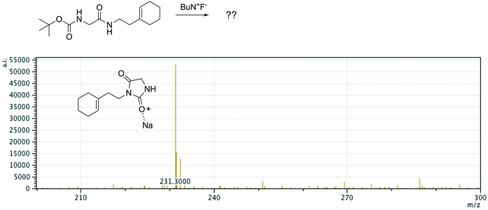
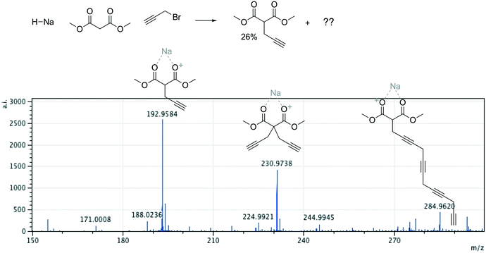
Offline pathway search allows chemists to submit many jobs at once, each one searching for arbitrarily many targets, and have them run in parallel in the background, until results are found and returned via email. The improved performance of our single-step predictions, both in terms of accuracy and speed, make pathway search a powerful tool for understanding unknown masses observed by mass spectrometry, proposing alternative synthesis pathways, or identifying side products.

We submitted a number of pathway search jobs based on actual mass spectrometry data to test the feature's ability to identify unknown peaks. Fig. 9 and 10 illustrate typical instances where pathway search suggested plausible product pathways or structures for unidentified target masses. In Fig. 9, an unexpected product was found after fluoride deprotection.⁴² Pathway search suggested 23 pathways to generate this mass beginning from the actual starting materials used, including the highly plausible imidazolidine-2,4-dione shown. Fig. 10 illustrates a malonate alkylation that generated the desired product in low yield. Pathway search identified a plausible structure corresponding to over-alkylation of the reactant, in effect “troubleshooting” the reaction by suggesting an explanation for the low yield observed.

Fig. 9 A fluoride deprotection afforded an unexpected product with m/z 231. Pathway search found 23 product pathways for the de-sodiated mass, including the highly plausible imidazolidine-2,4-dione shown here.

Fig. 10 A malonate alkylation generated the desired product in low yield. Pathway search generated the expected product, a plausible structure corresponding to over-alkylation, and a third, less plausible structure.

Other times, pathway search may not find a match for a target of interest, or it may find matches that are implausible or were arrived at via implausible mechanisms. These failure modes can be alleviated, to some extent, by adjusting the parameters of the pathway search, which are fully customizable. Users can control the branching factor – how many of the top-ranked reactions are pursued at each search step – as well as the maximum search depth. Even implausible structures matching a target mass may spark ideas or suggest paths to identifying plausible alternatives. Continued improvements to source/sink prediction and ranking accuracy are ultimately the most important factors contributing to pathway search efficacy.

3.4 LSTMs for source and sink prediction

Deep learning and its architectures can be used in many ways. Recurrent neural networks (RNNs), and specifically LSTMs, are deep learning architectures well suited to the translation of variable-length sequences. They are commonly used to translate the written or spoken word from one language to another. We can naturally view chemical reactions as translations from reactants to products. These translations can be considered at the level of elementary reactions, or global transformations, and can be applied in the forward or reverse direction. Thus the “language” being translated is SMILES representations of molecules transforming from reactants into products, or vice versa. Using the inner and outer approach described by P. Baldi,⁴³ we applied bi-directional LSTMs to the problem of translating SMILES strings into source/sink predictions.

Our MLP-based source and sink predictor has some inherent limitations. The input features only cover a limited amount of context for any given molecule, e.g. neighborhoods of atoms within six bonds. Furthermore, these features do not contain any information about other reactants in a given reaction, which could render the prediction task virtually impossible in some cases, where a part of a molecule could act as a sink or a source depending on which other reactants are present.

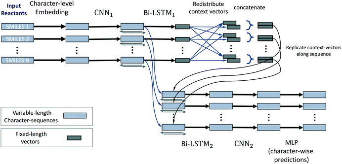
We therefore explore a fundamentally different model to overcome these limitations. On a high level, this model is based on recurrent neural networks that operate on the canonicalized SMILES strings of all reactants. It is able to learn and use features that encode the context of the entire reaction when making predictions for locations of sinks or sources. This model is able to operate on an arbitrary number of reactants of arbitrary size/length† and is invariant to the ordering of reactants as presented. We achieve this invariance by operating on reactants in parallel, and extracting fixed-length feature vectors for all reactants, which are merged into groups of reaction-level features by averaging. A different part of our network uses these reaction-level, and order-invariant, features as context when it predicts sources and sinks for a given molecule.

A more technical description of the model and operating procedure is as follows: SMILES representations of reactants are canonicalized using an implicit representation of hydrogen atoms. We then remove all information that could trivialize the source/sink prediction task. For example, in our data set all potential hydrogen sinks (or sources) appear as the first element in the SMILES string. Thus we remove these and add a ‘start-of-sequence’ character to every SMILES string. The training objective of our model is to predict, for every character in the input SMILES strings of all reactants, whether it corresponds to an atom (or bond) that will act as a sink, source, or both. We further replace multi-letter atoms (e.g. ‘Cu’, ‘Al’) with new unique single characters.

The neural network model conceptually consists of eight elements, shown in Fig. 11. The layers of this model operate on all reactants in parallel, and receive information about the operations on other reactants of the reaction only at the reaction-level-feature merging step (see step 4). The input consists of a variable number (≈ number of reactants) of character strings of variable length (≈ length of individual reactant SMILES). We therefore use zero-padding for mini-batches to speed up training.

Fig. 11 Schematic of the LSTM architecture used for source/sink prediction. This approach operates directly on SMILES strings representing all reactant molecules, and is able to make source/sink predictions using context from the entire set of reactants.

1. The first layer of the neural network maps the input characters into a learned set of vectors (also called embedding), where the number of vectors equals the number of unique characters in all SMILES.

2. This layer is followed by a one-dimensional convolutional neural network (CNN),⁴⁴ and then further by a recurrent bi-directional LSTM.^16,17

3. The layers of the bi-directional LSTM traverse the sequences that correspond to a processed version of the original SMILES strings in the forwards and backwards directions. By doing so they accumulate and compute a fixed-length vector representation of the individual reactants, i.e. learned fingerprint vectors for reactions.

4. These representation vectors are then redistributed across all processing streams of all reactants: a given stream receives the fingerprint of its own molecule and the average of fingerprints of the other molecules/reactants. This way we achieve commutativity of reactants while not mixing contexts of “this” and “other” reactants.

5. These two context vectors are concatenated and replicated across the output of the convolutional layer (2). We thereby re-use the character-level representations that are produced by the convolutional network (for efficiency and to promote weight sharing), while also augmenting them with reaction-level information about all reactants.

6. A bi-directional LSTM, separate from and unrelated to (3), then operates on this augmented stream of vectors and produces one output for each vector. These vectors have a one-to-one correspondence to characters in the input SMILES.

7. The LSTM outputs are then (optionally) processed by a CNN that can refine and sharpen predictions on a local level.

8. A final sequence-distributed MLP then computes the class-probability predictions for each element of a given reactant. These are the character-level predictions of sources/sinks for every atom (or non-atom symbol) in the input SMILES strings, computed for all reactants in parallel.

This model can predict multiple sources/sinks for one reaction or even reactant. We therefore post-process the model's predictions for all reactions by ranking the predicted probabilities, and only using the single most confident source and sink prediction for any given reaction.

The LSTM architecture uses rectified linear units for its hidden layers, and sigmoid outputs. It was trained for 60 epochs on a set of 10 052 labeled SMILES strings. Weights were initialized according to Glorot and Bengio, and updated using the Adam optimizer, with an exponentially decaying learning rate. Training was performed on an NVIDIA Titan X GPU.

To gauge the performance of the LSTM on challenging reactions, we checked its source/sink prediction accuracy on the benchmark data set of 289 reactions, and compared those results with the MLP-based predictor's performance. Table 2 summarizes these results. When we considered only the top-1 highest-scored source and sink, the MLP recovered both correctly in 31.5% of the reactions, while the LSTM recovered both correctly for 29.7% of the reactions. If we consider the top-5 predictions, the MLP recovers both the correct source and the correct sink for 90.0% of the reactions, and the LSTM for 72.4% of them. Similarly, top-10 accuracy for the MLP was 96.9%, and 86.4% for the LSTM. Finally, top-20 accuracy for the MLP was 99.0%, versus 94.6% for the LSTM.

Table 2 MLP and LSTM source/sink prediction accuracy on the benchmark data set of 289 reactions. Predictions were considered correct only if both the true source and the true sink were identified within the top-N ranked source/sink predictions

Top-N accuracy (source & sink)	MLP	LSTM
Top-1	31.5%	29.7%
Top-2	60.2%	51.6%
Top-3	75.8%	63.4%
Top-4	85.8%	68.8%
Top-5	90.0%	72.4%
Top-10	96.9%	86.4%
Top-20	99.0%	94.6%

---

The top-1 score of 29.7% for the LSTM is a promising result, and is particularly impressive as it is comparable to the MLP's top-1 performance of 31.5%. But this result is tempered by the LSTM's lower performance at recovering the labeled sources/sinks within top-5 and top-10 constraints. The crucial job of the source/sink filtering model is to recover all reactive electron sources and sinks, while minimizing the prediction of false positives. Table 2 shows that while the MLP is comparably accurate at predicting a single best source and sink, it is considerably better at recovering the correct sources/sinks, with fewer false positives, when multiple source/sink predictions are allowed. Specifically, the top-2 throughtop-5 scores are 60.2%, 75.8%, 85.8%, and 90.0% for the MLP, vs. 51.6%, 63.4%, 68.8%, and 72.4% for the LSTM. In reality, we expect that a complex chemical reactant will have multiple potentially-reactive source sand sinks, and the MLP recovers those more efficiently than the LSTM. In fact, even if we allow the LSTM to pick its top-10 proposed sources and sinks, its reaction-level accuracy of 86.4% is still lower than the top-5 MLP result of 90.0%. Nonetheless, these results are very promising and indicate potential for using an LSTM architecture for effective source/sink prediction. We emphasize that one advantage of our LSTM approach is its ability to consider the entire context of the reactants when making its source/sink predictions. This capability fundamentally shifts our expectations of what a good source/sink filter should do. Whereas the MLP predicts a set of potentially many reactive sources and sinks, but is necessarily less accurate in choosing the single best ones because it lacks contextual information, the LSTM can see the entire reaction context, and, at least in theory, predict the best source/sink pair given that complete information.

4 Conclusion

Reaction predictor is a unique and powerful tool for predicting chemical reactions at the level of elementary mechanistic steps. Deep learning coupled with a curated and expanded set of training data has yielded significant advances in both speed and predictive accuracy. Importantly, as the data set grows, reaction predictor continues to improve. Pathway search takes advantage of these performance gains to aid in the identification of unknown products by searching in the background and emailing results to the user.

The design of reaction predictor significantly mitigates the “black box” problem of deep learning systems. This refers to the observation that predictions from these systems can be difficult to interpret, if not inscrutable. A hypothetical LSTM making global reaction predictions, for example, has the problem that the “logic” behind any given prediction is obscured, and mistakes are opaque. In contrast, because reaction predictor's design is modular and operates at the level of elementary reactions, we can tell how it has made a prediction, and why, simply by following the sequence of elementary reaction steps involved. Specifically, if reaction predictor makes a mistake in a global reaction, we can look at the underlying elementary step sand identify which step(s) contains an error. And for any erroneous step, we can look at the specific electron sources and sinks that were selected and their rankings in order to narrow down the error and take specific measures to fix it, for instance by adding corrective examples to the training set.

Finally, we demonstrate a promising LSTM-based approach to predicting reactive sites based solely on SMILES strings. This could be used in future work to complement and improve the existing MLP-based source/sink filters. Ultimately we expect reaction predictor will continue to improve over time as new opportunities for refinement are identified, and as more training data becomes available.

Reaction predictor will be made publicly available viahttp://cdb.ics.uci.edu upon acceptance of the paper.

Conflicts of interest

There are no conflicts to declare.

Acknowledgements

We wish to acknowledge DARPA grant HR0011-15-2-0045 to PB; NSF award #1633631; OpenEye Scientific Software and ChemAxon for academic software licenses; and Yuzo Kanomata for computing support.

References

1. J. Gasteiger and C. Jochum, Organic Compunds: Syntheses/Stereochemistry/Reactivity, Springer Berlin Heidelberg, Berlin, Heidelberg, 1978, pp. 93–126.
2. E. S. Blurock, J. Chem. Inf. Comput. Sci., 1995, 35, 607–616.
3. J. H. Chen and P. Baldi, J. Chem. Inf. Model., 2009, 49, 2034–2043.
4. R.-Z. Liao and W. Thiel, J. Chem. Theory Comput., 2012, 8, 3793–3803.
5. I. Polyak, M. T. Reetz and W. Thiel, J. Am. Chem. Soc., 2012, 134, 2732–2741.
6. E. Abad, R. K. Zenn and J. Kästner, J. Phys. Chem. B, 2013, 117, 14238–14246.
7. M. Andrejić and R. A. Mata, J. Chem. Theory Comput., 2014, 10, 5397–5404.
8. M. Shoji, H. Isobe and K. Yamaguchi, Chem. Phys. Lett., 2015, 636, 172–179.
9. M. A. Kayala, C.-A. Azencott, J. H. Chen and P. Baldi, J. Chem. Inf. Model., 2011, 51, 2209–2222.
10. M. A. Kayala and P. Baldi, J. Chem. Inf. Model., 2012, 52, 2526–2540.
11. J. N. Wei, D. Duvenaud and A. Aspuru-Guzik, ACS Cent. Sci., 2016, 2, 725–732.
12. M. Rupp, A. Tkatchenko, K.-R. Müller and O. A. von Lilienfeld, Phys. Rev. Lett., 2012, 108, 058301.
13. K. Hansen, G. Montavon, F. Biegler, S. Fazli, M. Rupp, M. Scheffler, O. A. von Lilienfeld, A. Tkatchenko and K.-R. Müller, J. Chem. Theory Comput., 2013, 9, 3404–3419.
14. J. P. Janet and H. J. Kulik, Chem. Sci., 2017, 8, 5137–5152.
15. P. Sadowski, D. Fooshee, N. Subrahmanya and P. Baldi, J. Chem. Inf. Model., 2016, 56, 2125–2128.
16. S. Hochreiter and J. Schmidhuber, Neural Comput., 1997, 9, 1735–1780.
17. A. Graves and J. Schmidhuber, Neural Netw., 2005, 18, 602–610.
18. C. James, D. Weininger and J. Delany, Daylight theory manual daylight version 4.82, Daylight Chemical Information Systems, 2003.
19. OEChem, version 1.7.4, OpenEye Scientific Software, Inc., Santa Fe, NM, USA, 2012, www.eyesopen.com.
20. R. W. Holman, J. Chem. Educ., 2003, 80, 1259.
21. R. D. Libby, J. Chem. Educ., 2001, 78, 314.
22. L. Kurti and B. Czakó, Strategic applications of named reactions in organic synthesis, Elsevier, 2005.
23. Y. Q. Tu, L. M. Yang and Y. Z. Chen, Chem. Lett., 1998, 27, 285–286.
24. J. Mulzer, A. Pointner, A. Chucholowski and G. Bruntrup, J. Chem. Soc., Chem. Commun., 1979, 52–54.
25. K. L. Baumann, D. E. Butler, C. F. Deering, K. E. Mennen, A. Millar, T. N. Nanninga, C. W. Palmer and B. D. Roth, Tetrahedron Lett., 1992, 33, 2283–2284.
26. G. E. Hinton, N. Srivastava, A. Krizhevsky, I. Sutskever and R. Salakhutdinov, CoRR, 2012, abs/1207.0580.
27. P. Baldi and P. Sadowski, Artificial Intelligence, 2014, 210, 78–122.
28. X. Glorot and Y. Bengio, Proceedings of the Thirteenth International Conference on Artificial Intelligence and Statistics, Chia Laguna Resort, Sardinia, Italy, 2010, pp. 249–256.
29. D. P. Kingma and J. Ba, CoRR, 2014, abs/1412.6980.
30. P. Baldi and Y. Chauvin, Neural Comput., 1993, 5(3), 402–418.
31. J. Bromley, I. Guyon, Y. LeCun, E. Säckinger and R. Shah, Proceedings of the 6th International Conference on Neural Information Processing Systems, San Francisco, CA, USA, 1993, pp. 737–744.
32. S. J. Swamidass, J. Chen, J. Bruand, P. Phung, L. Ralaivola and P. Baldi, Bioinformatics, 2005, 21, i359–i368.
33. A. Kraskov, H. Stögbauer and P. Grassberger, Phys. Rev. E: Stat., Nonlinear, Soft Matter Phys., 2004, 69, 066138.
34. F. Pedregosa, G. Varoquaux, A. Gramfort, V. Michel, B. Thirion, O. Grisel, M. Blondel, P. Prettenhofer, R. Weiss, V. Dubourg, J. Vanderplas, A. Passos, D. Cournapeau, M. Brucher, M. Perrot and E. Duchesnay, J. Mach. Learn. Res., 2011, 12, 2825–2830.
35. L. A. Paquette, J. Yang and Y. O. Long, J. Am. Chem. Soc., 2002, 124, 6542–6543.
36. J. Y. Chung, G.-J. Ho, M. Chartrain, C. Roberge, D. Zhao, J. Leazer, R. Farr, M. Robbins, K. Emerson, D. J. Mathre, J. M. McNamara, D. L. Hughes, E. J. Grabowski and P. J. Reider, Tetrahedron Lett., 1999, 40, 6739–6743.
37. D. J. Kopecky and S. D. Rychnovsky, J. Am. Chem. Soc., 2001, 123, 8420–8421.
38. K. Tanino, K. Onuki, K. Asano, M. Miyashita, T. Nakamura, Y. Takahashi and I. Kuwajima, J. Am. Chem. Soc., 2003, 125, 1498–1500.
39. A. Gomtsyan, R. G. Schmidt, E. K. Bayburt, G. A. Gfesser, E. A. Voight, J. F. Daanen, D. L. Schmidt, M. D. Cowart, H. Liu, R. J. Altenbach, M. E. Kort, B. Clapham, P. B. Cox, A. Shrestha, R. Henry, D. N. Whittern, R. M. Reilly, P. S. Puttfarcken, J.-D. Brederson, P. Song, B. Li, S. M. Huang, H. A. McDonald, T. R. Neelands, S. P. McGaraughty, D. M. Gauvin, S. K. Joshi, P. N. Banfor, J. A. Segreti, M. Shebley, C. R. Faltynek, M. J. Dart and P. R. Kym, J. Med. Chem., 2016, 59, 4926–4947.
40. H.-S. Huang, H.-F. Chiu, A.-L. Lee, C.-L. Guo and C.-L. Yuan, Bioorg. Med. Chem., 2004, 12, 6163–6170.
41. F. Cai, X. Pu, X. Qi, V. Lynch, A. Radha and J. M. Ready, J. Am. Chem. Soc., 2011, 133, 18066–18069.
42. A. D. Mood, I. D. U. A. Premachandra, S. Hiew, F. Wang, K. A. Scott, N. J. Oldenhuis, H. Liu and D. L. Van Vranken, ACS Med. Chem. Lett., 2017, 8, 168–173.
43. P. Baldi, Data Min. Knowl. Discov., 2017, 1–13.
44. Y. LeCun and Y. Bengio, in Y. LeCun and Y. Bengio, ed. M. A. Arbib, MIT Press, Cambridge, MA, USA, 1998, ch. Convolutional Networks for Images, Seech, and Time Series, pp. 255–258.

---

Footnote

† However, we expect that the accuracy of predictions will degrade for reactions with very large molecules.

---