DOI:
10.1039/C7SM01757J
(Paper)
Soft Matter, 2018,
14, 61-72
Growth and relaxation of a ridge on a soft poroelastic substrate
Received
31st August 2017
, Accepted 31st October 2017
First published on 31st October 2017
Abstract
Elastocapillarity describes the deformations of soft materials by surface tensions and is involved in a broad range of applications, from microelectromechanical devices to cell patterning on soft surfaces. Although the vast majority of elastocapillarity experiments are performed on soft gels, because of their tunable mechanical properties, the theoretical interpretation of these data has been so far undertaken solely within the framework of linear elasticity, neglecting the porous nature of gels. We investigate in this work the deformation of a thick poroelastic layer with surface tension subjected to an arbitrary distribution of time-dependent axisymmetric surface forces. Following the derivation of a general analytical solution, we then focus on the specific problem of a liquid drop sitting on a soft poroelastic substrate. We investigate how the deformation and the solvent concentration field evolve in time for various droplet sizes. In particular, we show that the ridge height beneath the triple line grows logarithmically in time as the liquid migrates toward the ridge. We then study the relaxation of the ridge following the removal of the drop and show that the drop leaves long-lived footprints after removal which may affect surface and wetting properties of gel layers and also the motion of living cells on soft materials. Preliminary experiments performed with water droplets on soft PDMS gel layers are in excellent agreement with the theoretical predictions.
1 Introduction
Thanks to their tunable mechanical and physico-chemical properties, synthetic hydrogels and elastomers are involved in a broad range of applications, from uses in cell culture to control the differentiation and migration of cells, to dew collection1 and the handling of fluids.2–4 Gel-like structures are also a hallmark of many living tissues. In many cases of practical interest as well as in a broad range of natural systems, gels are so compliant that minute forces, such as surface tension forces at interfaces, are strong enough to significantly deform those gels. Elastocapillary phenomena, involving a competition between bulk elasticity and surface energies, have been studied since the 60's and the pioneering work of Lester and Shanahan.5–10 However, thanks to advanced methods in elastomer synthesis and imaging techniques that have brought new detailed observations of gel deformations at interfaces, elastocapillarity has recently attracted a lot of attention in the scientific community.11–18 In particular, studies on the wetting of soft materials by sessile or moving droplets have uncovered new unexpected physical phenomena.19–23 Following these new observations, several studies have been devoted to the theoretical interpretation of these new experimental data24,25 and elastowetting phenomena are becoming increasingly well understood although several issues of fundamental importance remain open such as the selection of the contact angle or the effect of different surface tensions for the dry and wet parts of the gel surface.
Despite these important advances, and while many experimental studies are performed on gels, most theoretical studies on elastowetting have assumed that the soft deformable substrates are purely (linear) elastic materials. It was only recently recognized that even some simple features of static elastowetting, such as the formation of the ridge beneath the triple line below a sessile drop,21 are in fact time dependent processes. This non-instantaneous response differs from that of a purely elastic solid, but the rate-limiting mechanism could be either network rearrangement (viscoelasticity), solvent diffusion (poroelasticity) or a combination of both. However, intriguing results, such as the coexistence of multiple phases at the contact line in recent indentation experiments,22 unambiguously highlight the need to use a multiphase model (such as the poroelastic theory) to rationalize these observations.
In the simplest case, a gel can undergo two modes of deformation.26 On a very short timescale following the sudden application of a force on a gel sample, the solvent molecules do not have time to diffuse and the gel behaves as an incompressible elastic solid while hydrostatic pressure builds up within the liquid phase.26,27 On this short timescale, the gel can change its shape but not its volume. In reaction to this pressure however, the solvent molecules migrate. This long-range migration process occurs on timescales that depend on the size of the sample and allows the gel to change both its shape and its volume.28–31 Therefore, while incompressible on a short timescale, a gel is highly compressible on a long timescale. In the limit of small deformations, this behavior is well described by the theory of linear poroelasticity, initially developed by Biot in 194132 to describe soil consolidation.
In general, however, not all crosslinks in polymer networks are permanent and part of them may be capable of dynamic dissociation and re-association, such as physical gels33 or interpenetrating gel networks.34,35 These reversible crosslinks, together with the rearrangement of the polymer chains and the viscosity of the solvent itself, endow the gels with additional viscoelastic properties.36–38 Because poro- and visco-elastic processes occur simultaneously in gels, their time-dependent mechanical response is in general rather complex39–43 and must be described by poro-visco-elastic theory. Because of this interplay, and although several models of poro-visco-elasticity have been developed,29,44–47 experimental protocols allowing the extraction of the poro- and visco-elastic material parameters have been devised only recently.40,41 While some work has been done to incorporate the viscoelastic response of the gel within the theoretical framework23,48 of elastowetting, neither the poro-elastic response nor the poro-visco-elastic response has been incorporated so far within the theoretical framework that describes the time-dependent behavior of soft solids near the triple line.
In order to grasp the new physical effects induced by the poroelasticy of the substrate on elastowetting phenomena, we will neglect visco-elastic behaviors in the present work and we will study the time dependent behavior of a thick poroelastic substrate subjected to an arbitrary, but axisymmetric, time-dependent distribution of normal surface forces. In the next section, we briefly recall the field and constitutive equations of linear poroelasticity. Next, we present a general analytical solution to the poroelastowetting problem. We then investigate the specific case of poroelastic deformation due to the deposition (and subsequent removal) of a hemispherical drop at the surface of the gel. We then discuss our findings and highlight future development as well as outstanding questions of broad scientific interest.
2 Mathematical formulation
2.1 Field and constitutive equations
In the reference state, the poroelastic substrate is not subjected to any mechanical load, the initial concentration of solvent in the gel is homogeneous and given by c0 while the chemical potential is μ0. In the deformed state, the system is described by the solvent concentration c, chemical potential μ and displacement field ![[u with combining right harpoon above (vector)]](https://www.rsc.org/images/entities/i_char_0075_20d1.gif) . In response to the application of an external force, the solvent is not in diffusive equilibrium anymore and evolves according to the constraint of the conservation of the number of solvent molecules:
. In response to the application of an external force, the solvent is not in diffusive equilibrium anymore and evolves according to the constraint of the conservation of the number of solvent molecules:| |  | (1) |
where ![[J with combining right harpoon above (vector)]](https://www.rsc.org/images/entities/i_char_004a_20d1.gif) is the flux of the solvent in the gel and is driven by spatial differences of the chemical potential. For simplicity, we will assume that the flux of small molecules is given by Darcy's law:
is the flux of the solvent in the gel and is driven by spatial differences of the chemical potential. For simplicity, we will assume that the flux of small molecules is given by Darcy's law:| | 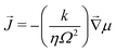 | (2) |
where k is the permeability, η is the viscosity of the solvent and Ω is the molar volume of the solvent. If the poroelastic substrate is a gel, note that the mobility k/(ηΩ2) can also be expressed in terms of the swelling ratio λ0 in the freely swollen state relative to the dry state as D/(![[scr N, script letter N]](https://www.rsc.org/images/entities/char_e52d.gif) aΩkBT)(λ03 − 1)/λ03 where a is the Avogadro number and D is the intrinsic diffusivity of the solvent molecules. The strain tensor ε is defined as:
aΩkBT)(λ03 − 1)/λ03 where a is the Avogadro number and D is the intrinsic diffusivity of the solvent molecules. The strain tensor ε is defined as:| | 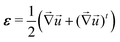 | (3) |
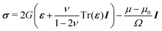
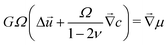
In the framework of linear poroelasticity, the stress tensor σ is given by:
| |  | (4) |
where
G is the shear modulus,
ν is the the Poisson ratio that characterizes the ability of a gel to absorb its solvent and
I is the identity tensor. We assume that the solvent and polymer molecules are incompressible and consequently the local volume variation is given by the local variation of the solvent concentration. This molecular incompressibility condition reads:
The mechanical equilibrium in the bulk of the poroelastic layer is described by the Navier equations:
| |  | (6) |
Combining the equations above we obtain
| |  | (7) |
where
| | 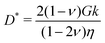 | (8) |
is an effective diffusion coefficient (also called the cooperative diffusion coefficient) and
Δ is the Laplace operator. Note that the material parameters
G,
k and thus
D* are effective parameters that depend on the initial state of the gel. In a nonlinear theory, they are also functions on the local deformation of the gel. Within the framework of linear poroelasticity however, we will assume that the deformed state is close enough to the initial state such that
G,
k and
D* can be treated as constant material parameters. Finally, combining
(3)–(6) and under the assumption that
c0 is homogeneous, we obtain
| |  | (9) |
2.2 Boundary conditions
At the free boundary, the gel is subjected to a force distribution ![[t with combining right harpoon above (vector)]](https://www.rsc.org/images/entities/i_char_0074_20d1.gif) and surface tension γs
and surface tension γs| | 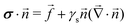 | (10) |
where ![[n with combining right harpoon above (vector)]](https://www.rsc.org/images/entities/i_char_006e_20d1.gif) and
and ![[f with combining right harpoon above (vector)]](https://www.rsc.org/images/entities/i_char_0066_20d1.gif) are the unit normal vector to the surface and traction forces exerted at the substrate boundary, respectively. γs is the surface tension of the solid. We are mostly interested in the case of an impermeable gel and thus
are the unit normal vector to the surface and traction forces exerted at the substrate boundary, respectively. γs is the surface tension of the solid. We are mostly interested in the case of an impermeable gel and thus| |  | (11) |
In addition, we assume that the substrate is infinitely thick and thus the displacement and stress fields vanish for z → −∞.
3 Deformation of a poroelastic half-space with surface tension
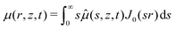
As mentioned in the introduction, we are interested in the response of a thick poroelastic substrate following the sudden application of a distribution of surface forces. For the sake of simplicity, and motivated by the specific question of elastowetting, we will focus here on axisymmetric force distribution only. With this choice of geometry, it is convenient to use cylindrico-polar coordinates (r,z) and restrict ourselves to time-dependent axisymmetric fields for the solvent concentration c(r,z,t), chemical potential μ(r,z,t) and displacement field (r,z,t):| | (r,z,t) = u(r,z,t)![[e with combining right harpoon above (vector)]](https://www.rsc.org/images/entities/i_char_0065_20d1.gif) r + v(r,z,t)z r + v(r,z,t)z | (12) |
Furthermore, we only consider in this paper the case where the traction force at the free boundary is purely normal, i.e. ∝ z. Although we will consider later time-dependent forcing, we first focus on the step response of the system i.e. when the surface force distribution is suddenly applied at t = 0 and subsequently maintained for t ≥ 0. We may therefore write = fz(r)H(t)z, where H(t) is the Heaviside step function. Thus, we have at the free surface:
| | 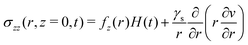 | (13) |
3.1 Hankel transform
In order to solve the equilibrium equations presented above, it is convenient to introduce the following Hankel transforms:| | 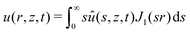 | (15) |
| |  | (16) |
| |  | (17) |
| |  | (18) |
where J0(z) and J1(z) are the zero and first order Bessel functions of the first kind, respectively.
3.2 Instantaneous deformation
When a traction force = fz(r)H(t)z is suddenly applied at the free surface at t = 0, the liquid has no time to migrate and the system first deforms instantaneously as an incompressible solid. This elastic deformation causes the chemical potential to drop below its equilibrium value μ0 and sets the fluid into motion. Using a superscript i to denote the instantaneous response, the instantaneous concentration field ci is thus ci = c0. As a consequence of the molecular incompressibility constraint (5) the instantaneous deformation field i satisfies  and thus Δμi = 0. From these two relations, it follows that each component of the displacement field ui and vi satisfies the biharmonic equation, i.e.: Δ2ui = Δ2vi = 0. The two fields are not independent and ui can be expressed in terms of vi using
  . Inserting the Hankel transforms into the biharmonic equation, we obtain a linear fourth-order ordinary differential equation for, say,
 ![[v with combining circumflex]](https://www.rsc.org/images/entities/i_char_0076_0302.gif) i:
i:| | 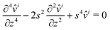 | (19) |
The above ordinary differential equation is readily solved and involves four unknown coefficients (that depend on s). Two of them are cancelled to satisfy  . The two remaining functions are found by making use of the two boundary conditions (13), (14) and we find:
| | 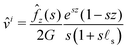 | (20) |
where
![[small script l]](https://www.rsc.org/images/entities/char_e146.gif) s
s =
γs/(2
G) is the elastocapillary length and
![[f with combining circumflex]](https://www.rsc.org/images/entities/i_char_0066_0302.gif) z
z(
s) is the Hankel transform of the surface traction
fz(
r). The radial component
ûi of the instantaneous displacement field is given by:
| | 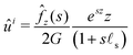 | (21) |
3.3 Final state
On a long-enough time scale, the system eventually reaches a thermodynamic equilibrium in which the solvent flux vanishes ( = ![[0 with combining right harpoon above (vector)]](https://www.rsc.org/images/entities/char_0030_20d1.gif) ) and the chemical potential relaxes to its equilibrium value μ0 (provided that the surface force vanishes for r → ∞). In this final stationary state (where quantities are denoted by superscript f), cf does not depend on time anymore and the concentration field therefore satisfies Δcf = 0. Note that, in contrast with the chemical potential which relaxes towards a homogeneous equilibrium value, the concentration field is heterogeneous in the final state if the force distribution at the free surface is not homogeneous. Because the concentration field is Laplacian and μf = μ0, the final displacement field f again satisfies a biharmonic equation Δ2uf = Δ2vf = 0 which again leads to an equation of the form (19) and whose solution is now:
) and the chemical potential relaxes to its equilibrium value μ0 (provided that the surface force vanishes for r → ∞). In this final stationary state (where quantities are denoted by superscript f), cf does not depend on time anymore and the concentration field therefore satisfies Δcf = 0. Note that, in contrast with the chemical potential which relaxes towards a homogeneous equilibrium value, the concentration field is heterogeneous in the final state if the force distribution at the free surface is not homogeneous. Because the concentration field is Laplacian and μf = μ0, the final displacement field f again satisfies a biharmonic equation Δ2uf = Δ2vf = 0 which again leads to an equation of the form (19) and whose solution is now:| | 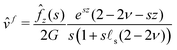 | (22) |
3.4 Time-dependent deformation
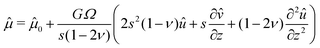
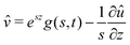
We now turn to the resolution of the time dependent problem. Although the time dependence only appears explicitly in the diffusion eqn (7), it cannot be solved independently because the boundary conditions involve c, μ and the displacement field . Using eqn (3)–(6), as well as the boundary conditions (13) and  , the fields ĉ, and
 ![[small mu, Greek, circumflex]](https://www.rsc.org/images/entities/i_char_e0b3.gif) can be expressed in terms of û:
can be expressed in terms of û:| | 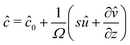 | (23) |
| |  | (24) |
| |  | (25) |
where the function g(s,t) is defined as:| | 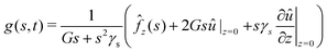 | (26) |
Plugging the above results in (7), we obtain the following non homogeneous fourth-order linear partial differential equation for û:
| | 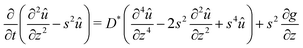 | (27) |
This equation is supplemented by the two boundary conditions (14) and (11) at the free surface while  . Furthermore, the initial condition is given by û(s,z,0) = ûi where ûi is defined by (21). Because we are interested for the first time in the step response of the system, this problem is best solved by introducing the Laplace transform Û(s,z,ω) of û(s,z,t) defined as:
| | 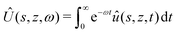 | (28) |
Plugging the above expression into the evolution eqn (27) for û(s,z,t) and making use of the initial condition û(s,z,0) = ûi, we now obtain a non-homogeneous fourth order linear ordinary differential equation that is easily solved by using the four boundary conditions mentioned previously.
3.5 Solution for a step forcing
We only write here the compact result for the (Hankel–Laplace transform of the) deflection Ẑ(s,ω) = Û(s, z = 0, ω) of the free surface:| | 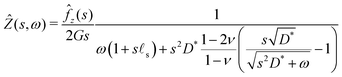 | (29) |
where we have used the result that the Laplace transform of the Heaviside step function H(t) is 1/ω. The inverse Hankel–Laplace transform can be obtained by the use of the inverse Hankel transform together with the help of the Bromwich integral that gives the inverse Laplace transform:| | 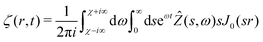 | (30) |
where χ is a real number such that the axis of integration ]χ − i∞,χ + i∞[, which is parallel to the imaginary axis, lies at the right of the pole of the integrand in (30), ensuring that the contour of integration is in the region of convergence. This solution is the step response of a poroelastic half-space subject to an arbitrary radially-symetric distribution of normal surface forces applied at t = 0 i.e. = fz(r)H(t)z. Let us first note that the two limiting cases described previously can be recovered using the initial and final value theorems:| | 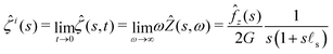 | (31) |
| |  | (32) |
The response of the gel is thus that of an incompressible solid at short time while it behaves as a compressible solid at long time. This apparent compressibility is due to the ability of the solvent to migrate and is quantified by the poroelastic Poisson ratio ν. When ν = 1/2, the gel cannot absorb or release any solvent and the final and initial states are identical. In that case, the inverse Laplace transform can be performed analytically and the deflection is ![[small xi, Greek, circumflex]](https://www.rsc.org/images/entities/i_char_e0b9.gif) (s,t) = i(s)H(t). This solution is the purely elastic response originally derived by Jerison and later by Style and Dufresnes. The displacement of the interface at large distances (small wavenumber s) behaves as ∼z(s)/(2Gs) and the deflection is thus damped by the bulk elasticity. At small distances (large s), the deflection behaves as ∼z(s)/(s2γs) and is thus dominated by surface tension. The crossover between the elastic and the capillary regime occurs at the scale of the elastocapillary length s.
(s,t) = i(s)H(t). This solution is the purely elastic response originally derived by Jerison and later by Style and Dufresnes. The displacement of the interface at large distances (small wavenumber s) behaves as ∼z(s)/(2Gs) and the deflection is thus damped by the bulk elasticity. At small distances (large s), the deflection behaves as ∼z(s)/(s2γs) and is thus dominated by surface tension. The crossover between the elastic and the capillary regime occurs at the scale of the elastocapillary length s.
3.6 General solution for arbitrary force distribution
The fundamental solution (30) derived above can be exploited to generate the impulsional response of the system to a forcing of the form = fz(r)δ(t)z (by taking the derivative) or convolved to generate the response to more general time-dependent forcing = fz(r)F(t)z. Indeed, using the Duhamel principle of superposition, the solution ξ(r,t) to this arbitrary time dependent forcing can be written in terms of the step response ζ(r,t) given in eqn (30):| |  | (33) |
This general solution will be investigated at the end of the next section but we first turn to the analysis of the solution (30) in the case of a hemispherical droplet on a poroelastic substrate (Fig. 1).
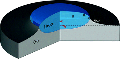 |
| | Fig. 1 Schematic representation of the problem and notations. A liquid hemispherical droplet with radius R and contact angle θ is deposited at time t = 0 at the surface of a poroelastic substrate. The black dashed line indicates the position of the free surface before the deposition of the liquid drop. Using cylindrico-polar coordinates (r,z) in the frame (r,z), the deflection of the free surface is given by the function ζ(r,t). | |
4 Results for hemispherical droplets
We now consider the specific case where the surface force distribution is due to a hemispherical droplet with radius R and contact angle θ. In this situation, the surface force distribution is  . The first term is due to the liquid/air surface tension that pulls on the substrate at the contact line while the second term is due to the Laplace pressure inside the spherical droplet that pushes the substrate. The zeroth-order Hankel transform of fz(r) is:
| | 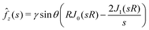 | (34) |
With this choice of surface force distribution, the interface profile ζ(r,t) is given by:
| | 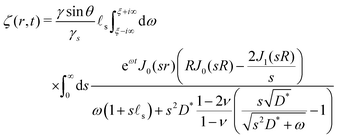 | (35) |
Let us note here that, in general, the wet and dry parts of the solid are likely to have different surface energies. However, taking this effect into account leads to a discontinuous boundary value problem that can be further transformed into coupled integral equations which cannot be solved analytically. This problem therefore remains, as mentioned in the introduction, an open question. Because we wish to focus this work on the effect of poroelasticity on elastowetting, we will assume here that the surface energies of the dry and wet parts of the solids are equal and given by γs. We now turn to the detailed analysis of eqn (35) for specific cases of broad physical interest.
4.1 Large drops
The first limiting case of interest is the case of large drops, i.e. R ≫ s. We plot in Fig. 2 the time evolution of the surface deformation for a large drop (R/s = 100), as well as the associated concentration and chemical potential fields. As seen in Fig. 2B the lower part of the drop sinks over time inside the soft substrate. The ridge height h(t) = ζ(R,t) on the other hand, increases in a non-trivial fashion after the initial deposition and its evolution is plotted in Fig. 2C. Before the deposition, the interface is flat h(0−) = 0. Right after the deposition, the height suddenly jumps to a height h(0+). Asymptotically, for large drops, the height h(0+) of the ridge is given by:| | 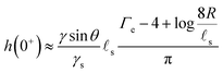 | (36) |
where Γe is the Euler–Mascheroni constant. Following this initial jump, the height of the ridge increases as the solvent migrates toward the ridge where the gel is under tension. At the same time, the ridge moves radially toward the interior of the drop up to a distance of s(γ![[thin space (1/6-em)]](https://www.rsc.org/images/entities/char_2009.gif) sinθ(1 − 2ν))/(4γs) in the final state. Because this time evolution is due to the diffusive migration of the solvent on a distance of order R, the stationary state is reached on a timescale of ∼R2/D*, as can be seen in the inset of Fig. 2C. Quite surprisingly for such a damped system, the ridge height first increases above its final stationary value h(∞) before relaxing toward h(∞) which is given asymptotically by:
sinθ(1 − 2ν))/(4γs) in the final state. Because this time evolution is due to the diffusive migration of the solvent on a distance of order R, the stationary state is reached on a timescale of ∼R2/D*, as can be seen in the inset of Fig. 2C. Quite surprisingly for such a damped system, the ridge height first increases above its final stationary value h(∞) before relaxing toward h(∞) which is given asymptotically by:| | 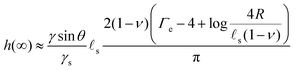 | (37) |
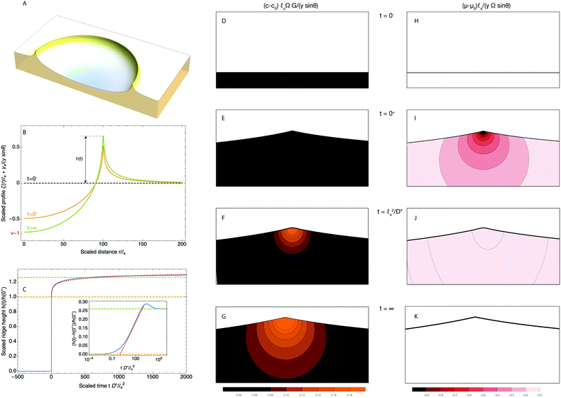 |
| | Fig. 2 Time dependent deformation of the poroelastic substrate following the deposition of a large drop (R/s = 100) and a poroelastic Poisson ratio of 3/10. (A) 3D view of a half space deformed by the drop showing the ridge at the triple line. The drop is not drawn for clarity. (B) Dimensionless profile of the interface ζ(r,t)/s at t = 0+ (orange curve) and t = ∞ (green curve). The initial position of the interface before deposition at t = 0− is indicated by a black dotted curve. (C) Time evolution of the height of the ridge (solid blue curve), scaled by its instantaneous value h(0+). The instantaneous response is indicated by an orange dashed line while the final equilibrium value is indicated by a green dashed line. The asymptotic law h(t) − h(0+) ∝ slog(tD*/s2) is shown by a red dotted curve. Shown in inset is the scaled poroelastic response (h(t) − h(0+))/h(0+) after deposition with a log scale for the time coordinate, clearly showing the overshoot behavior discussed in the text. (D–G) Evolution of the dimensionless solvent concentration field (c − c0)Ω before the deposition of the drop at t = 0− (D), right after deposition at t = 0+ (E), at t = s2/D* (F) and finally at t = ∞ (G). (H–K) Evolution of the dimensionless chemical potential field (μ − μ0)GΩ before the deposition of the drop at t = 0− (D), right after deposition at t = 0+ (E), at t = s2/D* (F) and finally at t = ∞ (G). In (D–K), the concentration and chemical potential fields are plotted in regions centered at R/s = 100 and have the width and height of 2s and s, respectively. | |
This non-trivial overshooting behavior can be understood by analyzing the two forces that are applied to the surface of the poroelastic substrate. While both forces imply migration of solvent over a lengthscale R, the Laplace pressure in the drop acts as a distributed pressure on the surface that pushes fluid only in the outward radial direction. On the other hand, the traction due to the air/liquid interface is a force localized at the triple line and draws fluid from both the inside and the outside of the drop. As a consequence the increase in height due to this traction relaxes twice as fast as the decrease in height due to the Laplace pressure. The combination of these two forces with slightly different timescales therefore produces the overshoot behavior seen in the inset of Fig. 2C.
Because the inverse Hankel–Laplace cannot be evaluated analytically, it is not possible to provide a simple expression (in the time domain) for the time evolution of the ridge height h(t). However, some crude approximations can be performed in order to gain further insight into the behavior of h(t). In the limit of large drop, we focus on the evolution of h(t) between the two intermediate timescales s2/D* ≪ t ≪ R2/D* and we will make the crude approximation that the evolution of h(t) in this regime is mostly due the evolution of the corresponding lengthscales 1/R ≪ s ≪ 1/s and we will check later that this approximation is self-consistent. In this limit, the Laplace transform of the increase of the ridge height h(t) − h(0+) is then approximately 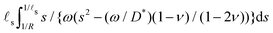 . This simpler expression can then be integrated along s and the resulting expression can finally be inverted in the time domain analytically to yield the scaling
| | | h(t) − h(0+) ∝ slog(tD*/s2) | (38) |
As seen in Fig. 2C, this expression fits rather well the numerical result between the two intermediate timescales s2/D* ≪ t ≪ R2/D*, as expected from our assumptions. Besides providing a reasonable approximation to the evolution of the ridge height, it also shows that the relevant timescale for the evolution of the ridge created by large drops is s2/D*. Beneath the drop, the depth of the valley is, at leading order, independent of the drop size and increases over time, from 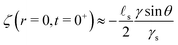 until it reaches
 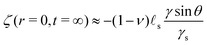 . As seen in Fig. 2B, the formula above are a good approximation for the case R/s = 100. Beneath the drop, the chemical potential increases right after the deposition. We find that, for large drops, the chemical potential beneath the drop at t = 0+ is given by:
| | 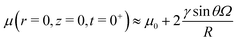 | (39) |
At the contact line however, the chemical potential diverges as log|r − R|. In the final state, the chemical potential relaxes everywhere to μ0. Similarly, the concentration of the solvent, initially equal to c0 reaches the following value beneath the drop in the steady state.
| | 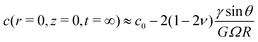 | (40) |
As can be seen from eqn (39) and (40), although the depth of the valley increases over time, the change in the concentration beneath the drop is very small. On the other hand, and while the change in the amplitude of the ridge is of the same order than that of the depth of the valley, the solvent concentration increases sharply (it also diverges as log|r − R|) beneath the ridge. We therefore only plot here the concentration (Fig. 2D–G) and chemical potential (Fig. 2H–K) fields in the vicinity of the contact line. As seen in those panels, the solvent concentration field (c − c0) is zero at t = 0+ but then increases sharply near the contact line where we also notice the radial (inward) displacement of the triple line over time.
4.2 Small drops
We now turn to the analysis of eqn (35) for a second case where analytical approximations are possible, namely, small drops (R ≪ s). We plot in Fig. 3B the evolution of the surface deformation at various times for small drops (R/s = 1/100). At the time of deposition, small drops adopt a lenticular shape and the substrate is flat outside of the drop. This is due to the fact that below the elasto-capillary length, all perturbations are damped by capillarity. Consequently, both the Laplace pressure and the surface tension at the contact line are balanced solely by the surface tension of the gel and not by its elasticity. As only surface tensions play a role in the force balance in this case, the situation is analogous to that of a liquid lens on a liquid bath, hence the lenticular shape. Indeed, beneath the drop, the depth of the valley is, at leading order, independent of time and is given by:| | 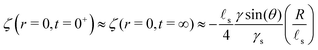 | (41) |
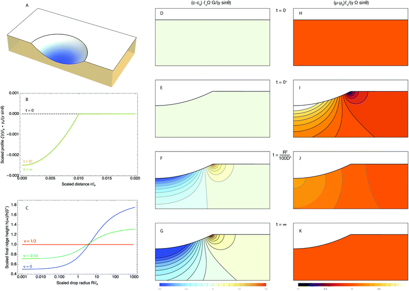 |
| | Fig. 3 Time dependent deformation of the poroelastic substrate following the deposition of a small drop (R/s = 1/100) and a poroelastic Poisson ratio of 3/10. (A) 3D view of a half space deformed by the drop showing the ridge at the triple line. The drop is not drawn for clarity. (B) Dimensionless profile of the interface ζ(r,t)/s at t = 0+ (orange curve) and t = ∞ (green curve). The initial position of the interface before deposition at t = 0− is indicated by a black dotted curve. To first order in R/s the shape of the deformed gel is unchanged. (C) Scaled value of the final ridge height h(∞)/h(0+) as a function of the scale radius of the drop R/s for three different values of the poroelastic Poisson ratio (ν = 1/2: red curve, ν = 3/10: green curve, ν = 0: blue curve). (D–G) Evolution of the dimensionless solvent concentration field (c − c0)sΩG/(γsinθ) before the deposition of the drop at t = 0− (D), right after deposition at t = 0+ (E), at t = R2/10D* (F) and finally at t = ∞ (G). (H–K) Evolution of the dimensionless chemical potential field (μ − μ0)s/(γΩsinθ) before the deposition of the drop at t = 0− (D), right after deposition at t = 0+ (E), at t = R2/10D* (F) and finally at t = ∞ (G). In (D–K), the concentration and chemical potential fields are plotted in regions centered at R/s = 1/100 and have the width and height of 2R and R, respectively. | |
As the consequence of the lenticular shape, we therefore expect the ridge height to be asymptotically zero at leading order. Right after the deposition, the height suddenly jumps to a small height h(0+) which, for small drops is given by the first non-zero term of an expansion in R/s:
| |  | (42) |
After relaxation, the ridge height reaches h(∞) which is given asymptotically by:
| |  | (43) |
We note that the ridge height is now quadratic in R/s. The consequence of this is that, at first order in R/s, and in stark contrast with large drops, the profile is flat outside the drop. To the same order the profile is thus independent of time for small drops, as can be seen in Fig. 3B. This effect could in fact be expected since the shape of the substrate deformation is controlled solely by capillarity for small drops. As it is therefore independent of the mechanical properties of the substrate (again, to first order in R/s), the profile is both independent of the shear modulus and the poroelastic Poisson ratio, i.e. of the ability of the substrate to reorganize the solvent. We note that, in contrast with large drops, the ratio h(∞)/h(0+) is smaller than 1 and thus small drops gradually sink inside the gel although this is a second order effect on R/s. This can also be seen in Fig. 3C that shows the ratio h(∞)/h(0+) as a function of the drop size R ≪ s for different values of the poroelastic ratio ν. We can also note from this panel that the transition from the symmetric ridge of large drops to the tilted ridge of small drops is quite broad and occurs over several decades of the ratio R/s. This result is quite similar to the transition observed in purely elastic systems that we investigated previously.24 Furthermore, note that since R ≪ s, the relevant timescale for the evolution of the ridge profile is not s2/D* anymore, as was the case for large drops, but R2/D*. Now if the shape of the substrate is, at leading order, independent of time, how does the solvent evolve? Beneath the drop, the chemical potential increases right after the deposition while it drops under the ridge. Asymptotically, we find that the chemical potential beneath the drop is given by:
| |  | (44) |
As the chemical potential converges to μ0 away from the drop, there is indeed a gradient of chemical potential that drives fluid motion. In the final state, the concentration of the solvent beneath the drop is given by:
| |  | (45) |
The corresponding concentration and chemical potential are plotted in Fig. 3D–G and H–K, respectively.
4.3 Drop removal
We now investigate the effect of removing the drop at the free surface after a residence time τres. We therefore now have a forcing of the form = {fz(r)H(t) − fz(r)H(t − τres)}z. Using the convolution integral given in eqn (35), the solution ζres(r,t) describing the profile of the interface for the deposition/removal problem is simply given by:| | | ζres(r,t) = ζ(r,t) − H(t − τres)ζ(r,t − τres) | (46) |
where ζ(r,t) is given by (35). As the ridge is pronounced only for R ≫ s, we focus here on large drops only. We plot in Fig. 4A the profile of the poroelastic substrate for a residence time τres = 10s2/D* at various times following the removal of the drop. These curves indicate that the drop leaves a footprint on the gel that slowly relaxes to a flat interface. More quantitatively, and as seen in Fig. 4, the height of the ridge drops by an amount h(0+) immediately following the removal of the drop, at time τres+, i.e. h(τres+) = h(τres−) − h(0+). Following this instantaneous elastic response, the height then relaxes toward zero as the solvent diffuses back to its original concentration c = c0: this is the poroelastic response. We plot in the inset of Fig. 4B the relaxation of the ridge for several values of the residence time τres. As seen in Fig. 4C, the relaxation depends on the history of the gel and is faster for smaller residence time τres. For residence time τres smaller than the timescale s2/D* the ridge height decreases as ∼1/t at intermediate timescales s2/D* ≪ t ≪ R2/D*. However, for residence time τres larger than the timescale s2/D*, the ridge height decreases more slowly, as ∼−log(t). In order to estimate the lifetime of the drop footprint, we define a time τlife which corresponds to the time it takes for the deformation to reach a critical thickness hc, i.e. we defined τlife as the solution of the equation:
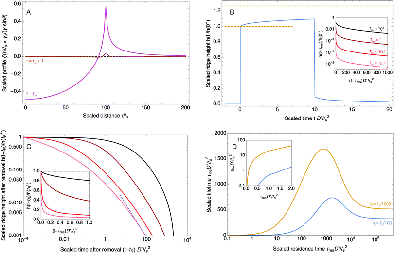 |
| | Fig. 4 Time dependent deformation of the poroelastic substrate following the removal of a large drop (R/s = 100) and a poroelastic Poisson ratio of 3/10. (A) Profile of the interface at t = τres− (magenta curve) and t = τres + s2/D* (brown curve). The initial position of the interface before deposition at t = 0− is indicated by a black dotted curve. (B) Time evolution of the height of the ridge (solid blue curve), scaled by its instantaneous response at the time of deposition h(0+). The instantaneous response is indicated by an orange dashed line while the final equilibrium value is indicated by a green dashed line. The drop is removed at t = τres = 10s2/D*. The height of the ridge first elastically decreases instantaneously by an amount of h(0+) before relaxing poroelastically. Several scaled h(t − τres)/h(0+) profiles of the poroelastic relaxation are shown in the inset for different values of the residence time t = τres. The residence times are given in units of D*/s2. (C) log–log plots of the scaled poroelastic profiles h(t − τres)/h(τres+) as a function of the scaled time after removal (t − τres)D*/s2 for different values of the residence time. A close view in linear scale is given in the inset. (D) Scaled lifetime of the footprint of the drop τlifeD*/s2 as a function of the scaled residence time of the drop τresD*/s2 for two different values of the critical thickness hc below which the footprint disappears. | |
In the present study, the value of this critical thickness is of course arbitrary but it can be quantified for specific applications. In the context of wetting for example, surface defects as small as 10 nm can pin the contact line and affect the static equilibrium angle. As a consequence, if the footprint of a drop is thicker than this critical thickness, it will have consequences at the macroscopic scale on the wetting properties of the gel for instance. As seen in Fig. 4D, the lifetime of the drop footprint strongly depends on this critical thickness and shows a non-trivial dependence on the residence time τres of the drop. We first note that the residence time must be larger than a critical value for the height of the footprint to be larger than hc. This effect can be seen in the inset of Fig. 4D. Above this critical residence time, the footprint lifetime τlife first increases with the residence time τres until the residence time becomes comparable with the equilibrium time R2/D*. After this value, the lifetime decreases. This decrease is simply the consequence of the overshoot effect described previously for the growth of the ridge. When the residence time is much larger than R2/D*, then the gel has reached its equilibrium before the drop is removed. In that case, the lifetime of the footprint does not depend on the residence time of the drop and therefore τlife saturates to a finite value.
5 Discussion
In typical experiments of elastowetting, s is typically of the order of a few microns but can be as large as a millimeter thanks to recent advances in polymer technologies.49,50 The effective diffusion coefficient D* is typically in the range 10−11–10−10 m2 s−1 depending on the swelling ratio and the length of the free chains51,52 while values in the range 0.2–0.4 are reported for the poroelastic Poisson ratio.53–55 For such orders of magnitude of the physical parameters, the deformation created by a 1 mm droplet will take as long as ∼105 s to reach its equlibrium state. More quantitatively, for an elastocapillary length of 10 μm, a 1 mm drop with a residence time of 20 s will leave a footprint thicker than 100 nm for also roughly 20 s and it will leave a footprint thicker than 10 nm for more than 7 minutes. Similarly, a drop resting on a poroelastic substrate for 10 minutes will leave a circular footprint thicker than 10 nm for more than 2 hours. Preliminary experiments performed with water droplets on thick PDMS layers are in qualitative agreement, as seen in Fig. 5, with our predictions. A more quantitative experimental study is currently being performed by our group and is beyond the scope of the present article. Because nanometer-scale defects can pin a contact line, we expect that the residence time of the drop on the deformable substrate will have a dramatic impact on the measurement of the fundamental material properties of considerable practical interest, such as its surface tension or contact angle hysteresis. Those footprints will also affect drop spreading. In addition, because nanoscale surface features are strong enough to affect the polarity and the migration of living cells,56–59 we expect that the new theoretical developments presented in this paper will be important to finely model the locomotion of cells in living tissues and on soft materials.
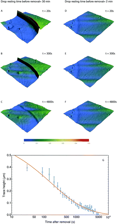 |
| | Fig. 5 Relaxation of the ridge under the contact line following the removal of the drop for a resting time of 30 minutes (A–C) and 2 minutes (D–F). In both cases 5 μL water droplets were placed on a freshly prepared thick PDMS substrate (thickness 1358 μm, shear modulus 1.2 kPa) and a region of ∼750 × 750 μm2 was scanned at regular intervals using a 3D profiler (Microsurf 3D, Fogal Nanotech, France) with a lateral resolution of 1.89 μm and a vertical resolution of 50 nm. The first scan was acquired roughly for 20 s following the removal of the drops. The color-coded heights are in microns. As seen in (D–F), no trace could be detected for a residence time of 2 minutes. For a residence time of 30 minutes on the other hand (A–C), the footprint of the drop is initially around 0.5 μm and is still around 100 nm after 4800 s. (G) Time evolution of the height of the trace following drop removal (same parameters as in A–C). The blue circles are the experimental data and the solid orange curve is the theoretical prediction given by eqn (46). For the theoretical curve, the droplet radius and substrate stiffness were taken from the experiment while the surface tension was taken as γs = 40 mN m−1 and the poroelastic Poisson ratio was taken as ν = 0.3. The effective diffusion coefficient D* was found by fitting the data with the model. The best fit for D* was found to be ∼ 2 × 10⁻¹¹ m2 s−1, in good agreement with other values found in the literature. | |
In our study, we have also seen that another consequence of merging the linear poroelastic theory with the elastowetting problem introduces a new divergence: the solvent concentration diverges as ∼log|r − R| near the contact line. While several approaches might be able to regularize this divergence, for example by taking into account the finite thickness of the gel, the material and geometrical nonlinearities or through the introduction of a finite width for the contact line, the existence of this divergence suggests that extreme phenomena such as phase separation, fracture or instabilities could occur at the contact line.60,61 Indeed, the coexistence of multiple phases at the contact line has been recently reported in indentation experiments.22 Further work, for example based on nonlinear poroelastic theory, will be needed in order to shed light on the behavior of gels near contact lines.
In a different line of thought, the wetting of saturated gels by drops of their own solvent opens interesting questions. Because the presence of a drop changes the chemical potential away from the drop, several drops may interact with each other by mass exchange throughout the gel. For thick gels (when the thickness of the gel is much larger than s and R), the chemical potential increases above its reference value away from the drop and will tend to suck fluid inside the gel. Because large drops will create a stronger change in the chemical potential than small drops we thus expect large drops to grow at the expense of smaller droplets. For thinner gels however, the effect of finite depth is likely to form a dimple within which the chemical potential drops below its reference value, and thus promotes the growth of smaller droplets nearby. Although speculative, this possibility might open a new route to new original methods to control droplet nucleation and dew collection on soft materials.
Conflicts of interest
There are no conflicts of interest to declare.
Acknowledgements
ANR (Agence Nationale de la Recherche) and CGI (Commisariat à l'Investissement d'Avenir) are gratefully acknowledged for their financial support through the GELWET project (ANR-17-CE30-0016), the Labex SEAM (Science and Engineering for Advanced Materials and devices - ANR 11 LABX 086, ANR 11 IDEX 05 02) and through the funding of the POLYWET project.
References
- M. Sokuler,
et al., The softer the better: Fast condensation on soft surfaces, Langmuir, 2010, 26, 1544–1547 CrossRef CAS PubMed.
- M. A. Unger, H.-P. Chou, T. Thorsen, A. Scherer and S. R. Quake, Monolithic Microfabricated Valves and Pumps by Multilayer Soft Lithography, Science, 2000, 288, 113–116 CrossRef CAS PubMed.
- T. Boland, T. Xu, B. Damon and X. Cui, Application of inkjet printing to tissue engineering, Biotechnol. J., 2006, 1, 910–917 CrossRef CAS PubMed.
- S. Chung,
et al., Inkjet-printed stretchable silver electrode on wave structured elastomeric substrate, Appl. Phys. Lett., 2011, 98, 2011–2014 Search PubMed.
- G. R. Lester, Contact angles of liquids at deformable solid surfaces, J. Colloid Sci., 1961, 16, 315–326 CrossRef CAS.
- G. R. Lester, Contact angles of liquids on organic solids, Nature, 1966, 209, 1126–1227 CrossRef CAS.
- M. E. R. Shanahan, Contact Angle Equilibrium on Thin Elastic Solids, J. Adhes., 1985, 18, 247–267 CrossRef CAS.
- M. E. R. Shanahan and P. G. de Gennes, L'arête produite par un coin liquide près de la ligne triple de contact solide/liquide/fluide, C. R. Acad. Sci. Paris, 1986, 302, 517–521 Search PubMed.
- M. E. R. Shanahan, The influence of solid micro-deformation on contact angle equilibrium, J. Phys. D, 1987, 20, 945–950 CrossRef CAS.
- D. Long, A. Ajdari and L. Leibler, Static and dynamic wetting properties of thin rubber films, Langmuir, 1996, 12, 5221–5230 CrossRef CAS.
- Y.-S. Yu, Z. Yang and Y.-P. Zhao, Role of vertical component of surface tension of the droplet on the elastic deformation of PDMS membrane, J. Adhes. Sci. Technol., 2008, 22, 687–698 CAS.
- Y. S. Yu and Y. P. Zhao, Elastic deformation of soft membrane with finite thickness induced by a sessile liquid droplet, J. Colloid Interface Sci., 2009, 339, 489–494 CrossRef CAS PubMed.
- R. Pericet-Camara,
et al., Solid-supported thin elastomer films deformed by microdrops, Soft Matter, 2009, 5, 3611–3617 RSC.
- B. Roman and J. Bico, Elasto-capillarity: deforming an elastic structure with a liquid droplet, J. Phys.: Condens. Matter, 2010, 22, 493101 CrossRef CAS PubMed.
- L. Limat, Straight contact lines on a soft, incompressible solid, Eur. Phys. J. E: Soft Matter Biol. Phys., 2012, 35, 134–147 CrossRef CAS PubMed.
- R. W. Style and E. R. Dufresne, Static wetting on deformable substrates, from liquids to soft solids, Soft Matter, 2012, 8, 7177 RSC.
- R. W. Style,
et al., Universal deformation of soft substrates near a contact line and the direct measure- ment of solid surface stresses, Phys. Rev. Lett., 2013, 066103 Search PubMed.
- R. W. Style, C. Hyland, R. Boltyanskiy, J. S. Wettlaufer and E. R. Dufresne, Surface tension and contact with soft elastic solids, Nat. Commun., 2013, 4, 2728 Search PubMed.
- S. Karpitschka,
et al., Droplets move over viscoelastic substrates by surfing a ridge, Nat. Commun., 2015, 6, 7891 CrossRef CAS PubMed.
- R. W. Style,
et al., Patterning droplets with durotaxis, Proc. Natl. Acad. Sci. U. S. A., 2013, 110, 12541–12544 CrossRef CAS PubMed.
- S. J. Park,
et al., Visualization of asymmetric wetting ridges on soft solids with X-ray microscopy, Nat. Commun., 2014, 5, 4369 CAS.
- K. E. Jensen, R. Sarfati, R. W. Style, R. Boltyanskiy, A. Chakrabarti, M. K. Chaudhury and E. R. Dufresne, Wetting and phase separation in soft adhesion, Proc. Natl. Acad. Sci. U. S. A., 2015, 112, 14490–14494 CrossRef CAS PubMed.
-
M. Zhao, et al., Thickness effects in the wetting of soft solids, 2017, under review.
- J. Dervaux and L. Limat, Contact lines on soft solids with uniform surface tension: analytical solutions and double transition for increasing deformability, Proc. R. Soc. A, 2015, 471, 20140813 CrossRef.
-
R. De Pascalis, J. Dervaux, I. Ionescu and L. Limat, Nonlinear elastowetting: multiscale modeling of the triple line, under review.
- W. Hong, X. Zhao, J. Zhou and Z. Suo, J. Mech. Phys. Solids, 2008, 56, 1779–1793 CrossRef CAS.
- W. Hong, Z. Liu and Z. Suo, Int. J. Solids Struct., 2009, 46, 3282–3289 CrossRef CAS.
- C. Y. Hui and V. Muralidharan, J. Chem. Phys., 2005, 123, 154905 CrossRef PubMed.
- Y. Hu and Z. Suo, Viscoelasticity and poroelasticity in elastomeric gels, Acta Mech. Solida Sin., 2012, 25, 441–458 CrossRef.
- J. R. Rice and M. P. Cleary, Some basic stress diffusion solutions for fluid-saturated elastic porous media with compressible constituents, Rev. Geophys. Space Phys., 1976, 14, 227–241 CrossRef.
-
H. F. Wang, Theory of Linear Poroelasticity with Applications to Geomechanics and Hydrogeology, Princeton University Press, 2000 Search PubMed.
- M. A. Biot, J. Appl. Phys., 1941, 12, 155–164 CrossRef.
- J. J. Roberts, A. Earnshaw, V. L. Ferguson and S. J. Bryant, Comparative study of the viscoelastic mechanical behavior of agarose and poly(ethylene glycol) hydrogels, J. Biomed. Mater. Res., Part B, 2011, 99, 158–169 CrossRef PubMed.
- Y. Liu and M. B. Chan-Park, Hydrogel based on interpenetrating polymer networks of dextran and gelatin for vascular tissue engineering, Biomaterials, 2009, 30, 196–207 CrossRef PubMed.
- Xuanhe Jeong-Yun Sun, Widusha R.K. Zhao, Kyu Hwan Illeperuma, David J. Oh and Joost J. Mooney, Vlassak, Zhigang Suo. Highly stretchable and tough hydrogels, Nature, 2012, 489(7414), 133–136 CrossRef PubMed.
-
J. D. Ferry, Viscoelastic Properties of Polymers, John Wiley & Sons, Inc., New York, 1980 Search PubMed.
- X. Zhao, N. Huebsch and D. J. Mooney,
et al., Stress-relaxation behavior in gels with ionic and covalent crosslinks, J. Appl. Phys., 2010, 107, 063509 CrossRef PubMed.
- D. T. Chen, Q. Wen and P. A. Janmey,
et al., Rheology of soft materials, Annu. Rev. Condens. Matter Phys., 2010, 1, 301–322 CrossRef CAS.
- Y. Hu, X. Chen and G. M. Whitesides,
et al., Indentation of poly- dimethylsiloxane submerged in organic solvents, J. Mater. Res., 2011, 26, 785–795 CrossRef CAS.
- Z. I. Kalcioglu, R. Mahmoodian and Y. Hu,
et al., From macro- to microscale poroelastic characterization of polymeric hydrogels via indentation, Soft Matter, 2012, 8, 3393–3398 RSC.
- D. G. Strange, T. L. Fletcher and K. Tonsomboon,
et al., Separating poroviscoelastic deformation mechanisms in hydrogels, Appl. Phys. Lett., 2013, 102, 031913 CrossRef.
- L. L. Hyland, M. B. Taraban and Y. Feng,
et al., Viscoelastic properties and nanoscale structures of composite oligopeptide- polysaccharide hydrogels, Biopolymers, 2012, 97, 177–188 CrossRef CAS PubMed.
- J. E. Olberding and J. Francis Suh, A dual optimization method for the material parameter identification of a biphasic poro- viscoelastic hydrogel: Potential application to hypercompliant soft tissues, J. Biomech., 2006, 39, 2468–2475 CrossRef PubMed.
- X. Wang and W. Hong, A visco-poroelastic theory for polymeric gels, Proc. R. Soc. A, 2012, 468, 3824–3841 CrossRef.
- M. Biot, Theory of deformation of a porous viscoelastic anisotropic solid, J. Appl. Phys., 1956, 27, 459–467 CrossRef.
- Y. Weitsman, Stress assisted diffusion in elastic and viscoelastic materials, J. Mech. Phys. Solids, 1987, 35, 73–94 CrossRef.
- Y. Weitsman, A continuum diffusion model for viscoelastic materials, J. Phys. Chem., 1990, 94, 961–968 CrossRef CAS.
- S. Karpitschka, S. Das, M. van Gorcum, H. Perrin, B. Andreotti and J. H. Snoeijer, Droplets move over viscoelastic substrates by surfing a ridge, Nat. Commun., 2015, 6, 7891 CrossRef CAS PubMed.
- R. N. Palchesko, L. Zhang, Y. Sun and A. W. Feinberg, PLoS One, 2012, 7, e51499 CAS.
- T. Narita, K. Mayumi, G. Ducouret and P. Hébraud, Macromolecules, 2013, 46, 4174 CrossRef CAS.
- J. Yoon, S. Cai, Z. Suo and R. C. Hayward, Poroelastic swelling kinetics of thin hydrogel layers: comparison of theory and experiment, Soft Matter, 2010, 6(23), 6004 RSC.
- S. Matsukawa and I. Ando, A Study of Self-Diffusion of Molecules in Polymer Gel byPulsed-Gradient Spin-Echo 1H NMR, Macromolecules, 1996, 29, 7136–7140 CrossRef CAS.
- S. Hirotsu, J. Chem. Phys., 1991, 94, 3949 CrossRef CAS.
- C. Li, Z. Hu and Y. Li, Phys. Rev. E: Stat. Phys., Plasmas, Fluids, Relat. Interdiscip. Top., 1993, 48, 603 CrossRef CAS.
- K. Urayama, T. Takigawa and T. Masuda, Poisson's ratio of poly(vinyl alcohol) gels, Macromolecules, 1993, 26(12), 3092–3096 CrossRef CAS.
- M. J. Dalby, M. O. Riehle, S. J. Yarwood, C. D. Wilkinson and A. S. Curtis, Nucleus alignment and cell signaling in fibroblasts: response to a micro-grooved topography, Exp. Cell Res., 2003, 284, 274–282 CrossRef CAS PubMed.
- K. A. Diehl, J. D. Foley, P. F. Nealey and C. J. Murphy, Nanoscale topography modulates corneal epithelial cell migration, J. Biomed. Mater. Res., Part A, 2005, 75(3), 603–611 CrossRef CAS PubMed.
- J. P. Kaiser, A. Reinmann and A. Bruinink, The effect of topographic characteristics on cell migration velocity, Biomaterials, 2006, 27, 5230–5241 CrossRef CAS PubMed.
- J. Park,
et al., Directed migration of cancer cells guided by the graded texture of the underlying matrix, Nat. Mater., 2016, 15(7), 792–801 CrossRef CAS PubMed.
- J. Dervaux, Y. Couder, M. A. Guedeau-Boudeville and M. Ben Amar, Shape transition in artificial tumors: from smooth buckles to singular creases, Phys. Rev. Lett., 2011, 107, 018103 CrossRef PubMed.
- J. Dervaux and M. Ben Amar, Mechanical Instabilities of gels, Annu. Rev. Condens. Matter Phys., 2012, 3, 311–332 CrossRef CAS.
|
| This journal is © The Royal Society of Chemistry 2018 |

 a,
Laurent
Limat
a and
Julien
Dervaux
a,
Laurent
Limat
a and
Julien
Dervaux


 and thus Δμi = 0. From these two relations, it follows that each component of the displacement field ui and vi satisfies the biharmonic equation, i.e.: Δ2ui = Δ2vi = 0. The two fields are not independent and ui can be expressed in terms of vi using
  . Inserting the Hankel transforms into the biharmonic equation, we obtain a linear fourth-order ordinary differential equation for, say,
 . The two remaining functions are found by making use of the two boundary conditions (13), (14) and we find:


 , the fields ĉ,


 . Furthermore, the initial condition is given by û(s,z,0) = ûi where ûi is defined by (21). Because we are interested for the first time in the step response of the system, this problem is best solved by introducing the Laplace transform Û(s,z,ω) of û(s,z,t) defined as:


 . The first term is due to the liquid/air surface tension that pulls on the substrate at the contact line while the second term is due to the Laplace pressure inside the spherical droplet that pushes the substrate. The zeroth-order Hankel transform of fz(r) is:


 . This simpler expression can then be integrated along s and the resulting expression can finally be inverted in the time domain analytically to yield the scaling
 until it reaches
  . As seen in Fig. 2B, the formula above are a good approximation for the case R/


