
Self-assembly of cubic colloidal particles at fluid–fluid interfaces by hexapolar capillary interactions†
Giuseppe
Soligno
 *a,
Marjolein
Dijkstra
b and
René
van Roij
a
*a,
Marjolein
Dijkstra
b and
René
van Roij
a
aInstitute for Theoretical Physics, Center for Extreme Matter and Emergent Phenomena, Utrecht University, Princetonplein 5, 3584 CC Utrecht, The Netherlands. E-mail: g.soligno@uu.nl
bSoft Condensed Matter, Debye Institute for Nanomaterials Science, Department of Physics, Utrecht University, Princetonplein 1, Utrecht 3584 CC, The Netherlands
First published on 3rd November 2017
Abstract
Colloidal particles adsorbed at fluid–fluid interfaces can self-assemble, thanks to capillary interactions, into 2D ordered structures. Recently, it has been predicted by theoretical and numerical calculations [G. Soligno et al., Phys. Rev. Lett., 2016, 116, 258001] that cubes with smooth edges adsorbed at a flat fluid–fluid interface generate hexapolar capillary deformations that cause the particles to self-assemble into honeycomb and hexagonal lattices, at equilibrium and for Young's contact angle π/2. Here we extend these results. Firstly, we show that capillary interactions induced by hexapolar deformations can drive the particles at the interface to form also thermodynamically-stable square lattices, in addition to honeycomb and hexagonal lattices. Then, we study the effects of tuning the particle shape on the particle self-assembly at the interface, considering, respectively, smooth-edge cubes, sharp-edge cubes, slightly truncated-edge cubes, and highly truncated-edge cubes. In our calculations, both capillary and hard-particle interactions are taken into account. We show that such variations in the particle shape significantly affect both qualitatively and quantitatively the self-assembly of the particles at the interface, and we sum up our results in the form of temperature–density phase diagrams. For example, using typical experimental parameters, our results show that only 4-to-5 nm sized sharp-edge and smooth-edge cubes can self-assemble into a honeycomb lattice, while slightly and highly truncated-edge cubes can form a honeycomb lattice only if they have a 8-to-12 and 10-to-16 nm size, respectively, for the same experimental parameters. Also, our results show that the capillarity-induced square lattice phase is stable only for the smooth-edge and truncated-edge cubes, but not for the sharp-edge cubes.
I. Introduction
Colloidal particles strongly adsorb at fluid–fluid interfaces,1,2 allowing the formation of stable particle monolayers at the interface. Since a pioneering study by Pieranski,3 great interest has been devoted to these quasi-2D particle systems,4–6 which have many important applications, for example in coatings7–9 and for the stabilization of emulsions.10–18 Because of Young's Law, an adsorbed colloidal particle can generate capillary deformations in the fluid–fluid interface shape, which depend on the particle shape and surface chemistry,19–26 and on the bare curvature of the fluid–fluid interface.27–33 Such deformations induce capillary interactions between the adsorbed particles34,35 that can be exploited to regulate the self-assembly of the particles while confined to the fluid–fluid interface,36–43 providing a route to build 2D ordered structures.For example, the realization of a honeycomb (graphene-like) lattice with a period of a few nanometers would be extremely important for the semiconductor properties that such a material would have.44–46 Recent experiments47–49 have shown that cubic nanocrystals (of roughly 5-to-10 nm size) adsorbed at fluid–fluid interfaces can self-assemble into atomically-coherent honeycomb structures, although the underlying mechanism is still under investigation. While in ref. 47–49 the self-assembly is justified using only van der Waals forces and the steric interactions due to capping ligands, thereby ignoring capillary interactions, we suggested recently on the basis of theoretical and numerical calculations50 that capillarity is likely to be the driving force for the observed structures.
In ref. 50 we showed that cubic colloidal particles with smooth edges adsorbed at a fluid–fluid interface generate hexapolar capillary deformations in the interface height profile, when Young's contact angle θ is such that |cos![[thin space (1/6-em)]](https://www.rsc.org/images/entities/char_2009.gif) θ| ≤ 0.2. Thanks to the capillary interactions induced by such hexapoles, the cubes can self-assemble at the fluid–fluid interface into thermodynamically-stable honeycomb and hexagonal lattices. In this work, to further understand the experiments in ref. 47–49 where nanocubes with edges truncated at different levels are used,51 we investigate the effects of tuning the shape of the cubic particles. We consider four particle shapes, shown in Fig. 1 and defined in Appendix A: standard (i.e. sharp-edge) cubes, smooth-edge cubes (like the ones considered in ref. 50), slightly truncated-edge cubes, and highly truncated-edge cubes. We show that, for a Young's contact angle θ = π/2, adsorbed particles with any of these shapes induce a hexapolar deformation in the fluid–fluid interface height profile. However, two major factors are affected by varying the particle shape: the magnitude of the hexapolar capillary deformations and the center-to-center contact distances between the particles in the self-assembled lattices at the interface. This, we show, significantly affects both qualitatively and quantitatively the capillary interactions and the self-assembly of the particles at the interface. In addition, in this paper we prove that the hexapole-generating particles adsorbed at the interface can self-assemble, by capillary interactions, also in thermodynamically-stable square lattices, while in ref. 50 only hexagonal and honeycomb lattices were considered.
θ| ≤ 0.2. Thanks to the capillary interactions induced by such hexapoles, the cubes can self-assemble at the fluid–fluid interface into thermodynamically-stable honeycomb and hexagonal lattices. In this work, to further understand the experiments in ref. 47–49 where nanocubes with edges truncated at different levels are used,51 we investigate the effects of tuning the shape of the cubic particles. We consider four particle shapes, shown in Fig. 1 and defined in Appendix A: standard (i.e. sharp-edge) cubes, smooth-edge cubes (like the ones considered in ref. 50), slightly truncated-edge cubes, and highly truncated-edge cubes. We show that, for a Young's contact angle θ = π/2, adsorbed particles with any of these shapes induce a hexapolar deformation in the fluid–fluid interface height profile. However, two major factors are affected by varying the particle shape: the magnitude of the hexapolar capillary deformations and the center-to-center contact distances between the particles in the self-assembled lattices at the interface. This, we show, significantly affects both qualitatively and quantitatively the capillary interactions and the self-assembly of the particles at the interface. In addition, in this paper we prove that the hexapole-generating particles adsorbed at the interface can self-assemble, by capillary interactions, also in thermodynamically-stable square lattices, while in ref. 50 only hexagonal and honeycomb lattices were considered.
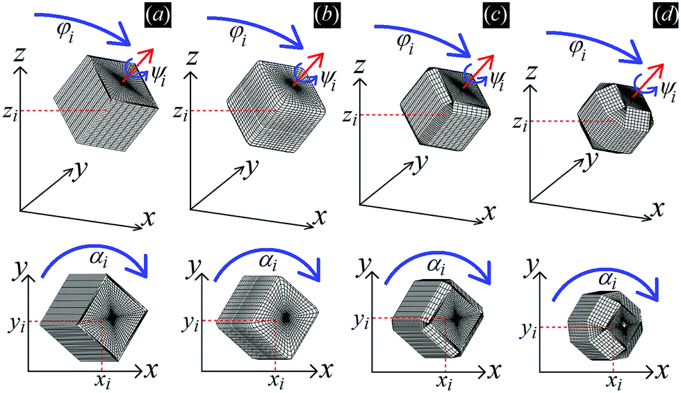 | ||
| Fig. 1 Sketch of the configuration (xi,yi,zi,φi,ψi,αi) of the generic i-th particle adsorbed at the fluid–fluid interface, with i = 1,…N and N the total number of adsorbed particles, using as particle shape (a) a sharp-edge cube, (b) a smooth-edge cube, (c) a slightly truncated-edge cube, and (d) a highly truncated-edge cube, respectively. The i-th particle has center of mass with Cartesian coordinates xi, yi, zi, an angle φi between its vertical axis and the z axis, an internal Euler angle ψi around its vertical axis, and an azimuthal orientation αi in the z = 0 plane. The plane z = 0 corresponds to the flat fluid–fluid interface when no particle is adsorbed. The particle vertical axis is sketched with a red arrow in the figures. Note that φ = 0 when the cube has two of its six faces parallel to the plane z = 0, and ψ = 0 when the cube has, for any given φ, at least six of its twelve sides parallel to the plane z = 0. | ||
Interestingly, all the three lattices predicted here (honeycomb, hexagonal, square) are observed in ref. 47–49 by the nanocubes at the interface. It is important to note that the orientation of each single nanocube at the interface – with one cube vertex upwards with respect to the interface plane – in the experimentally observed honeycomb and hexagonal lattices matches with our theoretical predictions. However, the nanocubes in the square lattice are found lying flat at the interface in the experiments, while we predict a vertex-up configuration in the square lattice as well. In addition, linear aggregates of adsorbed nanocubes – in principle compatible with either a hexagonal or a square lattice – are also observed in the experiments of ref. 47, but the claimed orientation at the interface of the nanocubes in these linear structures is with one edge up, and not the vertex-up configuration as we predict. Therefore, further investigation is still required to fully understand the systems in ref. 47–49. We point out that in this paper we consider (mainly for length reasons) only the case θ = π/2, i.e. the cubes have the same wettability with the two fluids forming the interface. If instead the cubes prefer to be wet by one of the two fluids, then capillary effects may be highly affected. In addition, van der Waals interactions between the adsorbed nanocubes may become relevant, compared to capillary effects, when the particles are (almost) at their contact distance, see Appendix B. Therefore, while the long-range ordered arrangement of the nanocube lattices found in ref. 47–49 is likely driven by capillarity, the precise final orientation of each single nanocube in the lattice may be affected also by van der Waals interactions. As a matter of fact, the observed honeycomb lattice in ref. 47–49 is an atomically-coherent structure where the self-assembled cubic nanocrystals have melted in a single crystal, clearly pointing out the existence of short-range forces different from capillarity.
II. Method
In this section we illustrate the method used for our calculations.We use a macroscopic model where the interface between two non-miscible fluids is described as a 2D possibly-curved surface. We assume the two fluids to be homogeneous and always at equilibrium. Colloidal particles adsorbed at fluid–fluid interfaces can generate capillary deformations in the interface height profile, which induce interactions between the particles. To predict such capillary interactions, we numerically calculate the (free) energy of the fluid–fluid–particle system with respect to the particle configuration, i.e. their positions and orientations. From this calculation we can determine the minimum (free) energy configuration of the system, which is its equilibrium configuration.
To compute the energy with respect to the particle positions and orientations we need the equilibrium shape of the fluid–fluid interface for such particle positions and orientations. Such an equilibrium shape is given, for a certain volume of the fluids, by the Young–Laplace equation, with Young's law imposed as a boundary condition along the three-phase contact line, i.e. where the fluid–fluid interface is in contact with the solid surface of the particles. Young's Law states that the angle θ formed by the fluid–fluid interface with the solid surface along the three-phase contact line is given by
 | (1) |
To compute the equilibrium shape of the fluid–fluid interface we use a numerical method we recently introduced53 that easily overcomes the difficulties illustrated before. The interface is represented by a grid of points and a Simulated Annealing algorithm (i.e. a Monte Carlo approach) is exploited to calculate the minimum-energy position of the grid points, given a fixed position and orientation of the solid particles in the system as input. As shown in ref. 53, the obtained shape is the solution of both the Young–Laplace equation and Young's Law, hence it is the equilibrium shape of the fluid–fluid interface. A detailed description of the implementation of our numerical method for 2D systems can be found in ref. 53, and details about the implementation for 3D systems can be found in ref. 54. This method is very well suited to study both colloidal particles adsorbed at fluid–fluid interfaces15,50 and droplets on heterogeneous and curved substrates.55,56
The (free) energy EN of a system of N colloidal particles adsorbed at a fluid–fluid interface can be written as50,53
| EN(Ω) = γ[S(Ω) − A + W(Ω)cosθ], | (2) |
The energy reference level for EN [eqn (2)] is defined such that EN = 0 when no particles are adsorbed at the interface and all the particles are completely immersed into fluid 2. Instead EN = NγΣcosθ when all the particles are immersed into fluid 1, where Σ is the total surface area of a particle.
In the calculations presented in this work, all the particles adsorbed at the fluid–fluid interface have the same shape. We consider four different shapes: a sharp-edge cube, a smooth-edge cube, a slightly truncated-edge cube, and a highly truncated-edge cube, see Fig. 1. The precise definition of these four particle shapes is reported in Appendix A.
In our numerical method, when computing the minimum-energy shape of the fluid–fluid interface for a given particle configuration Ω, we can either constrain the fluid volume to a constant value, or let it free to vary to its minimum-energy value for the given Ω. In the latter case, we should in principle add to the energy EN [eqn (2)] the term VΔP, with V the volume of one fluid and ΔP a Lagrange multiplier denoting the difference between the two fluid bulk pressures. However, in this work we are interested in studying particles adsorbed at a fluid–fluid interface which is flat when no particles are adsorbed, hence we set ΔP = 0.
To correctly reproduce in our numerical model a flat fluid–fluid interface far from the particles, we use a vertical solid wall with Young's contact angle π/2 to enclose our particle–fluid–fluid system. This wall is placed far enough from the particles to avoid finite-size effects, such that the particles behave as if they are adsorbed at a fluid–fluid interface of infinite extension and asymptotically flat far away from the particles. A different approach is used for the calculations of Section III C, where a periodic-lattice unit cell is reproduced in our numerical model. Here the vertical “wall” enclosing the particle–fluid–fluid system represents the boundary of the unit cell, and periodic boundary conditions for the fluid–fluid interface height profile are imposed at this “wall”.
To sum up our method (see also sketch in Fig. 2), with our Monte Carlo approach we calculate the shape of the fluid–fluid interface that minimizes EN [eqn (2)] for a given configuration Ω of the particles at the interface, obtaining the value of EN for this Ω. Then, by repeating this procedure for different configurations Ω, we determine how EN varies with respect to Ω.
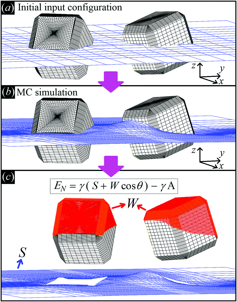 | ||
| Fig. 2 Illustrative sketch of our method. (a) A configuration Ω, i.e. the particle number, positions, and orientations (see text), and Young's contact angle θ are set as input. The blue grid shows the initial shape of the fluid–fluid interface (also defined as input), while the black grid shows the surface of the particles. (b) With our Monte Carlo approach, we compute the equilibrium shape of the fluid–fluid interface (blue grid), i.e. the solution of Young–Laplace equation with Young's Law as boundary condition. (c) From the obtained equilibrium shape of the fluid–fluid interface, we compute the total fluid–fluid surface area S (blue grid) and the particle surface area W wet by the fluid above the interface (red-colored part of the particle surface), respectively. Then, EN is obtained, see eqn (2). By repeating this procedure for different particle configurations Ω, the capillarity-induced potential EN(Ω) is obtained. Note that in this paper we show results only for cosθ = 0, so for this particular case W is not actually needed. | ||
For all the calculations shown in this work, we set cosθ = 0 in eqn (2), such that we consider the case for which the colloidal particles have equal affinity for the two fluids forming the interface, i.e. γ1 = γ2. It follows that the fluid–fluid interface at equilibrium forms an angle π/2 with the particle surfaces, that the energy EN [eqn (2)] is minimized solely by minimizing the fluid–fluid surface area S, and that the system is invariant by inverting the two fluids. Since the fluid–fluid interface is asymptotically flat and coincides with the plane z = 0 when no particle is adsorbed, it follows that either the minimum-energy solution for the particle configuration Ω and the fluid–fluid interface shape is symmetric for z → −z, or two energetically equivalent solutions, symmetric with respect to z = 0, exist.
Additional remarks
The gravitational energy of the fluid–fluid interface and the particle weight are not taken into account in the energy EN [eqn (2)], as they are negligible for the experimental systems of interest (that is, when the capillary length is much bigger than the particle size). However, we point out that gravity effects could be easily included in our numerical method. Since we use a sharp fluid–fluid interface in our model, the colloidal particle size needs to be at least a few times bigger than the diffuse interface width, typically around 1 nm.57–59 Therefore, the range of validity for the particle size in our model generally lies between an upper limit of a few μm, above which gravity may become relevant, to a lower limit of a few nm, below which the sharp approximation for the fluid–fluid interface is too inaccurate.79The line tension is also neglected, as its contribution in typical experimental systems is still unclear.60 In principle, however, also this effect could be easily included in our model, if a numerical value for the line tension is provided.
In affirming that the system reaches its minimum-energy state at equilibrium, we are assuming that pinning effects on the three-phase contact line are negligible, otherwise they would trap the system in a metastable state, preventing it from reaching the minimum of the energy. So, our predictions do not hold for experimental systems where pinning is important.61 In principle, pinning effects could be approached with our numerical method by considering solid surfaces with roughness and/or chemical heterogeneities, rather than smooth and homogeneous solid surfaces, and then studying the quasi-equilibrium dynamics of the system, but we leave this for future work.
As already mentioned, in this work we consider colloidal particles adsorbed at fluid–fluid interfaces which are flat when no particles are adsorbed. An interesting development for our numerical method is to consider fluid–fluid interfaces with a bare curvature, to verify how this affects the capillary interactions between the particles (see e.g. the experiments in ref. 27–32). We leave this application of our method for future studies.
In our model we assume that other possible interactions between the adsorbed colloidal particles (e.g. electrostatic, Casimir-like, van der Waals, etc.) are negligible when compared to capillary interactions. In Appendix B we show that this is a realistic approximation in several typical experimental systems for interparticle distances exceeding a nm or so, while at shorter distances also van der Waals forces become relevant.
In this work, we do take into account the effects of the hard-particle interactions and configurational entropy on their self-assembly, see Section III C, using approximate free-energy expressions valid for hard disks to account for packing entropy, and adding to these the capillary energy EN [eqn (2)]. We show that such entropic effects become important if the particle size is small enough. These results are summarized in the form of temperature–density phase diagrams, where different capillary-driven self-assembled phases of the adsorbed particles appear. The temperature scale is set by the dimensionless parameter Σγ/(kBT), with Σ the surface area of the particle, T the temperature and kB the Boltzmann constant. Therefore, for a given fluid–fluid surface tension γ and temperature T, these phase diagrams can be converted into a particle size-density representation. The details of these calculations will be presented in Section III C and Appendix D.
III. Results
In this section we present results for the adsorption and self-assembly of colloidal particles at a fluid–fluid interface. We consider four different shapes of the particles: sharp-edge cube, smooth-edge cube, slightly truncated-edge cube, and highly truncated-edge cube, see Fig. 1. The precise definition of the particle shapes is reported in Appendix A. In all the calculations presented here, the particle–fluid–fluid Young's contact angle is θ = π/2.First, in Section III A, we study the energy E1(Ω) [eqn (2)] of a single-adsorbed particle at the fluid–fluid interface. We show that, for all the four shapes considered, the particle induces at the equilibrium a hexapolar capillary deformation in the fluid–fluid interface height profile. Note that, as proved in ref. 53, capillarity plays a fundamental role even for the equilibrium configuration of a single-adsorbed cubic particle. This is important to point out, since a common approximation when studying the equilibrium orientation of particles at fluid–fluid interfaces is to assume an always-flat interface, i.e. to neglect capillary deformations.62–68
Then, in Section III B, we compute the energy E∞(Ω) [eqn (2)] of a periodic 2D lattice of many adsorbed particles at the fluid–fluid interface. We show that, for all the four particle shapes considered, at least three periodic arrangements of the particles exist that are energetically favorable: a hexagonal lattice, a honeycomb lattice, and a square lattice.
Finally, in Section III C, we introduce an approximated free-energy model to study the interplay between the capillary-induced potential E∞(Ω) and the entropy of the particles in these periodic lattices. As a result, we obtain a temperature–density phase diagram for each particle shape considered.
Note that some results for smooth-edge cubes were already presented in ref. 50, and are illustrated here in more detail. However, the square-lattice arrangement was not taken into account in ref. 50, while we include it in our calculations here. In addition, we present for the first time results for the other three cubic shapes (sharp-edge, slightly truncated-edge, highly truncated-edge), showing that slight variations in the particle shape affect both qualitatively and quantitatively the self-assembly of the cubes at the fluid–fluid interface.
A. Single-adsorbed particle equilibrium configuration
In Fig. 3 we show the energy E1(Ω) [eqn (2)] of a single-adsorbed particle at a fluid–fluid interface, for Young's contact angle π/2, and with, respectively: (a) a sharp-edge cubic shape, (b) a smooth-edge cubic shape, (c) a slightly truncated-edge cubic shape, and (d) a highly truncated-edge cubic shape. In the particle configuration given by Ω = (x1,y1,z1,φ1,ψ1,α1), see Fig. 1, we can neglect the energy dependence from x1, y1, and α1, because here we consider only one particle adsorbed at the fluid–fluid interface (and the interface is flat when no particle is adsorbed). Therefore, in Fig. 3 we show E1 with respect to the particle orientations φ1 and ψ1, and minimized over z1. Note that, for computing the equilibrium shape of the fluid–fluid interface to verify the dependence of E1 on z1 for each particle configuration, we keep the fluid volume constant as set by the plane z = 0. Our results show that, for any φ1 and ψ1, E1 is minimal for z1 = 0, i.e. when the particle center of mass is at the interface level, as was expected for these particle shapes and Young's contact angle π/2. | ||
| Fig. 3 Adsorption energy E1 [eqn (2)] of a single-adsorbed particle at a fluid–fluid interface, as a function of the particle orientation (φ1,ψ1) and minimized over z1, see Fig. 1, for: (a) a sharp-edge cube, (b) a smooth-edge cube, (c) a slightly truncated-edge cube, and (d) a highly truncated-edge cube (see exact definitions of these particle shapes in Appendix A). Young's contact angle is θ = π/2, and the plane z = 0 corresponds to the fluid–fluid interface when no particle is adsorbed. For any φ1 and ψ1, the obtained minimum energy value of z1 is zero. The energy E1 is plotted in units of γΣ, with Σ the particle's total surface area and γ the fluid–fluid surface tension (see text). In the insets, a 3D view of the fluid–fluid interface shape (blue grid) close to the particle (black grid) is shown for the minimum-energy configuration of the particle, as computed by our numerical method. Note that the highly truncated-edge cube (d) has two equivalent minima (i and ii) due to the particle symmetry. In the right panels we show, for the equilibrium configuration of the particles, a contour plot of the fluid–fluid interface height profile. As shown, at the equilibrium all four particle shapes are adsorbed in the 111 configuration at the interface (i.e. with one vertex pointing up) and they induce a hexapolar capillary deformation in the interface height profile. Note, however, that the magnitude of these deformations varies with respect to the particle size L. | ||
The absolute value of E1 represents the binding energy between the particle and the fluid–fluid interface, with the E1 = 0 level representing the case when the particle is not adsorbed at the interface. As shown in Fig. 3, at the particle equilibrium configuration, i.e. in the minimum of E1(φ1,ψ1), all four particle shapes have approximately the same adsorption energy E1 ≈ 0.25Σγ, with Σ the particle's total surface area and γ the fluid–fluid surface tension. Using, for example, a typical surface tension of γ = 0.01 N m−1, it follows that Σγ ≈ 350kBT for a sharp-edge cube of side L = 5 nm, and Σγ ≈ 1.5 × 10⁷kBT for a sharp-edge cube of side L = 1 μm, with T room temperature and kB the Boltzmann constant. So, the binding energy E1 is already of the order of tens-to-hundreds kBT for cubic nanoparticles, and becomes of the order of 106kBT for micrometer-sized cubes.
The equilibrium configuration at the interface of the sharp-edge cube, smooth-edge cube, and slightly truncated-edge cube is the same, and given by z1 = 0, φ1 ≈ 0.30π and ψ1 ≈ 0.25π. In analogy with ref. 50, we call this orientation of the cube the 111 configuration, as one vertex of the cube is pointing up with respect to the interface plane. The highly truncated-edge cube at the equilibrium also lies in the 111 configuration, i.e. with a vertex toward up, but slightly less tilted than the other shapes, with z1 = 0, φ1 ≈ 0.17π and ψ1 ≈ 0.25π. A second equivalent minimum appears for the highly truncated-edge cube. The two minima, however, correspond to the same equilibrium 111 configuration, within the numerical approximation used, because of the symmetry of the particle shape.
All four particle shapes induce, at their equilibrium configuration, a hexapolar capillary deformation in the fluid–fluid interface height profile, i.e. three rises and three depressions. For the sharp-edge, smooth-edge and slightly truncated-edge cubes, this hexapolar deformation is 3-fold symmetric [see the contour plots in Fig. 3(a)–(c)], like predicted for smooth-edge cubes with cosθ ≤ 0.2 in ref. 50. For the highly truncated-edge cube, the hexapolar deformation slightly loses its 3-fold symmetry, with one depression and one rise in the interface height profile slightly more spread and less intense than the remaining two rises and two depressions [see the contour plots in Fig. 3(d)]. This asymmetry, however, does not seem to have significant effects (see ESI,† Fig. S1). Anyway, the interface height profile is still symmetric for z → −z, as expected for Young's contact angle π/2. Note that the magnitude of these hexapolar deformations is different for the various particle shapes considered. The sharp-edge and smooth-edge cubes induce greater deformations, with respect to the particle size, than the truncated-edge cubes, with the highly truncated-edge cube generating significantly smaller deformations than the slightly truncated-edge cube. This influences, both qualitatively and quantitatively, the capillary interactions and self-assembly of the cubes at the fluid–fluid interface, as shown in Sections III B and C. Note that, by staying in the 111 orientation, the cubes minimize the total fluid–fluid surface area S thanks to the hexapolar capillary deformation induced in the interface. If these deformations were not taken into account, then the 111 orientation would mistakenly not result as the stable one, as proved for smooth-edge cubes in ref. 50.
B. Periodic self-assembled 2D lattices
As shown in Section III A, single-adsorbed sharp-edge, smooth-edge, slightly truncated-edge, and highly truncated-edge cubes with Young's contact angle π/2 generate a hexapolar deformation in the fluid–fluid interface height profile. Such a hexapolar deformation consists of three rises and three depressions in the interface height profile, disposed with 3-fold symmetry around the particle (with the hexapole generated by the highly truncated-edge cube slightly deviating from the exact 3-fold symmetry, see contour plots in Fig. 3). Here we study the capillary interactions between N → ∞ particles adsorbed at the fluid–fluid interface and generating such a hexapolar capillary deformation. Since our calculations suggest that, for the systems considered here, the single-particle equilibrium configuration is not affected by capillary interactions, see Appendix C, Section A, we set φi, ψi, zi for each i-th particle to the values obtained in Section III A for a single-adsorbed particle.As shown in ref. 50, if two particles generating a hexapolar deformation are at the interface, then they are attracted to each other, but only for certain relative azimuthal orientations of their hexapoles, i.e. only for certain values of α1–α2. The attractive orientations of the two hexapoles are those that allow overlap of capillary deformations with the same sign, that is overlap of rises in the height profile of the fluid–fluid interface with other rises, and overlap of depressions in the height profile of the fluid–fluid interface with other depressions. Indeed, the fluid–fluid surface area decreases by overlapping deformations of the same sign, while it increases when a rise and a depression approach each other, and, therefore, so does the energy E2 [eqn (2)]. Consequently, the two hexapole-generating particles can form two different kinds of energetically-favorable bonds: a dipole–dipole bond, when a rise-depression dipole of one hexapole overlaps with a rise-depression dipole of the other hexapole, see Fig. 4(a), and a tripole–tripole bond, when either a rise–depression–rise or a depression–rise–depression tripole of one hexapole overlaps with, respectively, a rise–depression–rise or a depression–rise–depression tripole of the other hexapole, see Fig. 4(b) and (c). Note that the tripole–tripole bonds in Fig. 4(b) and (c) are different in general. Here, however, they are energetically equivalent because Young's contact angle is π/2, and so the system is invariant by inverting the two fluids. For completeness, in the ESI† (see Fig. S1) we show, for all four particle shapes considered here, the energy E2 with respect to the particle distance for the dipole–dipole and tripole–tripole bonds, as computed through our numerical method. For example, see Fig. S1 (ESI†), at a center-of-mass distance D = 2L the pair potential per particle E2/2 − E1 is ![[scr O, script letter O]](https://www.rsc.org/images/entities/char_e52e.gif) (−0.001Σγ) for the sharp and smooth-edge cubes, and (−0.0001Σγ) for the slightly and highly truncated-edge cubes (with L the particle size, see Fig. 7, Σ the particle total surface area, and γ the fluid–fluid surface tension).
(−0.001Σγ) for the sharp and smooth-edge cubes, and (−0.0001Σγ) for the slightly and highly truncated-edge cubes (with L the particle size, see Fig. 7, Σ the particle total surface area, and γ the fluid–fluid surface tension).
 | ||
| Fig. 4 Here, we schematically represent a top view of the fluid–fluid interface with adsorbed cubic particles generating a hexapolar capillary deformation (see Fig. 3). We use red and blue spots to indicate, respectively, rises and depressions in the fluid–fluid interface height profile, while the cubic particles adsorbed in the 111 configuration, i.e. with a vertex pointing upwards, are sketched in gray (and the cube sketches refer to any of the four particle shapes considered in Fig. 3). In (a–c) we show, respectively, a dipole–dipole bond where two blue-red dipoles interact, a tripole–tripole bond where two blue-red-blue tripoles interact, and a tripole–tripole bond where two red-blue-red tripoles interact. Note that, as Young's contact angle is π/2, (b and c) are energetically equivalent. In (d and e) we sketch a honeycomb lattice where the cubes interact by the tripole–tripole bond represented in (b and c), respectively (phase h). Hence, also (d and e) are energetically equivalent. In (f) a square lattice where the cubes interact by the three bonds in (a–c) is sketched (phase s). In (g) a hexagonal lattice where the cubes interact by dipole–dipole bonds (a) is sketched (phase x). Note that, in phase h, each cube has an azimuthal orientation in the interface plane shifted by π with respect to its closest neighbors. In phase s, the azimuthal orientation of the cubes is constant along one direction of the lattice [the horizontal direction in (f)], while it is shifted by π with respect to each closest neighbor in the other direction [the vertical direction in (f)]. In phase x, all cubes have the same azimuthal orientation in the interface plane. Particle–particle distances in the lattice representations are only schematic. In the right panels of (d–g) we sketch (top) a representation of the dipole–dipole and tripole–tripole bonds formed by the cubes in the lattice, and (bottom) the lattice unit cell considered in our calculations, where the color-coding at the cell sides indicates the periodic boundary conditions we applied: sides with the same color have the same fluid–fluid interface height profile (see Appendix C, Section B, for the precise definition of the lattice unit cells). | ||
For N → ∞ the particles generate a hexapolar capillary deformation at the interface, and can self-assemble into 2D periodic lattices where dipole–dipole and tripole–tripole bonds are formed. To verify this, we calculate the (capillary) interaction energy per particle
 | (3) |
Note that the two phases h represented in Fig. 4(d) and (e) interchange for z → −z. Indeed, as Young's contact angle is π/2, either the minimum energy solution for the fluid–fluid interface shape and for the particle configuration is symmetric by inverting the two fluids, i.e. for z → −z, or, as it happens in this case, two equivalent solutions, being one equal to the other for z → −z, exist. As they are equivalent, in our calculations we consider only one of the two possible h phases. One could wonder whether the honeycomb lattice of phase h is actually just an incomplete hexagonal lattice of phase x. This is not the case, since in phase x the particle are dipole–dipole interacting, while in phase h they are tripole–tripole interacting. In addition, an energy barrier exists for the particles in phase h that frustrates the adsorption of more hexapole-generating particles in the holes of the honeycomb lattice, and also that prevents the tripole–tripole bonds to become dipole–dipole bonds. This is shown in detail in Appendix C, Section C.
In Fig. 5 we show, for the various particle shapes and phases h, s, x, the plot of ηẼ∞(η), that is the interaction energy per particle [see eqn (3)] multiplied by the normalized particle density η, where η = 1 for the close-packed phase x. Here ηẼ∞(η) is plotted in units of γ/δx, with δx the particle density of the close-packed phase x (see Table 2) and γ the fluid–fluid surface tension. As shown, ηẼ∞(η) decreases by increasing the particle density η, for each phase considered, proving that it is energetically favorable for the particles to self-assemble into the phases h, s and x. Although qualitatively similar, the interaction strength Ẽ∞ of the various lattice phases is quantitatively quite different for the four particle shapes considered, with a difference of an order of magnitude going from the sharp-edge cube to the highly truncated-edge cube (see also the ESI,† Fig. S2, where we show the same results of Fig. 5, but plotting Ẽ∞, instead of ηẼ∞, in units of Σγ, i.e. the same energy units used in Fig. 3). These quantitative differences have important consequences for the self-assembly of the particles at the interface, as we will show in Section III C. Since ηẼ∞(η) is an energy per unit area plotted with respect to the particle density, we can use the common tangent construction69 to individuate where phase coexistence occurs, obtaining, from the results of Fig. 5, that the close-packed phase x (i.e. at η = 1) coexists with an empty phase (i.e. η = 0), for any density η of particles at the fluid–fluid interface. So, one could conclude that, in equilibrium, the particles at the fluid–fluid interface self-assemble into the close-packed phase x, while the close-packed phases h and s are only metastable states. However, as pointed out in ref. 50, this reasoning on the basis of solely the capillary energy Ẽ∞(η) is only correct if the entropy of the particles can be ignored, which is only the case in the low-temperature or large-particle regime, i.e. if γΣ/(kBT) is sufficiently large. In Section III C, we will add the contribution of the particle entropy to the (capillary) interaction energy Ẽ∞(η), showing that any of the three phases h, s and x can be the equilibrium phase, either alone on the whole fluid–fluid interface or phase-coexisting with the others, by tuning the dimensionless parameter γΣ/(kBT) and the particle density.
 | ||
| Fig. 5 (Capillary) Interaction energy per particle Ẽ∞ [eqn (3)] with respect to the particle density η (which is normalized such that η = 1 for the close-packed phase x), as computed through our numerical method for 2D periodic lattices of particles adsorbed at a fluid–fluid interface, with each particle generating a hexapolar deformation (see Fig. 3). Green refers to a honeycomb lattice [phase h, see Fig. 4(d) and (e)], blue to a square lattice [phase s, see Fig. 4(f)], and pink to a hexagonal lattice [phase x, see Fig. 4(g)]. The particle shape is (a) a sharp-edge cube, (b) a smooth-edge cube, (c) a slightly truncated-edge cube, and (d) a highly-truncated edge cube (see exact definitions of these particle shapes in Appendix A). In the graphs, the squares are the results from our numerical simulations, obtained for various particle densities, i.e. using different sizes of the lattice unit cell. The full lines represent a fit of our numerical data, for the phases h, s, x, of the form Aα·(η)Bα, where Aα and Bα are the fit parameters, with α = h, s, x, respectively, and their obtained values are reported in Appendix C, Table 3. The vertical dotted lines indicate the close-packed density for the honeycomb lattice (phase h, in green), for the square lattice (phase s, in blue), and for the hexagonal lattice (phase x, in pink). In these graphs Ẽ∞ is multiplied by the particle density η and plotted in units of γ/δx, with δx the particle density of the close-packed phase x (see Table 2) and γ the fluid–fluid surface tension. From the common tangent construction,69 see black dotted line, it follows that at equilibrium the close-packed phase x coexists with an empty phase (i.e. a phase with η = 0), for any density η of particles at the fluid–fluid interface. In the ESI,† Fig. S2, the same results are shown, but plotting Ẽ∞, instead of ηẼ∞, in units of Σγ, i.e. the same energy units used in Fig. 3. Contour plots of the fluid–fluid interface height profile, for the various lattices and particle shapes, are shown in Appendix C for different unit cell sizes (see Fig. 10). | ||
C. Temperature–density phase diagrams
As shown in Section III B, particles adsorbed at a fluid–fluid interface generate a hexapolar capillary deformation and can self-assemble into various 2D periodic lattices: a honeycomb lattice [phase h, see Fig. 4(d) and (e)], a square lattice [phase s, see Fig. 4(f)], and a hexagonal lattice [phase x, see Fig. 4(g)]. On the basis of solely the (capillary) interaction energy per particle Ẽ∞ [eqn (3)] of these lattices, one would conclude that at equilibrium the particles at the interface self-assemble into the close-packed phase x (in coexistence with an empty phase, see Fig. 5). However, this is correct only when the particle entropy, due to the configurational entropy and hard-particle interactions, is negligible. Here we introduce an approximated model to estimate the interplay between capillary interactions and particle entropy.For each phase of the adsorbed particles at the fluid–fluid interface, we write the total (free) energy F as
| F(N,A,T) = EN(N,A) + FS(N,A,T), | (4) |
We consider the free energy density
 | (5) |
 | (6) |
To estimate the FS(η,T)/(Aγ) term in eqn (6) for the four particle phases f, h, s, and x, we use analytical and numerical results from the literature for 2D systems of hard disks. If we were considering a pure hard-body fluid, treating our adsorbed particles as hard disks would be, of course, a rough approximation, since the shape of the hard bodies is a key parameter. Here, however, we are considering the interplay between capillary and entropic contributions, instead of a system with only hard interactions. So, using well-known equations for hard-disk systems to estimate FS(η,T) should be a fair approximation here. Only if entropy dominates over capillarity, i.e. Σγ ≪ kBT, this argument is not valid anymore. However, we are not interested in this regime, since the adsorption energy of a particle at the interface is E1 ≈ −0.25Σγ for all the particle shapes (see Fig. 3), that is the particles are not stable anymore at the interface already for Σγ ≲ 10kBT. In addition, to improve our model, we add to FS(η,T) a correction term −NkBTlnZor to include the rotational entropy, since in the crystal phases the particles have a fixed azimuthal orientation in the interface plane, while hard disks can freely rotate. The orientational partition function Zor is calculated assuming that the particle azimuthal orientations are constrained by a rotational spring potential, and the spring constant, due to capillary interactions, is calculated using our numerical method. The explicit expressions of FS(η,T) used for the various particle phases, and related calculations, are reported in Appendix D.
From the plots of the free-energy density f(η,T) [eqn (6)] of the particle phases f, h, s, and x, with respect to η, and at different values of Σγ/(kBT), we calculate where phase coexistence occurs by using common tangent constructions (see Appendix D for details). The obtained results are summed up in the temperature–density phase diagrams in Fig. 6 for (a) sharp-edge cubes, (b) smooth-edge cubes, (c) slightly truncated-edge cubes, and (d) highly truncated-edge cubes. In this temperature–density representation, the tie lines that connect the coexisting phases are horizontal. We observe a stable fluid phase depicted in light blue at low densities and a stable honeycomb, square and hexagonal phase depicted green, dark blue and pink, respectively, at sufficiently high densities. The two-phase regions are shown in gray. Firstly, note that in the low temperature or big particle regime, that is Σγ/(kBT) → ∞, i.e. when the particle entropy is negligible, we find that a close-packed phase x coexists with an almost-empty phase f, in agreement with the results of Fig. 5 where particle entropy was not included. Then, by increasing Σγ/(kBT), that is by increasing the effects of particle entropy, we find that also the lattice phases h and s can be equilibrium phases of the particles at the interface, either as a single phase in a tiny (almost singular) density regime, or coexisting with other phases in a large density regime. The most interesting result revealed by these phase diagrams is that the Σγ/(kBT) regime in which the honeycomb phase h and the square phase s can form drastically varies by changing the particle shape. For example, for smooth-edge and sharp-edge cubes, the interval where the honeycomb phase h occurs is around Σγ/(kBT) ≈ 300–400, while for slightly and highly truncated-edge cubes this interval is, respectively, around Σγ/(kBT) ≈ 800–2000 and Σγ/(kBT) ≈ 1000–3000. This means, for example, that at a fixed temperature and fluid–fluid surface tension, bigger particles are necessary to form the honeycomb phase h if using truncated-edge cubes rather than smooth-edge or sharp-edge cubes. For instance, setting T to room temperature and the fluid–fluid surface tension to the typical value γ = 0.01 N m−1, it follows that sharp-edge and smooth-edge cubes can self-assemble into a honeycomb lattice only for L ≈ 4–5 nm, while slightly and highly truncated-edge cubes can form a honeycomb lattice only for L ≈ 8–12 nm and L ≈ 10–16 nm, respectively. Note that these experimental parameters match very well with the experiments in ref. 47–49, where 5-to-10 nm sized nanocrystals of cubic shape are observed to form square, hexagonal, and honeycomb lattices at the fluid–fluid interface. The main reason for the different Σγ/(kBT) regime in which the phases h and s occur for the different particle shapes, is in the different intensity of the hexapolar capillary deformations, with respect to the particle size, generated by the different particles (see Fig. 3). Another important factor for determining the equilibrium phase of the various particle shapes is the contact distance of the particles in the lattices, that is the close-packed density for each phase. More details on this are reported in Appendix D. Another important result that emerges from Fig. 6 is that for sharp-edge cubes the square lattice phase s is never thermodynamically stable, and only the phases h and x are possible at equilibrium. The main reason for this seems to lie in the contact distance for the tripole–tripole bonds between the cubes, which is much larger than for the other shapes, although other parameters play a role as well in this (see more details in Appendix D). Note, however, that the hard-disk approximation used to estimate the entropic part of the free energy F(N,A,T) [eqn (4)] is worse for the sharp-edge cubes than for the other shapes. Using a better approximation could induce slight variations in the phase diagram of the sharp-edge cubes, at least for high T. Plots of the free-energy density f [eqn (6)], with respect to the particle density η and for some values of Σγ/(kBT), are reported for the particle phases f, h, s, and x in the ESI,† see Fig. S3–S6, where the common tangents we calculated are also shown.
 | ||
| Fig. 6 Temperature–density phase diagram for adsorbed (a) sharp-edge cubes, (b) smooth-edge cubes, (c) slightly truncated-edge cubes, and (d) highly-truncated edge cubes at a fluid–fluid interface. The left vertical axis is γΣ/(kBT), with γ the fluid–fluid surface tension, Σ the total surface area of a particle, kB the Boltzmann constant, and T the temperature (note that the low temperature or big particle limit is in the verse toward down of the vertical axis). The right vertical axis represents the corresponding value of the particle size L (see exact definition in Appendix A) at room temperature and using a typical surface tension γ = 0.01 N m−1. The horizontal axis is the particle density η, normalized such that η = 1 for the close-packed x-phase. The colored areas indicate where a pure phase exists on the whole fluid–fluid interface: light-blue for phase f (disordered phase), green for phase h (honeycomb lattice), blue for phase s (square lattice), and pink for phase x (hexagonal lattice). The gray areas indicate where coexistence between two phases occurs, and the red symbols mark the triple points where three phases coexist. The Young contact angle considered here is π/2, so the cubes are always adsorbed at the interface in the 111 configuration (i.e. with a vertex toward up, see Section III A). | ||
IV. Conclusion
In this paper we have studied the capillary interactions and self-assembly of cubic particles adsorbed at a flat fluid–fluid interface. The capillary deformations and interactions of the particles at the interface are computed using a recently introduced Monte Carlo method53 (see results in Sections III A and B), first for a single-adsorbed particle and then for a periodic array. Then, the self-assembly at the interface is predicted using an approximated free-energy model where capillarity is coupled with the particle configurational entropy and the hard-particle interactions (see Section III C). As a result, see Fig. 6, we obtained temperature–density phase diagrams where different 2D lattice phases (honeycomb, square, hexagonal) appear as thermodynamically stable for different regimes of particle density, size, and temperature.In particular, we have investigated the effects of slightly tuning the cubic shape, considering sharp-edge cubes, smooth-edge cubes, slightly truncated-edge cubes, and highly truncated-edge cubes. We have shown that such slight variations of the particle shape significantly affect, both qualitatively and quantitatively, the self-assembly of the cubes at the fluid–fluid interface. These results extend previously presented calculations50 where only smooth-edge cubes were considered, and the capillary-induced square lattice phase was not taken into account. This work is a step forward into fully understanding the experiments in ref. 47–49, where hexagonal, honeycomb and square lattices of adsorbed nanocubes are actually observed. Interestingly, in these works capillarity is not taken into account to justify the observed structures, rather ligand adsorption and van der Waals forces between specific facets of the nanocubes are suggested. Our work strongly suggests, instead, that capillarity is the leading force responsible for the observed structures, although we cannot exclude that other forces may play a role as well at short (almost-contact) particle–particle distances. In fact, our phase diagram even features a well-defined parameter range in which the honeycomb lattice is to be expected, and this region is consistent with the experiments in ref. 47–49. It is important to point out that in this work we considered only the case of Young's contact angle θ = π/2, that is when the particles adsorbed at the interface have the same affinity with the two fluids. In ref. 50 it is predicted that, for cosθ ≥ 0.3, a single-adsorbed cube at the equilibrium lies in the flat orientation at the interface – the same orientation observed in ref. 47–49 for the nanocubes forming a square lattice – without generating significant capillary deformations. However, ref. 50 also shows that, for a single-adsorbed cube, a metastable vertex-up configuration inducing a hexapolar capillary deformation exists for cosθ ≥ 0.3. Therefore, if cosθ ≥ 0.3, self-assembly into honeycomb, hexagonal and square lattice phases could still be energetically favorable for many adsorbed nanocubes, possibly in coexistence with phases where the nanocubes lie flat at the fluid–fluid interface. We leave the case θ ≠ π/2 and the verification of this hypothesis to future work, possibly including also the case of different Young's contact angles associated to different facets of the cubes.
Finally, it is interesting to point out that also in other experiments70 hexagonal lattices of 10-to-15 nm side cubes have been observed at a fluid–fluid interface, with the cubes oriented in the 111 configuration (i.e. vertex toward up) at the interface. Although these experiments are complicated by the presence of nanocubes also in the bulk of one of the fluids (while in our model the particles are only at the fluid–fluid interface), the observed structures at the fluid–fluid interface are in complete agreement with our predictions based on capillary interactions.
Conflicts of interest
There are no conflicts to declare.Appendix A: particle shapes
Here we report the exact definition of the particle shapes considered in this paper. The sharp-edge cube, see Fig. 7(a), is, simply, a standard cube with side L. The smooth-edge cube, see Fig. 7(b), is defined by the super-quadratic parametric equation | (7) |
 | (8) |
 | (9) |
| (tL/2,−tL/2,L/2); (−tL/2,tL/2,L/2); |
| (−tL/2,−tL/2,L/2); (tL/2,tL/2,L/2); |
| (L/2,tL/2,tL/2); (L/2,−tL/2,tL/2); |
| (tL/2,−tL/2,−L/2); (−L/2,tL/2,tL/2); |
| (−L/2,−tL/2,tL/2); (−tL/2,−L/2,tL/2); |
| (tL/2,L/2,tL/2); (tL/2,−L/2,tL/2); |
| (−tL/2,L/2,tL/2); (L/2,tL/2,−tL/2); |
| (L/2,−tL/2,−tL/2); (−tL/2,L/2,−tL/2); |
| (−L/2,tL/2,−tL/2); (tL/2,L/2,−tL/2); |
| (tL/2,−L/2,−tL/2); (−tL/2,−L/2,−tL/2); |
| (−L/2,−tL/2,−tL/2); (tL/2,tL/2,−L/2); |
| (−tL/2,tL/2,−L/2); (−tL/2,−tL/2,−L/2). | (10) |
 | ||
| Fig. 7 3D view of the particle surface (black grid) for the four particle shapes considered in this work: (a) a sharp-edge cube, (b) a smooth-edge cube, (c) a slightly truncated-edge cube, and (d) a highly truncated-edge cube. See exact definition of these surfaces in the text. | ||
| Particle shape | Σ/L2 |
|---|---|
| Sharp-edge cube | 6.00 |
| Smooth-edge cube | 5.65 |
| Slightly truncated-edge cube | 5.06 |
| Highly truncated-edge cube | 4.05 |
Appendix B: Casimir-like and van der Waals interactions
To verify the accuracy of our model for the desired system, it is important to establish whether other possible particle–particle interactions are important compared to capillary interactions. In this Appendix we address this point for van der Waals interactions and Casimir like forces.About van der Waals interactions, we show here that, for typical experimental parameters, they are relevant only in the limit of very small particles and very small (almost contact) particle–particle distances. In Fig. 8 we show the van der Waals potential ΦvdW between two spheres of diameter σ ≡ 2R, with respect to the particle center-of-mass distance D ≡ d + σ, calculated with a Hamaker–de Boer approach71 as
 | (11) |
438kBT for σ = 100 nm and Σγ ≈ 764kBT for σ = 10 nm. Compared with the capillary interactions per particle in Fig. 5 (see also Fig. S1 and S2, in the ESI,† where the energy is expressed in units of Σγ), van der Waals interactions are completely negligible for spheres with σ ≈ 100 nm, while they may become relevant for spheres with σ ≈ 10 nm, i.e. with a size comparable to the nanocubes in ref. 47–49. Note, however, that the range of the capillary interactions goes far beyond the range of the van der Waals forces (compare Fig. 5 and 8). So, for such experiments, capillarity seems to be the leading driving force for the long-range order of the observed structures, while van der Waals forces could become relevant for (almost) touching particles.
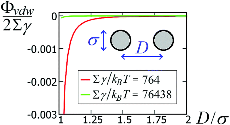 | ||
| Fig. 8 van der Waals interaction potential ΦvdW between two spheres of diameter σ as a function of the center-of-mass distance D [see eqn (11)], for a system with Hamaker constant A = 0.15 eV, in units of Σγ, with γ = 0.01 N m−1 and Σ = πσ2 the sphere surface area. | ||
Other particle–particle interactions that are not included in our calculations, but could arise for adsorbed particles at fluid–fluid interfaces, are Casimir-like forces.73–75 These interactions are due to the thermal fluctuations (capillary waves) experienced by the fluid–fluid interface equilibrium profile. We show here that these forces are indeed negligible compared to the capillary interactions induced by the hexapolar deformations in the systems considered in this work. Following ref. 76, we can express the fluctuation-induced potential between two spheres adsorbed at a fluid–fluid interface as
 | (12) |
 | (13) |
Appendix C: additional information on the 2D periodic lattices of the particle phases h, s, x
A. On the single-particle equilibrium configuration
Here we verify whether the particle equilibrium configuration computed in Section III A for a single-adsorbed particle changes or not when the particle experiences capillary interactions with other particles. We consider, see Fig. 9, two almost-touching tripole–tripole interacting particles, and we set the particle configuration zi, ψi, φi, with i = 1, 2 (see Fig. 1), to the equilibrium values found in Section III A for a single-adsorbed particle. Then, in Fig. 9 we report how E2 [eqn (2)] behaves by varying, respectively, z1, ψ1, and φ1. As shown in the plots, the minimum energy value of each of these parameters coincides with the value found in Section III A for a single-adsorbed particle. Hence, these results indicate that capillary interactions do not affect significantly the equilibrium configuration of the particles, at least for the systems considered here, where Young's contact angle is π/2. Therefore, in the lattice phases h, s and x defined in Section III B we can assume that zi, ψi, φi for each i particle are the same as computed for a single-adsorbed particle in Section III A. In Fig. 9 we considered only smooth-edge cubes and highly truncated-edge cubes, since the same results reasonably apply for the remaining two particle shapes. These results give also an idea of the strength of the capillary forces keeping the particles in their equilibrium configuration. Note that, in the numerical calculations for the equilibrium shape of the fluid–fluid interface considered here, the fluid volume was set constant (and given by the fluid–fluid interface when coinciding with the plane z = 0), since the single-particle equilibrium configuration was in principle unknown, and so we needed to study the energy dependence from the particle center of mass height at the interface. | ||
Fig. 9 Energy E2 [eqn (3)] for two tripole–tripole interacting particles, with respect to the configuration of a single particle, in units of Σγ (with Σ the total surface area of a particle and γ the fluid–fluid surface tension). We consider (a) two smooth-edge cubes with configuration z1 = z2 = 0, ψ1 = ψ2 = π/4, φ1 = φ2 = 0.3π, α1 = 0, α2 = π and (b) two highly truncated-edge cubes with configuration z1 = z2 = 0, ψ1 = ψ2 = π/4, φ1 = φ2 = 0.17π, α1 = 0, α2 = π (see Fig. 1). The center-of-mass distance  between the two particles is in (a) D = 1.6L and in (b) D = 1.35L, so in both cases D only slightly exceeds the contact distance. Young's contact angle is π/2. We plot E2, as computed by our numerical method, obtained by varying, respectively, z1, ψ1, and φ1. As shown, the equilibrium values for z1, ψ1, and φ1 are the same found for a single-adsorbed particle in Section III A, even if here there are two interacting particles. In (c and d) we show a contour plot of the interface height profile when z1, ψ1, and φ1 are at the equilibrium for the two tripole–tripole interacting particles considered in (a) and (b), respectively. The plane z = 0 corresponds to the fluid–fluid interface when no particle is adsorbed. between the two particles is in (a) D = 1.6L and in (b) D = 1.35L, so in both cases D only slightly exceeds the contact distance. Young's contact angle is π/2. We plot E2, as computed by our numerical method, obtained by varying, respectively, z1, ψ1, and φ1. As shown, the equilibrium values for z1, ψ1, and φ1 are the same found for a single-adsorbed particle in Section III A, even if here there are two interacting particles. In (c and d) we show a contour plot of the interface height profile when z1, ψ1, and φ1 are at the equilibrium for the two tripole–tripole interacting particles considered in (a) and (b), respectively. The plane z = 0 corresponds to the fluid–fluid interface when no particle is adsorbed. | ||
B. On the definition of the lattice unit cells
We define here the lattice unit cell and the particle configuration Ω (see Section II) for the particle phases h, s, and x defined in Section III B.For phase h, the unit cell [see sketch in Fig. 4(d) and (e)] is a rectangle with vertexes of Cartesian coordinates 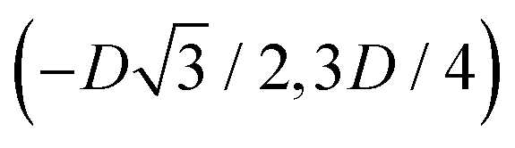 ,
,  ,
,  , and
, and  , in the z = 0 plane. Periodic boundary conditions are applied to the cell sides: the half-side from
  to (0,−3D/4) has the same fluid–fluid interface height profile of the half-side from (0,3D/4) to
  , the half-side from (0,−3D/4) to
 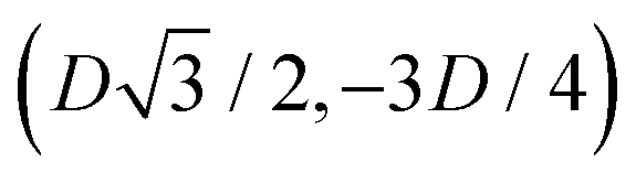 has the same fluid–fluid interface height profile of the half-side from
  to (0,3D/4), and the two remaining opposite sides of the cell have the same fluid–fluid interface height profile. In the cell there are N = 2 particles with configuration (xi,yi,αi), for i = 1, 2, given by
  and
and  , where the sign choice determines whether we are considering the phase h in Fig. 4(d) or the energetically equivalent phase h in Fig. 4(e).
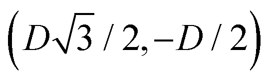
For phase s, the unit cell [see sketch in Fig. 4(f)] is a rectangle with vertexes of Cartesian coordinates (−Dd/2,−Dt), (Dd/2,−Dt), (Dd/2,Dt), and (−Dd/2,Dt) in the z = 0 plane. Periodic boundary conditions are applied to the cell sides: opposite sides of the square cell have the same fluid–fluid interface height profile. In the cell there are N = 2 particles with configuration (xi,yi,αi), for i = 1, 2, given by (0,−Dt/2,0) and (0,Dt/2,π).
For phase x, the unit cell [see sketch in Fig. 4(g)] is a hexagon in the z = 0 plane with vertexes of Cartesian coordinate (0,−D), (0,D),  ,
,  ,
,  , and
, and  . Periodic boundary conditions are applied to the cell sides: opposite sides of the hexagonal cell have the same fluid–fluid interface height profile. In the cell there is N = 1 particle with position and orientation (x1,x2,α1) given by (0,0,0).
The remaining degrees of freedom for the particle configuration in each lattice unit cell (i.e. φi, ψi, zi, with i = 1, 2 for phases h and s, and i = 1 for phase x) are fixed by the values found in Section III A for a single-adsorbed particle. Note that, for each i-th particle in the lattice phases, its αi = 0 orientation is when the line corresponding to the particle vertical axis, see Fig. 1, is parallel to the x = 0 plane and with non-negative derivative in y.
In the lattice unit cell of the phases h and x, the parameter D is the center-of-mass distance between two closest-neighbor particles of the lattice. In the lattice unit cell of the phase s, the parameters Dd and Dt are the center-of-mass distances between two closest neighbor particles in the dipole–dipole bond direction of the lattice and in the tripole–tripole bond direction of the lattice, respectively (see Fig. 4). By tuning D for the phases h and x, and Dd, Dt for the phase s, we regulate the lattice spacing, and therefore the particle density in the lattice. The normalized particle density η is given by 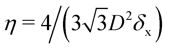 for the phase h, η = 1/(DdDtδx) for the phase s, and
 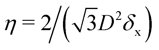 for the phase x, where δx is the density N/A (with N number of particles and A area) of the phase x lattice unit cell when the particles are at their contact distance, see Table 2. The values we estimated for the particle contact distances in the phases h, s, and x are reported in Table 2, for the various particle shapes. Note that, for the square lattice (phase s), the contact distance value for Dd, i.e. Ddc, is smaller than the contact distance value for Dt, i.e. Dtc, for any particle shape (see Table 2). Therefore, we use a square lattice unit cell, i.e. Dd = Dt, when Dt ≥ Dtc. Instead, for higher particle densities, we use a rectangular cell with Dt = Dtc and Ddc < Dd < Dtc. We verified that using a rectangular unit cell, rather than square, also for lower particle densities does not affect our results, see ESI,† Fig. S7.
 , δs = 1/(DdcDtc), and
 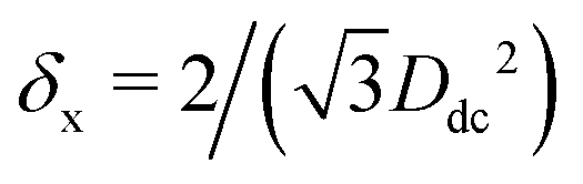 , respectively, and is reported here in units of Σ−1, with Σ the particle total surface area. The particle shape is (a) a sharp-edge cube, (b) a smooth-edge cube, (c) a slightly truncated-edge cube, and (d) a highly-truncated edge cube
| D tc/L | D dc/L | δ h Σ | δ s Σ | δ x Σ | |
|---|---|---|---|---|---|
| (a) | 1.63 | 1.42 | 1.724 | 2.580 | 3.431 |
| (b) | 1.55 | 1.40 | 1.810 | 2.604 | 3.329 |
| (c) | 1.43 | 1.24 | 1.918 | 2.864 | 3.800 |
| (d) | 1.17 | 1.15 | 2.276 | 3.008 | 3.534 |
C. On the capillary interaction energy
For the various particle phases and shapes, in Fig. 5 we showed ηẼ∞(η), where Ẽ∞ is the (capillary) interaction energy [eqn (3)] and η the normalized particle density (such that η = 1 for the close-packed phase x). The numerical data we obtained for ηẼ∞(η), for the phases h, s, x, were fitted with Aα·(η)Bα, where Aα and Bα are the fit parameters (with α = h, s, x, respectively for each phase). The values we obtained are reported in Table 3. In Fig. 10 we show the contour plot of the interface height profile, as obtained from our numerical method, in the unit cell of the phases h, s, and x, for different sizes of the cell and for the various particle shapes.| δ x A h/γ | B h | δ x A s/γ | B s | δ x A x/γ | B x | |
|---|---|---|---|---|---|---|
| (a) | −0.4052 | 4.1171 | −0.1592 | 3.8466 | −0.1141 | 3.6701 |
| (b) | −0.2062 | 3.6879 | −0.1213 | 3.6709 | −0.0773 | 2.9911 |
| (c) | −0.1151 | 3.9437 | −0.0477 | 3.8577 | −0.0275 | 3.2012 |
| (d) | −0.0350 | 3.9222 | −0.0206 | 4.3770 | −0.0150 | 4.1576 |
 | ||
| Fig. 10 Contour plot of the fluid–fluid interface height profile, as obtained by our numerical method, in a unit cell of the particle lattice phase h, s, and x (from left to right, respectively). The particle shape used is (a) a sharp-edge cube, (b) a smooth-edge cube, (c) a slightly truncated-edge cube, and (d) a highly-truncated edge cube. Note that periodic boundary conditions are applied to the lattice unit cells, as described in the text (see also sketches in Fig. 4). Each lattice unit cell is shown for a given particle density η, where η = 1 corresponds to the close-packed phase x. The plane z = 0 corresponds to the fluid–fluid interface when no particle is adsorbed. The particle size L is defined in Appendix A. | ||
Concerning the numerical calculations for the equilibrium shape of the fluid–fluid interface in the results of Fig. 5, the initial volume of the fluids was set by the interface level when coinciding with the plane z = 0. Then, during the Monte Carlo simulations to find the interface equilibrium shape, the volume was not constrained to be constant (so it was free to evolve to its minimum energy value). However, since the center of mass height zi for each i particle was set to its minimum energy value zi = 0 (as proved for a single-adsorbed particle in Section III A and for interacting particles in Section A of this Appendix), the initial fluid volume we set is also the minimum-energy volume, so constraining the volume to remain constant in our simulations would have made no difference for the computed interface equilibrium shape. The same argument applies for the calculations in the next section and in Fig. 12 of Appendix D.
D. On the (meta)stability of the honeycomb lattice
While the square lattice (phase s) is clearly different from the hexagonal and honeycomb lattices (phases x and h), one could wonder whether the honeycomb lattice of the phase h is just an incomplete hexagonal lattice of the phase x, i.e. whether the capillary energy per particle of the honeycomb lattice can be lowered just by adding another particle in each honeycomb “hole”. Here we show that this is not the case and the honeycomb lattice of the phase h is (at least locally) stable from evolving into an hexagonal lattice, even in the limit of negligible particle entropy. For these calculations, we consider only smooth-edge cubes, since the same results reasonably apply, at least qualitatively, for the other cubic particle shapes.In Fig. 11(a) we consider a unit cell of the honeycomb lattice of the phase h (see definition in Section B of this Appendix), where the equilibrium azimuthal orientations α1 and α2 of the two particles are shifted by +ω and −ω, respectively. In the plot, we show the interaction energy per particle Ẽ∞ [eqn (3)] with respect to ω. As indicated by the colored arrows and the sketches in Fig. 11(b), by increasing ω, i.e. by rotating the particle azimuthal orientations in opposite directions (clockwise for one particle, and counterclockwise for the other), we shift from a honeycomb lattice with depression–rise–depression tripole–tripole interactions, to a honeycomb lattice with dipole–dipole interactions, then to a honeycomb lattice with rise–depression–rise tripole–tripole interactions, then again to a honeycomb lattice with dipole–dipole interactions, and so on. The honeycomb lattice with dipole–dipole interactions is actually the hexagonal lattice of phase x, but with half of the particles removed to form a honeycomb. So, it can further reduce its energy per particle by filling the holes in the lattice with particles. Instead, the honeycomb lattice with tripole–tripole interactions is the actual phase h. As shown, the energy Ẽ∞ reaches a minimum when the particles are in the phase h configuration, while is maximum when they are in the incomplete phase x configuration, therefore (locally) preventing the phase h to evolve in a configuration that is unstable toward evolving into the phase x. Since in these calculations only capillarity is taken into account, and particle entropy is not included, this holds in the low temperature or big particle regime. If particle entropy is important, then as shown in Section III C the honeycomb lattice of phase h can become not only locally but also globally stable. Finally, in Fig. 11(c) we show that for a honeycomb lattice of the phase h, i.e. with tripole–tripole interacting cubes, it is energetically unfavorable to adsorb additional cubes in the honeycomb holes. Here we show the interaction energy per particle Ẽ6 and Ẽ7, with respect to the particle distance, for, respectively, six particles with configuration (xi,yi,αi), for i = 1,…6, given by  ,
,  , (D,0,π),
  ,
,  , (−D,0,0), and seven particles with configuration (xi,yi,αi), for i = 1,…6, given as before and for i = 7 given by (0,0,π). For each particle i, the values of zi, ψi, φi are the same as found in Section III A for a single-adsorbed particle. In both cases, the six external particles [see Fig. 11(c)] interact with one another by tripole–tripole interactions, i.e. as in the phase h. As shown, at least for small particle distances, Ẽ6 is lower than Ẽ7, proving that for the phase h it is energetically unfavorable to adsorb additional cubes in the honeycomb holes. The reason is that the tripole–tripole interacting cubes of phase h generate a multi-particle interaction of capillary deformations with the same sign in the honeycomb holes, frustrating the addition of another hexapole-generating cube.
 | ||
| Fig. 11 (a) Interaction energy Ẽ∞ [eqn (3)] for the honeycomb lattice of phase h (see definition in Section B of this Appendix), where the equilibrium azimuthal orientations α1 and α2 of the two particles are shifted by +ω and −ω, respectively. The energy is plotted in units of Σγ, with Σ the total surface area of one particle and γ the fluid–fluid surface tension. The particle density in the lattice is η = 0.38. The different colored arrows, corresponding to different ω, indicate the different phases in which the lattice evolves by tuning ω. Starting from a honeycomb lattice with depression–rise–depression tripole–tripole interactions at ω = 0 (green arrow), we obtain a honeycomb lattice with dipole–dipole interactions at ω = π/6 (light-blue arrow), then a honeycomb lattice with rise–depression–rise tripole–tripole interactions at ω = 2π/6 (orange arrow), then again to a honeycomb lattice with dipole–dipole interactions at ω = 3π/6 (light-blue arrow), and so on. A contour plot of the fluid–fluid interface height profile in the lattice cell for ω = 0 (i) and ω = π/6 (ii) is shown in the insets. (b) Graphical representations of the various phases in which the honeycomb lattice evolves, where the red/blue spots indicate rises/depressions in the fluid–fluid interface height profile, and the cubes are sketched in gray. (c) Interaction energy per particle ẼN [eqn (3)] with respect to the center of mass particle distance D for, respectively, six and seven particles with configuration as described in the text. In the insets we show, for both cases, a contour plot of the fluid–fluid interface height profile for D = 1.65L. | ||
Appendix D: free-energy calculations for the phase diagrams
Here, we report the explicit expressions used to estimate the term FS(η,T)/(Aγ) in the free energy density f(η,T) [see eqn (6)] defined in Section III C, for all the particle phases f, h, s, and x. The particle density η is normalized such that η = 1 for the close-packed phase x, A is the fluid–fluid interface total area when no particle is adsorbed, γ is the fluid–fluid surface tension, and T is the temperature.For the four particle phases, respectively f, h, s, and x, we assume
| F(f)S(N,A,T) ≈ Ffhd(N,A,T), | (14) |
F(h)S(N,A,T) ≈ Ffhd(N,A,T) − NkBT![[thin space (1/6-em)]](https://www.rsc.org/images/entities/i_char_2009.gif) lnZ(h)or, lnZ(h)or, | (15) |
| F(s)S(N,A,T)≈ Ffhd(N,A,T) − NkBTlnZ(s)or, | (16) |
| F(x)S(N,A,T) ≈ Fxhd(N,A,T) − NkBTlnZ(x)or. | (17) |
From scaled-particle theory77 we have
 | (18) |
| Particle shape | Ω/Σ | τ 2/Σ | Ω/τ2 |
|---|---|---|---|
| Sharp-edge cube | 0.296 | 4.101 | 0.072 |
| Smooth-edge cube | 0.276 | 3.834 | 0.072 |
| Slightly truncated-edge cube | 0.265 | 3.667 | 0.072 |
| Highly truncated-edge cube | 0.243 | 3.365 | 0.072 |
From the numerical results in ref. 78 we obtain
 | (19) |
In the three lattice phases h, s, and x, each particle i has a fixed azimuthal orientation αi in the interface plane, while, instead, hard disks can freely rotate. To take this into account in FS(η,T)/(Aγ), we add the (free) energy −NkBTlnZor due to the azimuthal orientation of the particles. The one-particle orientational partition function Zor is defined assuming that the energy cost for a particle to rotate by ω from its equilibrium azimuthal orientation αi is
 | (20) |
 | (21) |
 | ||
Fig. 12 Rotational spring constant C for the particle phase h (green), s (blue) and x (pink), and for (a) a sharp-edge cube, (b) a smooth-edge cube, (c) a slightly truncated-edge cube, and (d) a highly-truncated edge cube. For the phase h, we consider a lattice unit cell (see Appendix C) where the azimuthal orientation α1 of the first particle is shifted by ω from its equilibrium value, while the second particle orientation is kept at its equilibrium value α2, and we use our numerical method to compute EN [eqn (2)] with respect to ω, for various η. For the phases x and s we proceed analogously, but considering, respectively, seven particles with configuration (xi,yi,αi), for i = 1,…7, given by  , ,  , (D,0,0), , (D,0,0),  , ,  , (−D,0,0), (0,0,ω), and nine particles with configuration (xi,yi,αi), for i = 1,…9, given by (−D,−D,0), (−D,0,π), (−D,D,0), (0,−D,0), (0,D,0), (D,−D,0), (D,0,π), (D,D,0), (0,0,π + ω). The corresponding particle density η(D) for these particle configurations is the same reported in Appendix C for the lattice unite cells of phase x and s, respectively. The αi = 0 orientation of each i-th particle is defined as in Appendix C for the lattice phases. The remaining degrees of freedom of the particle configuration (i.e. φi, ψi, zi, for i = 1,…7 and i = 1,…9, respectively) are fixed by the values found in Section III A for a single-adsorbed particle. In the graphs shown here, the squares are the values of C, for the various particle phases, obtained by fitting EN(ω) − EN(ω = 0) with U(ω) [eqn (20)], see Fig. S9–S12 of the ESI.† The full lines represent a fit of our numerical data with A·e−B/η, where A and B are the fit parameters (and their values, obtained from the fit, are reported in Table 5). The vertical dotted lines indicate the close-packed density, i.e. when the particles are at their contact distance, for the honeycomb lattice (phase h, in green), for the square lattice (phase s, in blue), and for the hexagonal lattice (phase x, in pink). Here, C is plotted in units of Σγ, with Σ the total surface area of one particle and γ the fluid–fluid surface tension. , (−D,0,0), (0,0,ω), and nine particles with configuration (xi,yi,αi), for i = 1,…9, given by (−D,−D,0), (−D,0,π), (−D,D,0), (0,−D,0), (0,D,0), (D,−D,0), (D,0,π), (D,D,0), (0,0,π + ω). The corresponding particle density η(D) for these particle configurations is the same reported in Appendix C for the lattice unite cells of phase x and s, respectively. The αi = 0 orientation of each i-th particle is defined as in Appendix C for the lattice phases. The remaining degrees of freedom of the particle configuration (i.e. φi, ψi, zi, for i = 1,…7 and i = 1,…9, respectively) are fixed by the values found in Section III A for a single-adsorbed particle. In the graphs shown here, the squares are the values of C, for the various particle phases, obtained by fitting EN(ω) − EN(ω = 0) with U(ω) [eqn (20)], see Fig. S9–S12 of the ESI.† The full lines represent a fit of our numerical data with A·e−B/η, where A and B are the fit parameters (and their values, obtained from the fit, are reported in Table 5). The vertical dotted lines indicate the close-packed density, i.e. when the particles are at their contact distance, for the honeycomb lattice (phase h, in green), for the square lattice (phase s, in blue), and for the hexagonal lattice (phase x, in pink). Here, C is plotted in units of Σγ, with Σ the total surface area of one particle and γ the fluid–fluid surface tension. | ||
| A h/(Σγ) | B h | A s/(Σγ) | B s | A x/(Σγ) | B x | |
|---|---|---|---|---|---|---|
| (a) | 9.874 | 1.000 | 20.121 | 1.455 | 63.782 | 2.141 |
| (b) | 17.308 | 1.372 | 39.269 | 2.095 | 32.567 | 2.345 |
| (c) | 4.062 | 1.160 | 2.238 | 1.152 | 2.640 | 1.181 |
| (d) | 2.244 | 1.313 | 1.299 | 1.286 | 2.748 | 1.598 |
We rewrite the expressions for FS(η,T)/(Aγ) for the various particle phases [eqn (14)–(17)] with respect to the dimensionless parameter Σγ/(kBT), using kBTN/(Aγ) = δxΣηkBT/(Σγ), where Σ is the particle total surface area, and δx is the particle density of the close-packed phase x and is reported in units of Σ−1 in Table 2 for the various particle shapes. Then, we plot for each phase the free energy density f(η,T) [eqn (6)] with respect to the particle density η and for different values of Σγ/(kBT). Using common tangent constructions69 between the free energy density plots of the different particle phases, we find the particle density values where phase coexistence occurs, for each value of Σγ/(kBT) considered. The results for each particle shape are shown in the temperature–density phase diagrams in Section III C. In the ESI,† see Fig. S3–S6, we show, for all the particle shapes, the plots of f(η,T) for the various particle phases and for some values of Σγ/(kBT), highlighting the common tangents we calculated.
To further illustrate that the approximations used to estimate the particle entropy in our model do not significantly affect the results, in the ESI† we show, see Fig. S8 (ESI†), the temperature–density phase diagram, for the smooth-edge cubes, as obtained using the crystal hard disk free energy Fxhd [eqn (19)] instead of the fluid hard disk free energy Ffhd [eqn (18)] in the entropic free energies F(h)S [eqn (15)] and F(s)S [eqn (16)] of the particle phases h and s. The result is almost identical to the phase diagram shown in Fig. 6(b).
Acknowledgements
The authors acknowledge financial support by the “Nederlandse Organisatie voor Wetenschappelijk Onderzoek” (NWO) Vici Grant and by the Marie Curie Initial Training Network “Soft Matter at Aqueous Interfaces” (SOMATAI). This work is part of the D-ITP consortium, a program of the NWO that is funded by the Dutch Ministry of Education, Culture and Science (OCW).References
- F. Bresme and M. Oettel, J. Phys.: Condens. Matter, 2007, 19, 413101 CrossRef CAS PubMed.
- S. Coertjens, R. De Dier, P. Moldenaers, L. Isa and J. Vermant, Langmuir, 2017, 33, 2689 CrossRef CAS PubMed , PMID: 28241120.
- P. Pieranski, Phys. Rev. Lett., 1980, 45, 569 CrossRef CAS.
- B. Park et al. , Particle-Stabilized Emulsions and Colloids: Formation and Applications, Soft Matter Series, Royal Society of Chemistry, 2014 Search PubMed.
- B. P. Binks, Langmuir, 2017, 33, 6947–6963 CrossRef CAS PubMed.
- S. Dasgupta, T. Auth and G. Gompper, J. Phys.: Condens. Matter, 2017, 29, 373003 CrossRef CAS PubMed.
- J. Vermant, Nature, 2011, 476, 286 CrossRef CAS PubMed.
- P. J. Yunker, T. Still, M. A. Lohr and A. G. Yodh, Nature, 2011, 476, 308 CrossRef CAS PubMed.
- S. Jiang, et al. , Chem. Soc. Rev., 2017, 46, 3792 RSC.
- S. Sacanna, W. K. Kegel and A. P. Philipse, Phys. Rev. Lett., 2007, 98, 158301 CrossRef CAS PubMed.
- M. G. Basavaraj, S. Vandebril, J. Fransaer and J. Vermant, Soft Matter, 2009, 5, 1717 RSC.
- E. Dickinson, Trends Food Sci. Technol., 2012, 24, 4 CrossRef CAS.
- R. Aveyard, Soft Matter, 2012, 8, 5233 RSC.
- F. Günther, S. Frijters and J. Harting, Soft Matter, 2014, 10, 4977 RSC.
- M. Vis, et al. , ACS Macro Lett., 2015, 4, 965 CrossRef CAS.
- M. Zanini, et al. , Nat. Commun., 2017, 8, 15701 CrossRef CAS PubMed.
- M. A. Fernandez-Rodriguez, B. P. Binks, M. A. Rodriguez-Valverde, M. A. Cabrerizo-Vilchez and R. Hidalgo-Alvarez, Adv. Colloid Interface Sci., 2017, 247, 208–222 CrossRef CAS PubMed.
- H. Katepalli, V. T. John, A. Tripathi and A. Bose, J. Colloid Interface Sci., 2017, 485, 11 CrossRef CAS PubMed.
- J. C. Loudet and B. Pouligny, Eur. Phys. J. E: Soft Matter Biol. Phys., 2011, 34, 76 CrossRef CAS PubMed.
- A. Kumar, B. J. Park, F. Tu and D. Lee, Soft Matter, 2013, 9, 6604 RSC.
- S. Coertjens, P. Moldenaers, J. Vermant and L. Isa, Langmuir, 2014, 30, 4289 CrossRef CAS PubMed.
- G. Morris, K. Hadler and J. Cilliers, Curr. Opin. Colloid Interface Sci., 2015, 20, 98 CrossRef CAS.
- A. Kozina, S. Ramos, P. Díaz-Leyva and R. Castillo, J. Phys. Chem. C, 2016, 120, 16879 CAS.
- M. Zanini and L. Isa, J. Phys.: Condens. Matter, 2016, 28, 313002 CrossRef PubMed.
- L. C. Bradley, W.-H. Chen, K. J. Stebe and D. Lee, Curr. Opin. Colloid Interface Sci., 2017, 30, 25 CrossRef CAS.
- T. G. Anjali and M. G. Basavaraj, Langmuir, 2017, 33, 791 CrossRef CAS PubMed.
- W. T. M. Irvine, V. Vitelli and P. M. Chaikin, Nature, 2010, 468, 947 CrossRef CAS PubMed.
- M. Cavallaro, L. Botto, E. P. Lewandowski, M. Wang and K. J. Stebe, PNAS, 2011, 108, 20923 CrossRef CAS PubMed.
- W. T. M. Irvine and V. Vitelli, Soft Matter, 2012, 8, 10123 RSC.
- C. Blanc, et al. , Phys. Rev. Lett., 2013, 111, 058302 CrossRef PubMed.
- D. Ershov, J. Sprakel, J. Appel, M. A. Cohen Stuart and J. van der Gucht, PNAS, 2013, 110, 9220 CrossRef CAS PubMed.
- I. B. Liu, N. Sharifi-Mood and K. J. Stebe, 2017, arXiv:1710.05258v1 [cond-mat.soft].
- N. Senbil and A. D. Dinsmore, Soft Matter, 2017 10.1039/C7SM01548H.
- R. Di Leonardo, F. Saglimbeni and G. Ruocco, Phys. Rev. Lett., 2008, 100, 106103 CrossRef CAS PubMed.
- L. Yao, et al. , Soft Matter, 2013, 9, 779 RSC.
- R. McGorty, J. Fung, D. Kaz and V. N. Manoharan, Mater. Today, 2010, 13, 34 CrossRef CAS.
- E. M. Furst, PNAS, 2011, 108, 20853 CrossRef CAS PubMed.
- A. D. Law, M. Auriol, D. Smith, T. S. Horozov and D. M. A. Buzza, Phys. Rev. Lett., 2013, 110, 138301 CrossRef PubMed.
- M. Lee, M. Xia and B. J. Park, Materials, 2016, 9, 138 CrossRef PubMed.
- Q. Xie, G. B. Davies and J. Harting, Soft Matter, 2016, 12, 6566 RSC.
- S.-M. Kang, et al. , Soft Matter, 2016, 12, 5847 RSC.
- D.-G. Lee, P. Cicuta and D. Vella, Soft Matter, 2017, 13, 212 RSC.
- I. B. Liu, N. Sharifi-Mood and K. J. Stebe, 2017, arXiv:1710.05258.
- D. Vanmaekelbergh, Nano Today, 2011, 6, 419 CrossRef CAS.
- W. Beugeling, et al. , Nat. Commun., 2015, 6, 1 Search PubMed.
- W. H. Evers, et al. , Nat. Commun., 2015, 6, 8195 CrossRef CAS PubMed.
- H. Evers, et al. , Nano Lett., 2013, 13, 2317 CrossRef PubMed.
- M. P. Boneschanscher, et al. , Science, 2014, 344, 1377 CrossRef CAS PubMed.
- J. J. Geuchies, et al. , Nat. Mater., 2016, 15, 1248 CrossRef CAS PubMed.
- G. Soligno, M. Dijkstra and R. van Roij, Phys. Rev. Lett., 2016, 116, 258001 CrossRef PubMed.
- J. L. Peters, et al. , Chem. Mater., 2017, 29, 4122 CrossRef CAS PubMed.
- L. D. Landau and E. M. Lifshitz, Statistical Physics – Part I, Pergamon Press, 3rd revised and enlarged edition, 1980, p. 531 Search PubMed.
- G. Soligno, M. Dijkstra and R. van Roij, J. Chem. Phys., 2014, 141, 244702 CrossRef PubMed.
- G. Soligno, Droplets, capillary interactions, and self-assembly from the equilibrium shape of fluid–fluid interfaces, PhD thesis, Utrecht University, 2017, ch. 4, ISBN: 978-94-6332-124-2 Search PubMed.
- I. Dević, et al. , Langmuir, 2017, 33, 2744 CrossRef PubMed.
- M. Kamp, et al. , J. Phys. Chem. C, 2017, 121, 19989 CAS.
- J. Gao and W. L. Jorgensen, J. Phys. Chem., 1988, 92, 5813 CrossRef CAS.
- I. L. Carpenter and W. J. Hehre, J. Phys. Chem., 1990, 94, 531 CrossRef CAS.
- D. S. Walker and G. L. Richmond, J. Am. Chem. Soc., 2007, 129, 9446 CrossRef CAS PubMed.
- A. Amirfazli and A. Neumann, Adv. Colloid Interface Sci., 2004, 110, 121 CrossRef CAS PubMed.
- A. Wang, R. McGorty, D. M. Kaz and V. N. Manoharan, Soft Matter, 2016, 12, 8958 RSC.
- J. de Graaf, M. Dijkstra and R. van Roij, J. Chem. Phys., 2010, 132, 164902 CrossRef PubMed.
- B. J. Park and D. Lee, Soft Matter, 2012, 8, 7690 RSC.
- B. J. Park and D. Lee, ACS Nano, 2012, 6, 782 CrossRef CAS PubMed.
- A. R. Morgan, et al. , Soft Matter, 2013, 9, 487 RSC.
- W. van der Stam, et al. , Nano Lett., 2014, 14, 1032 CrossRef CAS PubMed.
- B. Peng, et al. , Soft Matter, 2014, 10, 9644 RSC.
- N. Ballard and S. A. F. Bon, J. Colloid Interface Sci., 2015, 448, 533 CrossRef CAS PubMed.
- G. Soligno, Droplets, capillary interactions, and self-assembly from the equilibrium shape of fluid–fluid interfaces, PhD thesis, Utrecht University, 2017, Sec. 5.6.5, ISBN: 978-94-6332-124-2.
- J. J. Choi, K. Bian, W. J. Baumgardner, D.-M. Smilgies and T. Hanrath, Nano Lett., 2012, 12, 4791 CrossRef CAS PubMed.
- P. C. Hiemenz and R. Rajagopalan, Principles of Colloid and Surface Chemistry, Marcel Dekker, Inc., 3rd edn, 1997 Search PubMed.
- D. V. Talapin and E. V. Shevchenko, Nano Lett., 2007, 7, 1213 CrossRef CAS PubMed.
- D. Bonn, et al. , Phys. Rev. Lett., 2009, 103, 156101 CrossRef PubMed.
- A. Gambassi and S. Dietrich, Phys. Rev. Lett., 2010, 105, 059601 CrossRef PubMed.
- D. Bonn, G. Wegdam and P. Schall, Phys. Rev. Lett., 2010, 105, 059602 CrossRef.
- M. Oettel, A. Domnguez and S. Dietrich, Phys. Rev. E: Stat., Nonlinear, Soft Matter Phys., 2005, 71, 051401 CrossRef CAS PubMed.
- Y. Rosenfeld, Phys. Rev. A: At., Mol., Opt. Phys., 1990, 42, 5978 CrossRef CAS.
- D. A. Young and B. J. Alder, J. Chem. Phys., 1979, 70, 473 CrossRef CAS.
- U. Gupta, T. Hanrath and F. A. Escobedo, Phys. Rev. Materials, 2017, 1, 055602 CrossRef.
Footnote |
| † Electronic supplementary information (ESI) available. See DOI: 10.1039/c7sm01946g |
| This journal is © The Royal Society of Chemistry 2018 |