 Open Access Article
Creative Commons Attribution 3.0 Unported Licence
Adaptive free energy sampling in multidimensional collective variable space using boxed molecular dynamics
Mike
O'Connor
ab,
Emanuele
Paci
c,
Simon
McIntosh-Smith
b and
David R.
Glowacki
*ab
aSchool of Chemistry, University of Bristol, Bristol BS8 1TS, UK. E-mail: drglowacki@gmail.com
bDepartment of Computer Science, University of Bristol, Bristol BS8 1UB, UK
cAstbury Centre for Structural Molecular Biology, University of Leeds, Leeds, UK
First published on 28th June 2016
Abstract
The past decade has seen the development of a new class of rare event methods in which molecular configuration space is divided into a set of boundaries/interfaces, and then short trajectories are run between boundaries. For all these methods, an important concern is how to generate boundaries. In this paper, we outline an algorithm for adaptively generating boundaries along a free energy surface in multi-dimensional collective variable (CV) space, building on the boxed molecular dynamics (BXD) rare event algorithm. BXD is a simple technique for accelerating the simulation of rare events and free energy sampling which has proven useful for calculating kinetics and free energy profiles in reactive and non-reactive molecular dynamics (MD) simulations across a range of systems, in both NVT and NVE ensembles. Two key developments outlined in this paper make it possible to automate BXD, and to adaptively map free energy and kinetics in complex systems. First, we have generalized BXD to multidimensional CV space. Using strategies from rigid-body dynamics, we have derived a simple and general velocity-reflection procedure that conserves energy for arbitrary collective variable definitions in multiple dimensions, and show that it is straightforward to apply BXD to sampling in multidimensional CV space so long as the Cartesian gradients ∇CV are available. Second, we have modified BXD to undertake on-the-fly statistical analysis during a trajectory, harnessing the information content latent in the dynamics to automatically determine boundary locations. Such automation not only makes BXD considerably easier to use; it also guarantees optimal boundaries, speeding up convergence. We have tested the multidimensional adaptive BXD procedure by calculating the potential of mean force for a chemical reaction recently investigated using both experimental and computational approaches – i.e., F + CD3CN → DF + D2CN in both the gas phase and a strongly coupled explicit CD3CN solvent. The results obtained using multidimensional adaptive BXD agree well with previously published experimental and computational results, providing good evidence for its reliability.
1 Introduction
The solution to a wide range of problems that can be addressed with molecular simulation consists fundamentally of determining rate coefficients. For example, biochemical systems rely on a delicate balance of rate coefficients within larger coupled kinetic networks.1 Similarly, bulk oxidation timescales in atmospheric chemistry2 and combustion3 (required to predict pollutant lifetimes, or to optimize an engine) are linked to detailed kinetic networks comprised of a wide range of elementary kinetic steps.4 With developments in both statistical mechanics and electronic structure theory, it is now possible to identify the important stationary points on a molecular potential energy surface (PES),5 and carry out accurate calculations of the energy and partition function at each point. This enables extremely accurate calculations of the rates at which small molecules undergo structural changes, in either canonical or microcanonical ensembles.6 However, calculating accurate rate coefficients for larger molecules (e.g., enzymes, long-chain hydrocarbon fuels, unsaturated volatile organic pollutants, etc.) remains an outstanding challenge for a number of reasons: (1) it remains difficult to calculate an accurate PES along a given path, (2) there is a combinatorial explosion in the number of paths with increasing system dimensionality, and (3) the conformational flexibility inherent in larger molecular systems makes it very difficult to calculate accurate partition functions. Particularly as a result of the latter two challenges, the calculation of rate coefficients in complex systems tends to not to focus on stationary points, but rather on free energy surfaces along a particular path between states, typically defined in terms of a small set of collective variables (CVs). In cases where it is a good assumption that the full system dynamics along a particular path is mostly associated with changes in a small set of CVs, then the maximum on the free energy surface may be utilized to calculate rate coefficients in the Eyring equation.7 In cases where this is not a good assumption, an additional correction in the form of the so-called ‘recrossing coefficient’ is typically applied.8,9In this paper, we present a relatively simple adaptive algorithm for discovering minimum free energy pathways between states in a multidimensional space of CVs, which can then be used to calculate rate coefficients in complex systems. There is strong evidence within computational complexity theory that problems of this sort are NP-complete10–12 – i.e., it is possible to verify (within polynomial time) whether any proposed solution is indeed a solution, but there is no known polynomial time algorithm to find a solution in the first place. This has rather profound consequences for how we think about free energy path sampling in complex molecular systems: the emphasis is less on finding an algorithm which is well-suited to every type of rare event problem, but rather on having access to a flexible range of methods which can be practically used to tackle different conformational search problems.
‘Boxed Molecular Dynamics’ (BXD),13–16 a method we have been actively involved in developing over the last few years, allows one to obtain both thermodynamic and kinetic information from the same run, producing data that produces a Markov master equation.1,4,14,17 BXD can be formulated so as to conserve energy, accelerating NVE simulations as well as NVT simulations. As a result of these features, BXD has been successfully utilized to provide microscopic insight into a range of problems within condensed phase chemistry.15,16,18–30 The fact that BXD preserves the dynamics (unlike umbrella sampling, where dynamics is lost) has been experimentally confirmed for a growing set of systems.18,20–22,24 The fundamental idea in BXD is to accelerate dynamics simulations by introducing a set of hard boundaries within the hyper-dimensional configuration space of the system being simulated. When a trajectory passes a boundary, those components of the velocity vector that take the trajectory across the boundary are reflected. The statistics of reflections at the boundary of the box are subsequently used to renormalize the results. Within BXD, ‘boxes’ refer to the configuration space domain between a particular set of boundaries. In principle, it is possible to implement boundaries which depend on the 6n dimensional phase space of Cartesian coordinates and momenta (where n is the number of atoms); however, in practice the original implementations of BXD utilized one-dimensional CVs in configuration space.
BXD falls within a class of sampling methods in which molecular configuration space is divided into a set of boundaries (also called interfaces or hypersurfaces), and short trajectories are run between boundaries. These methods (e.g., milestoning,31,32 forward flux sampling,33,34 transition interface sampling,35 nonequilibrium umbrella sampling,36 and others37–39) have yet to displace umbrella sampling40 as the most widely used method to determine free energies (or potentials of mean force), but in fact they have a number of features which we believe make them more attractive than umbrella sampling: (1) because they do not require modification of the potential energy function, they perturb the dynamics far less than umbrella sampling; (2) they allow for exact renormalization of the results in each box (unlike the iterative numerical WHAM scheme typically utilized to renormalize umbrella sampling results); (3) they require specification of fewer parameters than umbrella sampling (i.e., BXD only requires specifying a boundary location; umbrella sampling requires specifying the umbrella position and force constant); (4) they can provide both thermodynamic (free energy) and kinetic (rate) data simultaneously; (5) unlike umbrella sampling, they provide results which are in fact dynamically meaningful; and (6) it is possible to rigorously define the regimes in which the accelerated dynamics they provide map onto the results that would have been obtained using standard unbiased simulations with standard initial conditions sampling strategies.
An important concern with these methods is how to generate boundaries (analogous to the umbrella sampling issue of how best to choose ‘umbrella’ potentials). In a broad range of molecular simulation studies, boundaries (or umbrella potentials) are located along a particular set of CVs which align with the intuition of the investigator (i.e., “user”). For example, in enzyme catalysis, it is usually possible to highlight a few key bonds as being particularly important; similarly in a drug binding study, it is often possible to identify a few key motions as particularly important to binding. Such user intuition is not a panacea: it may in fact fail to identify important CVs, and there are potential pitfalls41 owing to the fact that it is often extremely difficult to find good CVs.42 Nevertheless, for understanding dynamics in hyperdimensional systems, user ‘intuition’ as to the important CVs usually constitutes an important guess as to where to initiate sampling and make practical progress in a simulation study.
With BXD's implementation in the CHARMM molecular simulation package,43 it has found application to a range of chemical systems. These applications have highlighted two important issues: (1) the BXD velocity reflection procedure must be generalized to deal with a wider range of CVs than the relatively small subset with which it is currently compatible; (2) with the implementation of a wider range of CVs, BXD must be formulated in a way that can automatically identify optimal boundaries in multi-dimensional collective variable space. The reason for the latter point is that BXD in multi-dimensional CV space requires specifying a large number of parameters. The number of parameters required scales as NCV × NB, where NCV is the number of collective variables, and NB is the number of boundaries (NB is typically between 10 and 100 in systems studied so far). For relatively small systems where NCV = 1 and which require no more than ∼10 boundaries, a user can typically keep track of the number of parameters requiring specification; however, for larger systems where NCV > 1, the number of parameters which requires specification rapidly expands beyond what even an expert can keep track of, becoming extremely tedious (if not altogether impossible). By automating the boundary selection scheme outlined in this paper using an adaptive algorithm, we avoid these problems entirely, and we also guarantee the specification of optimal boundaries. Adaptive sampling strategies have been previously explored in the context of umbrella sampling,44,45 force biasing,46 weighted ensemble sampling,39 transition interface sampling,47 accelerated molecular dynamics,48 metadynamics49,50 and steered MD.51
BXD's robustness arises in part from the fact that it generates free energy profiles which are largely insensitive to the location of boundaries, so long as the typical transit time from one boundary of the box to the other is larger than the system's characteristic decorrelation timescale.13,14 This is in fact the only ‘hard-and-fast’ rule which must be satisfied in order for BXD to yield physically meaningful results: the average time between boundary reflections in any given box must be larger than the system's characteristic dynamical decorrelation timescale in that region of the free energy surface.14 This rule places a lower limit on the allowed distance between any box's boundaries; otherwise, ballistic reflection between box boundaries will occur, and the results are meaningless. So long as the boundaries are far enough apart to avoid problems related to dynamical decorrelation, then the choice of box boundaries is flexible, and the BXD results do not depend on boundary location.
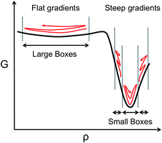
However, the computational efficiency of BXD (i.e., the speed at which it converges a free energy or a rate calculation) does depend on the boundary placement. For maximum efficiency, the boundaries should be placed close enough together so that a typical trajectory will visit the boundaries of any given box in a reasonable amount of time. Optimally placed boundaries will result in faster convergence. This is an issue that has become particularly apparent as we have attempted to use BXD to accelerate dynamics obtained from on-the-fly electronic structure theory, and also in condensed phase reactions, where force evaluations are very expensive. Our experience to date has shown that ‘user-selected’ box boundaries are often far from ideal, and can result in wasted clock cycles, a point which is easily understood from Scheme 1. In regions with a large gradient, boxes should be smaller, given that an unbiased trajectory free to sample the box is more likely to get trapped downhill rather than travel uphill, while in flatter regions that have a small gradient, the boxes can be larger, given that an unbiased trajectory will more readily sample wide regions of the configuration space. Scheme 1 therefore allows us to understand how clock cycles are wasted as a result of two common boundary-selection pitfalls: (1) large boxes in a region of the free energy surface with steep gradients, or (2) small boxes in a relatively flat region of the free energy surface. In the former case, the trajectory will rarely visit high free energy configurations within the box, and convergence will be slow. In the latter case, clock cycles are wasted on constraining sampling in flat regions of the free energy surface that the trajectory would have naturally visited anyway – i.e., the boundaries actually slow down an intrinsic sampling rate which was already satisfactory. Scheme 1 highlights a final important point – i.e., sampling on any given free energy path often requires boxes of varying sizes, with the size of the box inversely related to the gradient of the free energy surface along a particular coordinate, which is generally unknown in advance. Box boundary placement is also sensitive to the local friction regime in which the dynamical process of interest takes place (a point discussed in further detail below). In general, efficient sampling in high friction environments (e.g., a chemical reaction occurring in a solvent) requires closely spaced boundaries, while boundaries in low friction environments (e.g., a chemical reaction in the gas phase) are farther apart.
In this paper, we outline an extension of BXD to multidimensional CV space, and an automated procedure that adaptively generates optimal BXD hypersurfaces to sample dynamical pathways within a user-specified multidimensional CV space. The underlying idea guiding this approach is simple, and exploits one of the key advantages of BXD compared to a method like umbrella sampling: because the underlying dynamics are in fact meaningful, ‘on-the-fly’ analysis of their information content is in fact the most reliable guide to boundary placement. This philosophy allows us to use BXD for generating optimal boundaries in multidimensional applications, which may be subsequently used to accelerate rare events or carry out free energy sampling. We also report on results using this multi-dimensional adaptive BXD scheme to accelerate free energy sampling along the F + CD3CN → DF + CD2CN reactive pathway, in both CD3CN solvent and in the gas phase. This system constitutes a stringent test of the methodology, owing to the extreme asymmetry of the PES either side of the transition state (TS) – e.g., similar to that shown in Scheme 1. The results are in good agreement with previous experimental and modelling studies, providing good evidence for the reliability of our extended BXD algorithm. We believe that the adaptive scheme described in this article may be useful to other methods that rely on sampling between configuration space interfaces.
2 Theoretical framework
2.1 BXD along a single collective variable
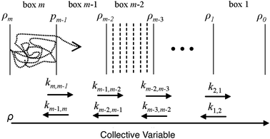
BXD is an exact extension of transition state theory,13,14 with origins in Intramolecular Dynamics Diffusion Theory (IDDT),52–56 which describes the motion of a trajectory along a reaction coordinate in terms of a diffusional equation or equivalent Langevin equation. BXD was initially formulated in order to accelerate dynamics by introducing a series of constraints along a one-dimensional collective variable, which provide a series of ‘boxes’ within which to lock the trajectory, as illustrated in Fig. 1. The region defined by the collective variable ρ is split into m boxes by the introduction of m + 1 user defined constraints. The trajectory is constrained within each box, which allows one to sample regions that would otherwise be visited only rarely.The trajectory constraint procedure involves an elastic collision procedure applied at the boundaries, which works as follows: whenever the next time step in the dynamics would result in the trajectory crossing the boundary, the trajectory is reset to the previous step, and a velocity inversion (i.e., reflection) procedure is applied to those atoms that contribute to the definition of the collective variable. For a given box i bounded by ρi and ρi−1, the rate coefficient for transfer from box i to i − 1 is determined by the inverse of the mean first passage time (MFPT) 〈τ〉. The simplest way to compute this is to keep track of the number of times the trajectory has undergone velocity transformation at each boundary, hi,i−1, along with the total amount of time, ti, that the trajectory spends within box i. This gives the rate coefficient for transfer from box i to box i − 1 as follows:
 | (1) |
The equilibrium constant between box i and box i − 1 may then be obtained from equilibrium statistical mechanics as
 | (2) |
 | (3) |
Having determined the probability of residing in any specific box according to (3), it is then possible to determine p(ρ) to arbitrary resolution by renormalizing the statistics within each box using histogram binning. Letting pi(ρ) be the probability of a particular value of ρ observed in box i, estimated by histogram binning from a sample within the box, then the probability of residing anywhere along the reaction coordinate defined by the boxes is given by
| p(ρ) = pi(ρ) × pi. | (4) |
Since only the box-to-box rate coefficients need to be computed, the length of time the trajectory needs to spend in each box is only determined by how long it takes for these rate coefficients to converge. The BXD method of partitioning the configuration space allows regions that are poorly sampled in standard MD trajectories to be isolated within a box and sampled independently, which lends itself well to parallelisation on modern cluster architectures. Alternatively, it is easy to formulate the BXD algorithm so that a given trajectory – after a specified number of reflection events at a particular boundary – is allowed to proceed to the next box, as illustrated in Fig. 1. Such a ‘box-to-box’ strategy allows trajectories to scan over adjacent boxes until convergence is achieved.
2.2 Extending BXD to multidimensional collective variable space
In this section, we present a generalisation of BXD to multidimensional collective variables. For a system of N atoms, we define![[r with combining right harpoon above (vector)]](https://www.rsc.org/images/entities/i_char_0072_20d1.gif) (t) ∈
(t) ∈ ![[Doublestruck R]](https://www.rsc.org/images/entities/char_e175.gif) 3N to be the vector of Cartesian coordinates of atoms in the system, and
3N to be the vector of Cartesian coordinates of atoms in the system, and ![[v with combining right harpoon above (vector)]](https://www.rsc.org/images/entities/i_char_0076_20d1.gif) (t) ∈
(t) ∈ ![[Doublestruck R]](https://www.rsc.org/images/entities/char_e175.gif) 3N to be the vector of corresponding velocities. A collective variable at some time t is a function s(t) of
3N to be the vector of corresponding velocities. A collective variable at some time t is a function s(t) of ![[r with combining right harpoon above (vector)]](https://www.rsc.org/images/entities/i_char_0072_20d1.gif) (t) and
(t) and ![[v with combining right harpoon above (vector)]](https://www.rsc.org/images/entities/i_char_0076_20d1.gif) (t). In cases where one wants to characterize the dynamics of a molecular system at some time t using M collective variables, then the CV space may be represented as an M-dimensional vector
(t). In cases where one wants to characterize the dynamics of a molecular system at some time t using M collective variables, then the CV space may be represented as an M-dimensional vector ![[s with combining right harpoon above (vector)]](https://www.rsc.org/images/entities/i_char_0073_20d1.gif) (t) = [s1(t), s2(t), …, sM(t)], where M is generally much less than N. In the simplest case, where M = 1,
(t) = [s1(t), s2(t), …, sM(t)], where M is generally much less than N. In the simplest case, where M = 1, ![[s with combining right harpoon above (vector)]](https://www.rsc.org/images/entities/i_char_0073_20d1.gif) (t) is often referred to as a reaction coordinate. In its original implementation, BXD partitioned a one-dimensional collective variable space into an ordered set of zero-dimensional points along the reaction coordinate. An intuitive route to generalising BXD is thus to partition the M-dimensional CV space into a series of (M − 1) dimensional boundaries, which is a strategy that follows naturally from BXD's origins in transition state theory.54,57 For example, a two-dimensional CV space may be partitioned by an ordered set of lines, a three-dimensional CV space by an ordered set of planes, and so on – to the general case of hyperplanes. Within an M-dimensional collective variable space
(t) is often referred to as a reaction coordinate. In its original implementation, BXD partitioned a one-dimensional collective variable space into an ordered set of zero-dimensional points along the reaction coordinate. An intuitive route to generalising BXD is thus to partition the M-dimensional CV space into a series of (M − 1) dimensional boundaries, which is a strategy that follows naturally from BXD's origins in transition state theory.54,57 For example, a two-dimensional CV space may be partitioned by an ordered set of lines, a three-dimensional CV space by an ordered set of planes, and so on – to the general case of hyperplanes. Within an M-dimensional collective variable space ![[s with combining right harpoon above (vector)]](https://www.rsc.org/images/entities/i_char_0073_20d1.gif) (t) = [s1(t), s2(t), …, sM(t)], any given BXD boundary Bj may be defined as a plane in Hessian normal form – i.e., in terms of a unit norm
(t) = [s1(t), s2(t), …, sM(t)], any given BXD boundary Bj may be defined as a plane in Hessian normal form – i.e., in terms of a unit norm ![[n with combining right harpoon above (vector)]](https://www.rsc.org/images/entities/i_char_006e_20d1.gif) = [n1, n2, …, nM] and a constant Dj:
= [n1, n2, …, nM] and a constant Dj: | (5) |
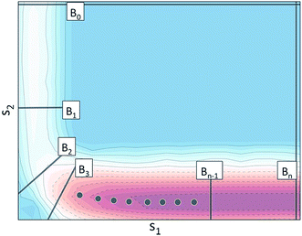
Using the notation outlined above, Fig. 2 schematically illustrates a set of BXD boundaries that one might choose in order to partition a system defined in terms of two collective variables.
2.3 General velocity reflection procedure in multidimensional collective variable space
Having specified a set of boundaries which partition the space of collective variables into smaller regions, a standard MD trajectory is performed within boundaries Bj and Bj−1 at every step, the collective variable vector![[s with combining right harpoon above (vector)]](https://www.rsc.org/images/entities/i_char_0073_20d1.gif) (t) is computed, and the velocities and positions of the previous time step are stored. For times t where the trajectory crosses either boundary Bj or Bj−1, a velocity reflection procedure is applied to constrain the trajectory so that it does not cross the boundary. In what follows, we focus on the velocity reflection procedure to be used for reflecting off multi-dimensional boundaries of the sort defined in eqn (5), generalizing the one-dimensional velocity reflection procedure outlined in our previous BXD papers to multidimensional collective variable space.
(t) is computed, and the velocities and positions of the previous time step are stored. For times t where the trajectory crosses either boundary Bj or Bj−1, a velocity reflection procedure is applied to constrain the trajectory so that it does not cross the boundary. In what follows, we focus on the velocity reflection procedure to be used for reflecting off multi-dimensional boundaries of the sort defined in eqn (5), generalizing the one-dimensional velocity reflection procedure outlined in our previous BXD papers to multidimensional collective variable space.
Within the space of collective variables, eqn (5) specifies that a BXD boundary Bj is defined in terms of a unit norm ![[n with combining right harpoon above (vector)]](https://www.rsc.org/images/entities/i_char_006e_20d1.gif) j ∈
j ∈ ![[Doublestruck R]](https://www.rsc.org/images/entities/char_e175.gif) M, which lies a distance Dj from the origin. The function ϕ(
M, which lies a distance Dj from the origin. The function ϕ(![[r with combining right harpoon above (vector)]](https://www.rsc.org/images/entities/i_char_0072_20d1.gif) (t)) =
(t)) = ![[s with combining right harpoon above (vector)]](https://www.rsc.org/images/entities/i_char_0073_20d1.gif) (t)·
(t)·![[n with combining right harpoon above (vector)]](https://www.rsc.org/images/entities/i_char_006e_20d1.gif) j + Dj provides a measure of how far the system is from a particular boundary at time t, with changes in the sign of ϕ(
j + Dj provides a measure of how far the system is from a particular boundary at time t, with changes in the sign of ϕ(![[r with combining right harpoon above (vector)]](https://www.rsc.org/images/entities/i_char_0072_20d1.gif) (t)) indicating that the system has crossed Bj. In order to constrain dynamics so that they lie to a specific side of a particular boundary Bj, we wish to satisfy the following inequality:
(t)) indicating that the system has crossed Bj. In order to constrain dynamics so that they lie to a specific side of a particular boundary Bj, we wish to satisfy the following inequality:
ϕ(![[r with combining right harpoon above (vector)]](https://www.rsc.org/images/entities/i_char_0072_20d1.gif) (t)) ≥ 0. (t)) ≥ 0. | (6) |
The inequality in this equation gives it the form of a so-called “unilateral constraint”58 – i.e., a constraint which is enforced only at times when the inequality is unsatisfied. For example, consider a case where ϕ(![[r with combining right harpoon above (vector)]](https://www.rsc.org/images/entities/i_char_0072_20d1.gif) (t)) ≥ 0 at time t, and ϕ(
(t)) ≥ 0 at time t, and ϕ(![[r with combining right harpoon above (vector)]](https://www.rsc.org/images/entities/i_char_0072_20d1.gif) (t + Δt)) < 0 at the next timestep t + Δt. In this case, the BXD procedure specifies that we revert back to
(t + Δt)) < 0 at the next timestep t + Δt. In this case, the BXD procedure specifies that we revert back to ![[r with combining right harpoon above (vector)]](https://www.rsc.org/images/entities/i_char_0072_20d1.gif) (t), and invert the velocities to give new velocities
(t), and invert the velocities to give new velocities ![[v with combining right harpoon above (vector)]](https://www.rsc.org/images/entities/i_char_0076_20d1.gif)
![[thin space (1/6-em)]](https://www.rsc.org/images/entities/char_2009.gif) ′(t), propagation according to which ensures that the constraints are satisfied at timestep t + Δt. By the chain rule, the time derivative of the constraint may be written as the projection of the atomic velocities onto the gradient of ϕ(
′(t), propagation according to which ensures that the constraints are satisfied at timestep t + Δt. By the chain rule, the time derivative of the constraint may be written as the projection of the atomic velocities onto the gradient of ϕ(![[r with combining right harpoon above (vector)]](https://www.rsc.org/images/entities/i_char_0072_20d1.gif) (t)):
(t)):
 | (7) |
To ensure that the constraint will be satisfied at time t + Δt, the inverted velocities must satisfy the following:
∇ϕ·![[v with combining right harpoon above (vector)]](https://www.rsc.org/images/entities/i_char_0076_20d1.gif) ![[thin space (1/6-em)]](https://www.rsc.org/images/entities/char_2009.gif) ′(t) + ∇ϕ· ′(t) + ∇ϕ·![[v with combining right harpoon above (vector)]](https://www.rsc.org/images/entities/i_char_0076_20d1.gif) (t) = 0. (t) = 0. | (8) |
In the general case of a system of K constraints, ∇ϕ is a matrix of K rows by 3N columns, but here we are restricting ourselves to the case of a single constraint, and therefore ∇ϕ in eqn (8) represents a row vector. The inverted velocities are related to the unbiased ones through eqn (8) in order to ensure a fully elastic reflection of the velocities normal to Bj. This procedure is in contrast to the sorts of holonomic constraints typically employed in molecular dynamics (e.g., SHAKE59 and RATTLE60), in which velocities normal to the constraint are set to zero in order to constrain the dynamics. The equation of motion for dynamics58,60–62 under a single constraint may be written as:
M![[a with combining right harpoon above (vector)]](https://www.rsc.org/images/entities/i_char_0061_20d1.gif) = F + G, = F + G, | (9) |
![[Doublestruck R]](https://www.rsc.org/images/entities/char_e175.gif) 3N×3N is a diagonal matrix of atomic masses,
3N×3N is a diagonal matrix of atomic masses, ![[a with combining right harpoon above (vector)]](https://www.rsc.org/images/entities/i_char_0061_20d1.gif) ∈
∈ ![[Doublestruck R]](https://www.rsc.org/images/entities/char_e175.gif) 3N is the vector of accelerations, F is the force vector from the MD energy function, and G are the forces due to the constraint, given by
3N is the vector of accelerations, F is the force vector from the MD energy function, and G are the forces due to the constraint, given by| G = −λ∇ϕT, | (10) |
![[v with combining right harpoon above (vector)]](https://www.rsc.org/images/entities/i_char_0076_20d1.gif) ![[thin space (1/6-em)]](https://www.rsc.org/images/entities/char_2009.gif) ′(t) = ′(t) = ![[v with combining right harpoon above (vector)]](https://www.rsc.org/images/entities/i_char_0076_20d1.gif) (t) + λM−1∇ϕT. (t) + λM−1∇ϕT. | (11) |
By substituting eqn (11) into eqn (8) and rearranging for λ we have
 | (12) |
The Lagrangian multiplier and subsequent impulse is only computed and applied for time steps in which an unaltered velocity would result in the constraint being unsatisfied, similar to the strategy used in the original BXD velocity reflection algorithm. Defining BXD boundaries as hyperplanes ensures that the derivatives of ϕ in eqn (12) may be computed by combining the derivatives of the components of ![[s with combining right harpoon above (vector)]](https://www.rsc.org/images/entities/i_char_0073_20d1.gif) as follows:
as follows:
 | (13) |
Eqn (13) means that the reflection procedure can easily be constructed from a linear combination of derivatives of collective variables. This allows for straightforward combination of arbitrary reaction coordinates for which gradients are defined. The appendix to this paper includes an illustrative example of how to implement a velocity inversion procedure in the space of two CVs.
2.4 Adaptively generated boundaries in multidimensional CV space
The extension of BXD to multidimensional collective-variable space raises interesting questions as to where initial boundaries should be placed. For studies involving only a single collective variable (i.e., a 1d case), determining those boundary placements which most efficiently partition a reaction coordinate (either for rare event acceleration or free energy sampling) has generally been undertaken through some combination of ‘user intuition’ and trial and error. In multidimensional collective variable space, such a strategy quickly becomes unfeasible owing to the fact that the number of variables required to specify a boundary increases with the dimensionality of the CV space. In this section we present an automated adaptive path sampling procedure, in which optimal boundaries are generated through on-the-fly statistical analysis carried out during a trajectory.(1) Specification of the CVs which the user wishes to adaptively sample along with a pair of limits that bound the sampling within a particular CV. In many cases, one of the CV limits (e.g., B0 in Fig. 2) helps define the extremum for what can be considered a reactant state, and the other CV limit (e.g., Bn in Fig. 2) helps define the extremum for what can be considered a product state.
(2) A ‘starting’ or ‘reactant’ geometry (characterized by a set of ‘starting’ CVs).
(3) A ‘target’ or ‘product’ geometry (characterized by a set of ‘target’ CVs).
We define Γ ⊂ ![[Doublestruck R]](https://www.rsc.org/images/entities/char_e175.gif) M to be the region of CV space defined by two boundaries BR and BP (in Fig. 2, BR ≡ B0 and BP ≡ Bn), and Bi to be some arbitrary boundary that lies within Γ. The region Γ1 ⊂
M to be the region of CV space defined by two boundaries BR and BP (in Fig. 2, BR ≡ B0 and BP ≡ Bn), and Bi to be some arbitrary boundary that lies within Γ. The region Γ1 ⊂ ![[Doublestruck R]](https://www.rsc.org/images/entities/char_e175.gif) M lies between BR and Bi, while the region Γ2 ⊂
M lies between BR and Bi, while the region Γ2 ⊂ ![[Doublestruck R]](https://www.rsc.org/images/entities/char_e175.gif) M lies between Bi and BP, with Γ1 + Γ2 = Γ. The approach of adaptive BXD is to carry out a single sampling run that makes two passes over the CV space – i.e., from BR to BP, and then to reverse direction and go from BP to BR. Along the way, statistical analysis determines the most efficient location at which to place the next bound. After the placement of a bound, the BXD velocity reflection procedure is used to enhance the sampling of the next region. Passes in both directions are generally required so that barriers on the energy landscape are sampled in both directions (i.e., what may not require any acceleration going downhill will in fact require acceleration when going uphill).
M lies between Bi and BP, with Γ1 + Γ2 = Γ. The approach of adaptive BXD is to carry out a single sampling run that makes two passes over the CV space – i.e., from BR to BP, and then to reverse direction and go from BP to BR. Along the way, statistical analysis determines the most efficient location at which to place the next bound. After the placement of a bound, the BXD velocity reflection procedure is used to enhance the sampling of the next region. Passes in both directions are generally required so that barriers on the energy landscape are sampled in both directions (i.e., what may not require any acceleration going downhill will in fact require acceleration when going uphill).
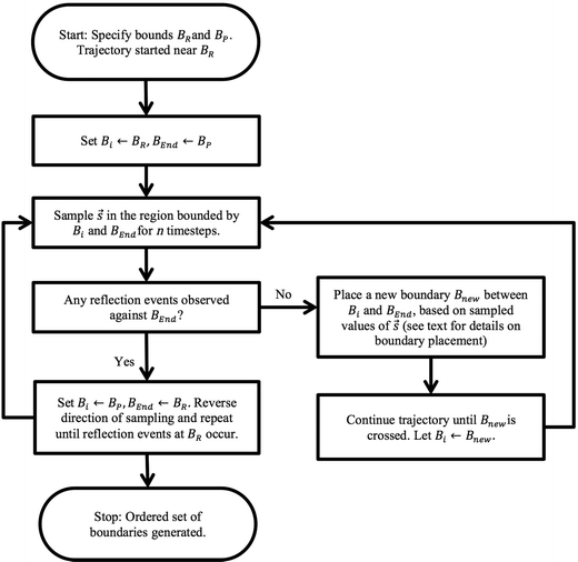
The overall adaptive BXD procedure is illustrated by the flowchart in Fig. 3, which assumes that the adaptive procedure has been initialised near BR, so that the first pass involves generating boundaries en route to BP. At the start of the trajectory, Bi ← BR, and BEnd ← BP (i.e., Bi and BEnd initially enclose the region Γ ≡ Γ2, with Γ1 = 0). After n steps of dynamics, sampling ![[s with combining right harpoon above (vector)]](https://www.rsc.org/images/entities/i_char_0073_20d1.gif) within Γ2 (constrained through application of the BXD velocity reflection procedure), there are two possible outcomes: (1) velocity reflections against BEnd were observed, implying that the path from Bi to BEnd requires no additional acceleration, or (2) velocity reflections against BEnd were not observed, which means that an additional bound Bnew is required according to the procedure outlined below in section 2.4.2. Dynamics are then run until the system crosses Bnew, at which point Bi ← Bnew. The dynamics in this hitherto unexplored space are then restricted in the region of Γ2 through the application of the BXD velocity reflection procedure. The sampling procedure is repeated until the dynamics reach BEnd, at which point Bi ← BP and BEnd ← BR, and the dynamics sweep back for a second pass in the opposite direction. Upon completion of the reverse pass, the Fig. 3 schematic arrives at the “Stop” point, and Γ will have been partitioned into a set of boxes with bounds BR, B1, B2, …, Bn, BP for subsequent use in BXD runs to generate free energy surfaces to a specified degree of convergence.
within Γ2 (constrained through application of the BXD velocity reflection procedure), there are two possible outcomes: (1) velocity reflections against BEnd were observed, implying that the path from Bi to BEnd requires no additional acceleration, or (2) velocity reflections against BEnd were not observed, which means that an additional bound Bnew is required according to the procedure outlined below in section 2.4.2. Dynamics are then run until the system crosses Bnew, at which point Bi ← Bnew. The dynamics in this hitherto unexplored space are then restricted in the region of Γ2 through the application of the BXD velocity reflection procedure. The sampling procedure is repeated until the dynamics reach BEnd, at which point Bi ← BP and BEnd ← BR, and the dynamics sweep back for a second pass in the opposite direction. Upon completion of the reverse pass, the Fig. 3 schematic arrives at the “Stop” point, and Γ will have been partitioned into a set of boxes with bounds BR, B1, B2, …, Bn, BP for subsequent use in BXD runs to generate free energy surfaces to a specified degree of convergence.
![[Doublestruck R]](https://www.rsc.org/images/entities/char_e175.gif) n×M be the set of the sampled values of
n×M be the set of the sampled values of ![[s with combining right harpoon above (vector)]](https://www.rsc.org/images/entities/i_char_0073_20d1.gif) , illustrated as blue circles in Fig. 4A, and let
, illustrated as blue circles in Fig. 4A, and let ![[R with combining right harpoon above (vector)]](https://www.rsc.org/images/entities/i_char_0052_20d1.gif) ∈
∈ ![[Doublestruck R]](https://www.rsc.org/images/entities/char_e175.gif) n be the vector of distances r from Bi to each sampled value
n be the vector of distances r from Bi to each sampled value ![[s with combining right harpoon above (vector)]](https://www.rsc.org/images/entities/i_char_0073_20d1.gif) in S. The vector
in S. The vector ![[R with combining right harpoon above (vector)]](https://www.rsc.org/images/entities/i_char_0052_20d1.gif) provides information on how far from Bi the next boundary should be placed, the location of which is determined as follows:
provides information on how far from Bi the next boundary should be placed, the location of which is determined as follows:
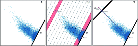 | ||
Fig. 4 Illustration of the adaptive boundary generation procedure. Panel A shows sampling of values within a 2d collective variable space, with an existing boundary Bi; panel B shows histogram binning of the distances with respect to the existing boundary Bi. ![[s with combining right harpoon above (vector)]](https://www.rsc.org/images/entities/i_char_0073_20d1.gif) min and min and![[s with combining right harpoon above (vector)]](https://www.rsc.org/images/entities/i_char_0073_20d1.gif) max, located within histogram bins bmin and bmax, are both shaded in red. Panel C shows generation of a new bound Bnew, where the norm defined in eqn (14) is illustrated by the purple arrow. max, located within histogram bins bmin and bmax, are both shaded in red. Panel C shows generation of a new bound Bnew, where the norm defined in eqn (14) is illustrated by the purple arrow. | ||
(1) A normalized histogram of ![[R with combining right harpoon above (vector)]](https://www.rsc.org/images/entities/i_char_0052_20d1.gif) is computed to give p(r), a probability density function representing the distances from Bi that a trajectory samples between reflections, as shown in Fig. 4B.
is computed to give p(r), a probability density function representing the distances from Bi that a trajectory samples between reflections, as shown in Fig. 4B.
(2) From p(r), we calculate the cumulative distribution function  . We then identify a histogram bin bmax in p(r) with a bin centre rmax chosen so that P(rmax) ≥ (1 − ε). ε ∈ (0, 1) is a parameter which specifies the “probability threshold” at which to place a new boundary (the value of ε is specified by the user, and typically ranges from 0.01–0.1). We then identify
 ![[s with combining right harpoon above (vector)]](https://www.rsc.org/images/entities/i_char_0073_20d1.gif) max (the mean value of the sampled values in S that fall within bin bmax), illustrated in Fig. 4B, as the point at which to place a new boundary Bnew.
max (the mean value of the sampled values in S that fall within bin bmax), illustrated in Fig. 4B, as the point at which to place a new boundary Bnew.
(3) To determine the orientation of Bnew as an (M − 1)-dimensional plane, we use a simple strategy consistent with BXD's origins in transition state theory (TST) – i.e., Bnew should be more or less orthogonal to the path of the observed dynamics.13,14 With bmin defined as the first bin in the histogram of ![[R with combining right harpoon above (vector)]](https://www.rsc.org/images/entities/i_char_0052_20d1.gif) (see Fig. 4B), we calculate
(see Fig. 4B), we calculate ![[s with combining right harpoon above (vector)]](https://www.rsc.org/images/entities/i_char_0073_20d1.gif) min (the mean value of the sampled values in S that fall within bmin). With this definition,
min (the mean value of the sampled values in S that fall within bmin). With this definition, ![[s with combining right harpoon above (vector)]](https://www.rsc.org/images/entities/i_char_0073_20d1.gif) min represents the average value of
min represents the average value of ![[s with combining right harpoon above (vector)]](https://www.rsc.org/images/entities/i_char_0073_20d1.gif) immediately prior to and after reflection against Bi, i.e. the mean crossing point through Bi. Similarly,
immediately prior to and after reflection against Bi, i.e. the mean crossing point through Bi. Similarly, ![[s with combining right harpoon above (vector)]](https://www.rsc.org/images/entities/i_char_0073_20d1.gif) max represents the average crossing point through Bnew. The vector from
max represents the average crossing point through Bnew. The vector from ![[s with combining right harpoon above (vector)]](https://www.rsc.org/images/entities/i_char_0073_20d1.gif) min to
min to ![[s with combining right harpoon above (vector)]](https://www.rsc.org/images/entities/i_char_0073_20d1.gif) max thus serves as an approximate dynamical pathway through the box, and we define the unit norm for Bnew as
max thus serves as an approximate dynamical pathway through the box, and we define the unit norm for Bnew as
 | (14) |
The unit norm in eqn (14), combined with ![[s with combining right harpoon above (vector)]](https://www.rsc.org/images/entities/i_char_0073_20d1.gif) max, allow us to fully define the new boundary Bnew, as illustrated in Fig. 4C. The next time the trajectory crosses Bnew, it becomes enforced as a constraint (i.e., Bi ← Bnew), and an identical analysis will be carried out to determine the next Bnew.
max, allow us to fully define the new boundary Bnew, as illustrated in Fig. 4C. The next time the trajectory crosses Bnew, it becomes enforced as a constraint (i.e., Bi ← Bnew), and an identical analysis will be carried out to determine the next Bnew.
As discussed above, adaptive boundary generation in this fashion will eventually lead to reflection against BP. Once a trajectory reaches the barrier via adaptive boundary generation on the reactant side of the barrier, reflection against BP generally follows rapidly without any need for boundaries on the product side of the barrier. To generate boundaries on the product side, a second adaptive sweep from BP to BR is required. To do this, the direction of sampling is reversed, and the adaptive boundary generation process is repeated going the opposite way. The only difference is that – because adaptive boundaries are already in place on the reactant side of the barrier – the reactant region is unlikely to require any more boundaries on the second sweep. For example, consider a BXD trajectory on its second sweep which is passing through the reactant region enclosed by boundaries Bi and Bi−1 (both of which were adaptively generated in the first pass). It is likely for reflection events against Bi−1 to be observed – i.e., sampling within this region is already suitably accelerated by BXD, and the trajectory can move on to the region defined by boundaries Bi−1 and Bi−2. Should we observe that the trajectory has not inverted against Bi−1 after n steps, then an additional boundary is adaptively generated as described above.
3 Multidimensional adaptive sampling of chemical reactions in liquids
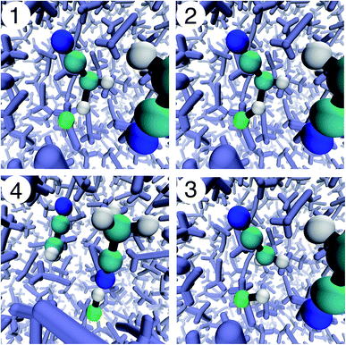
As an initial test of the multidimensional adaptive BXD scheme outlined above, we investigated F + CD3CN → DF + CD2CN in CD3CN solvent. This system has recently been the subject of both ultrafast transient IR spectroscopy experiments and corresponding non-equilibrium MD simulations.63,64 As such, it provides an excellent test case for investigating the algorithms described above, and also for evaluating their performance and accuracy. The reaction, which takes place in deuterated acetonitrile solvent (CD3CN), consists of deuterium abstraction from acetonitrile by the fluorine atom, snapshots of which are illustrated in Fig. 5. Reactive molecular dynamics are possible using a customized version of the CHARMM molecular dynamics software suite, using a parallel implementation of the multi-state empirical valence bond (MS-EVB) method. The simulation includes a single F radical embedded in a periodic box of 62 CD3CN solvent molecules. With a total of 64 MS-EVB states parallelized across 64 CPU cores, our simulations are able to treat the reactive process leading to DF as well as transient deuterium transfer from the nascent DF to the nitrile group on the other solvent molecules.64 The MS-EVB coupling elements were fit to explicitly correlated CCSD(T)-F12 electronic structure theory extrapolated to the infinite basis set limit (the contours of this PES are shown in Fig. 6). This procedure yields an accurate reactive PES, which is critical to understanding non-equilibrium energy deposition for reactions of this sort.A one-dimensional implementation of BXD was previously used in these simulations to restrict the distance between the F radical and the reactive deuterium between 1.5 Å and 1.8 Å. This prevented the F radical diffusing away from its co-reactant during pre-production equilibration sampling runs. In the production NVE runs, the lower bound was removed. This allowed the reaction to occur, so that we could obtain an accurate measurement of energy deposition and relaxation in the nascent reaction products. At the time these studies were published, it was not possible to use BXD to generate a free energy surface for this reaction given that reversible reactive sampling requires the use of at least two CVs: the distance between the F radical and deuterium (F–D distance), and the distance between transferring deuterium and the carbon atom to which it is bonded (C–D distance). Constraint of the F–D distance accelerates abstraction over a relatively early barrier, and constraint of the C–D distance prevents the product DF from immediately diffusing away from its co-product. In addition to BXD sampling of the condensed phase reaction, we also carried out BXD sampling of the gas phase reaction, which included only three EVB states: the reactant F + CD3CN state, the co-product DF + CD2CN state, and the [CD3CND]+⋯[F]− state. Unless stated otherwise, all the results presented herein were run with a time step of 0.1 fs, using a Langevin thermostat at 300 K with a friction coefficient of 20 ps−1.
3.1 Adaptively generated BXD boundaries along the F + CD3CN reaction path
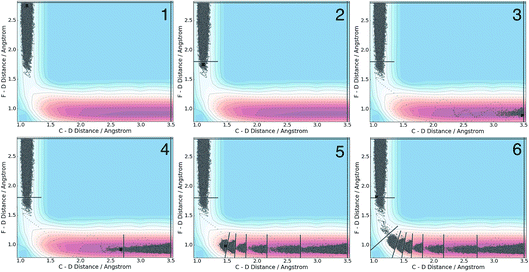
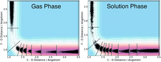
We applied the adaptive boundary generation procedure described in section 2.4 to sample this reaction and create BXD boundaries that could be used to accelerate the calculation of a free energy surface. This constitutes an interesting and particularly stringent test of our adaptive BXD procedure because of the large change in gradients along the reaction pathway: the gradients on the reactant side of the TS are very flat, while those on the product side are very steep. Application of adaptive BXD to this system also enables us to comment on an outstanding experimental question – namely, to what extent does the free energy surface of the gas phase chemical reaction resemble the free energy surface of the reaction in a strongly coupled solvent like CD3CN? In the gas phase, the 0 K reaction enthalpy is −37 kcal mol−1, most of which is potentially available for deposition into the nascent DF product. Measurements carried out using ultrafast transient IR spectroscopy in solution showed deposition of substantial vibrational energy (i.e., at least v = 2) in the stretching motion of the nascent DF product for the reaction taking place in solution. This value places a firm lower limit on exothermicity of the reaction free energy; however, a detailed analysis of the free energy profiles in both the gas phase and in solvent is beyond experimental reach.As outlined above, adaptive BXD free energy sampling was undertaken in a CV space comprised of the F–D and C–D distances: an F–D distance of 2.7 Å was used to define BR, and a C–D distance of 3.5 Å was used to define BP. Adaptive sampling times of 100 ps (in the gas phase) and 30 ps (in solution phase) per box were used to determine the placement of new boundaries, with ε = 0.01 (guaranteeing that new boundaries are placed at a location visited no more than 1% of the time). Fig. 6 shows a series of snapshots taken during the automated boundary location procedure, illustrating how the adaptive algorithm works. Beginning from an initial point sampled near BR, BXD adaptively generates a boundary, which allows it to sample regions near the TS. Once the dynamics arrive at the TS, the system rapidly descends toward products, and quickly arrives at BP. At this point, BXD begins sweeping back in the opposite direction, adaptively generating boundaries which eventually return it back to the first box bounded by BR. Fig. 7 shows the final set of adaptively generated boundaries used to sample the free energy along the reaction pathway in both solution phase and in the gas phase. The plots also show the dynamical traces in CV space used to construct the BXD boundaries. There are some important points to note with respect to Fig. 6 and 7: (1) the adaptively generated boundaries generally follow the route taken by the dynamics along the reaction pathway, with orientations that are roughly orthogonal to the dynamical pathway through CV space; (2) the spacing between boundaries varies as a function of the steepness of the free energy surface (the gradient) of the underlying PES and the corresponding free energy profile – i.e., steep regions with large gradients require several boundaries, whereas less steep regions with smaller gradients require fewer boundaries; and (3) the reaction pathway in solvent has more adaptively generated BXD boundaries than the corresponding gas phase pathway, as a result of solvent friction effects that do not occur in the gas phase. Placing such a large number of BXD boundaries by user trial and error would be an extremely labour intensive process.
3.2 Free energy sampling within the adaptive boundaries
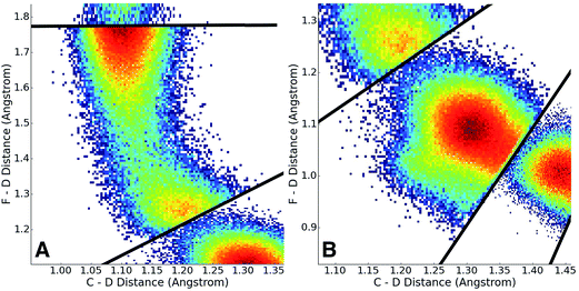
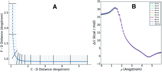
Having adaptively generated boundaries for both the solution and gas phase reactions, the standard BXD sampling procedure could then be applied. For the gas phase, the system is small enough that it was possible to gather all the required statistics with a single 100 ns trajectory, where the trajectory was sequentially restrained within each box until 100 reflection events had occurred on either side of the boundary before being allowed through to the next box (another way of deciding how long to remain in the box is to monitor the point at which the MFPT reaches a user-specified convergence criterion). Given the larger size of the solution phase system along with the increased computational requirements that result from the 64 EVB states, we exploited the trivial parallelism of BXD to run trajectories in each box until meeting a user-specified convergence criterion (i.e., that the box-to-box MFPTs did not change by more than 0.1% with increased sampling), giving a total of 12 ns of dynamics across all boxes. Fig. 8 shows examples of the sampled values of the CVs obtained in the solution phase simulations, and demonstrates the sort of statistics obtained in two different regions along the free energy profile: (A) in the vicinity of the transition state, and (B) along a steep ‘post-transition’ state region after DF has formed.Once sampling was completed within each box (generating statistics similar to those shown in Fig. 7), MFPTs were calculated as described in section 2.1, and the results used to generate a ‘box-averaged’ free energy profile and corresponding ‘box-averaged’ probability spanning BR to BP. A higher-resolution free energy profile was obtained placing the statistics for a particular box into histogram bins and then using eqn (4) to renormalize by the box-averaged probabilities. Fig. 9A shows the smaller histogram bins into which we partitioned the statistics in each box to accomplish this. In the 1d case, high-resolution partitioning along the dynamical pathway is straightforward; in this case (and more generally for higher-dimensional cases), our strategy is as follows:
(1) Define a path ρ which passes through the average dynamical crossing points through each boundary (i.e., ![[s with combining right harpoon above (vector)]](https://www.rsc.org/images/entities/i_char_0073_20d1.gif) max), and spans BR to BP.
max), and spans BR to BP.
(2) Each region between a set of boundaries is then partitioned into a series of bisecting hyperplanes, to an arbitrary user-specified resolution. The regions between these bisecting hyperplanes constitute the high-resolution histogram bins. The centre of each bin is chosen to be the point along ρ which is equidistant from the hyperplanes that bound the bin.
The blue line in Fig. 9A shows the path ρ which spans BR to BP, and which was used to generate finer histogram bins for plotting the high-resolution free energy profile. Fig. 9B shows the corresponding high-resolution BXD free energy profiles for the gas phase reaction. The overlapping curves in this plot show how the free energy profiles change with increasing sampling time, giving some indication of how quickly the BXD free energy profile converges in this particular system.
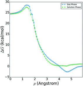
Fig. 10 shows a comparison of the reactive free energy surfaces obtained in both the gas phase and in solvent. In the vicinity of the reactants and transition states, the profiles are very similar; however, they show considerable differences in the post-reaction region. The reason for this difference arises from post-reaction hydrogen bonding complexes formed by the nascent DF. In the gas phase BXD free energy sampling, the DF rotates around the backside of its CD2CN co-product and finds a stable hydrogen-bonding complex with the nitrile moiety. In solvent, such interactions are possible with any of a wide range of nearby solvent molecules, and therefore no distinct minima can be observed along the free energy profile. In terms of understanding the DF energy deposition observed in the previously published experimental and MD results, the key quantity in Fig. 10 is the free energy difference between: (1) the maximum value observed near the transition state region, and (2) the minimum observed near the product state region. This quantity places an upper bound on the amount of energy which may be deposited into the nascent DF: for the reaction taking place in solvent the value is 27.6 kcal mol−1, and for the reaction taking place in the gas phase the value is 31.1 kcal mol−1. Both of these values are in good agreement with previous experimental and modelling studies. Our previously published experimental and MD studies indicated the prompt deposition of ∼23 kcal mol−1 into the stretching motion of the nascent DF prior to relaxation.63,64 While gas phase experiments of F + CD3CN are not available for direct comparison to our free energy results, experiments examining gas-phase energy deposition into HF in the F + CH3CN reaction have been performed,65 and suggest that the nascent diatomic product in solvent contains slightly less excitation than in the gas phase.63 This is consistent with the results in Fig. 10, which indicate that more energy is available to the products in the gas phase reaction than in the solvent reaction.
4 Conclusions
In this paper, we have outlined an adaptive and automated procedure for generating boundaries in a multi-dimensional space of CVs. Our automated algorithm reduces the user effort required to carry out both rare event and free energy sampling in both one-dimensional and multi-dimensional cases; it generates box boundaries which are far enough apart to avoid any problems related to dynamical decorrelation, but which afford optimal acceleration. The extension of BXD to multidimensional collective variables provides an effective way to sample increasingly complex systems, but retains much of the simplicity and original properties of the 1-dimensional BXD implementation. The adaptive BXD scheme tested in this paper has been implemented in CHARMM, and will soon be available in the release version (we have also made initial efforts toward a BXD implementation in the TeraChem66ab initio dynamics package). The tests reported in this paper were carried out using the CHARMM implementation, in conjunction with parallelizable MS-EVB machinery also available in CHARMM.64 This framework allowed us to map free energy along a deuterium abstraction reaction pathway in both gas and solution phases. The results we obtained are in agreement with previously published experimental and modelling studies, providing good evidence for the reliability of our adaptive multidimensional BXD implementation.We believe that the adaptive scheme outlined in this paper, which allows us to generate hyperplanes in multi-dimensional collective variable space, may be more broadly useful to a wide range of techniques which rely on splicing up configuration space into a set of interfaces or boundaries. In the future, we will explore rigorous methods for estimating the error bars of free energy surfaces generated using BXD.67 We also plan to explore extensions of the adaptive BXD scheme in systems with CV spaces that have dimensionalities of three and higher – e.g., enzyme reactions and conformational dynamics,68 drug binding,69 and chemical reactions at surfaces and in liquids.70 As shown in eqn (7), implementation of BXD in multi-dimensional CV space requires definitions of the gradient in CV space, ∇ϕ, a wide library of which are available in the PLUMED71 package. We are presently working on writing the BXD algorithm as a portable, and mostly ‘standalone’ plugin that may be easily interfaced with a wide range of molecular dynamics packages, a similar philosophy to that which has been adopted by PLUMED.71 Implementation of adaptive BXD in a package of this sort should allow it to be used in a wide range of contexts.
5 Appendix: velocity reflection in two-dimensional CV space
In this section we give details on the calculations required to perform velocity reflection for a simple but illustrative case. Consider a system of atoms A, B and C where our collective variables are the distances AB and BC. This style of collective variable is useful in many situations, including the acceleration of abstraction reactions as discussed in the main document.For the sake of brevity we restrict ourselves to 2 spatial coordinates. Let ![[r with combining right harpoon above (vector)]](https://www.rsc.org/images/entities/i_char_0072_20d1.gif) = [ax, ay, bx, by, cx, cy] be the coordinates and
= [ax, ay, bx, by, cx, cy] be the coordinates and ![[v with combining right harpoon above (vector)]](https://www.rsc.org/images/entities/i_char_0076_20d1.gif) = [Vxa, Vya, Vxb, Vyb, Vxc, Vyc] be the velocities of atoms A, B and C, and let M be the diagonal matrix of atomic masses, i.e.:
= [Vxa, Vya, Vxb, Vyb, Vxc, Vyc] be the velocities of atoms A, B and C, and let M be the diagonal matrix of atomic masses, i.e.:
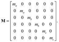 | (A.1) |
Our collective variable s(![[r with combining right harpoon above (vector)]](https://www.rsc.org/images/entities/i_char_0072_20d1.gif) ) is given by:
) is given by:
 | (A.2) |
Suppose we have some BXD boundary B, defined as a two-dimensional line in Hessian form with norm ![[n with combining circumflex]](https://www.rsc.org/images/entities/i_char_006e_0302.gif) = (n1, n2) and point D. The constraint on our dynamics is
= (n1, n2) and point D. The constraint on our dynamics is
| ϕ ≡ n1rAB + n2rBC + D ≥ 0. | (A.3) |
Suppose that we identify a timestep in which our constraint will no longer be satisfied – i.e., the stepping forward using the current velocities will result in a boundary being crossed, and we require a velocity reflection. In order to perform the velocity reflection using a Lagrangian multiplier, we need to compute ∇ϕ, the transpose of which is given by
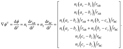 | (A.4) |
The expression above demonstrates how it is simple to construct the reflection procedure from the gradients of the individual collective variables. With ∇ϕ in hand, it is a simple matter to determine the Lagrangian multiplier λ with which the velocities may be inverted. From eqn (12) we may compute λ via
 | (A.5) |
![[v with combining right harpoon above (vector)]](https://www.rsc.org/images/entities/i_char_0076_20d1.gif) ′(t) =
′(t) = ![[v with combining right harpoon above (vector)]](https://www.rsc.org/images/entities/i_char_0076_20d1.gif) (t) + λM−1∇ϕT. In the resulting velocities, the components normal to the boundary are inverted, and thus the constraint is satisfied.
(t) + λM−1∇ϕT. In the resulting velocities, the components normal to the boundary are inverted, and thus the constraint is satisfied.
Acknowledgements
DRG acknowledges funding as a Royal Society research fellow. MOC acknowledges funding for a PhD studentship from EPSRC. Dmitry Shalashilin, Jeremy Harvey, and Andrew Orr-Ewing provided useful comments along the way.References
- J.-H. Prinz, et al., Markov models of molecular kinetics: generation and validation, J. Chem. Phys., 2011, 134(17), 174105 CrossRef PubMed.
- L. Vereecken, D. R. Glowacki and M. J. Pilling, Theoretical chemical kinetics in tropospheric chemistry: methodologies and applications, Chem. Rev., 2015, 115(10), 4063–4114 CrossRef CAS PubMed.
- D. R. Glowacki and M. J. Pilling, Unimolecular reactions of peroxy radicals in atmospheric chemistry and combustion, ChemPhysChem, 2010, 11(18), 3836–3843 CrossRef CAS PubMed.
- D. R. Glowacki, et al., MESMER: an open-source master equation solver for multi-energy well reactions, J. Phys. Chem. A, 2012, 116(38), 9545–9560 CrossRef CAS PubMed.
- S. Maeda, K. Ohno and K. Morokuma, Systematic exploration of the mechanism of chemical reactions: the global reaction route mapping (GRRM) strategy using the ADDF and AFIR methods, Phys. Chem. Chem. Phys., 2013, 15(11), 3683–3701 RSC.
- Y. Fang, et al., Communication: real time observation of unimolecular decay of Criegee intermediates to OH radical products, J. Chem. Phys., 2016, 144(6), 061102 CrossRef PubMed.
- L. Y. Luk, et al., Unraveling the role of protein dynamics in dihydrofolate reductase catalysis, Proc. Natl. Acad. Sci. U. S. A., 2013, 110(41), 16344–16349 CrossRef CAS PubMed.
- J. L. Skinner and P. G. Wolynes, Relaxation processes and chemical kinetics, J. Chem. Phys., 1978, 69(5), 2143–2150 CrossRef CAS.
- D. Chandler, Statistical mechanics of isomerization dynamics in liquids and the transition state approximation, J. Chem. Phys., 1978, 68(6), 2959–2970 CrossRef CAS.
- B. Berger and T. Leighton, Protein folding in the hydrophobic-hydrophilic (HP) is NP-complete, J. Comput. Biol., 2009, 5(1), 27–40 CrossRef PubMed.
- W. E. Hart and S. Istrail, Robust proofs of NP-hardness for protein folding: general lattices and energy potentials, J. Comput. Biol., 1997, 1–22 CrossRef CAS PubMed.
- I. Kassal, et al., Simulating Chemistry Using Quantum Computers, Annu. Rev. Phys. Chem., 2011, 185–207 CrossRef CAS PubMed.
- D. R. Glowacki, E. Paci and D. V. Shalashilin, Boxed Molecular Dynamics: A Simple and General Technique for Accelerating Rare Event Kinetics and Mapping Free Energy in Large Molecular Systems, J. Phys. Chem. B, 2009, 113(52), 16603–16611 CrossRef CAS PubMed.
- D. R. Glowacki, E. Paci and D. V. Shalashilin, Boxed Molecular Dynamics: Decorrelation Time Scales and the Kinetic Master Equation, J. Chem. Theory Comput., 2011, 7(5), 1244–1252 CrossRef CAS PubMed.
- D. V. Shalashilin, et al., Peptide kinetics from picoseconds to microseconds using boxed molecular dynamics: power law rate coefficients in cyclization reactions, J. Chem. Phys., 2012, 137(16), 9 CrossRef PubMed.
- J. Booth, et al., Recent applications of boxed molecular dynamics: a simple multiscale technique for atomistic simulations, Philos. Trans. R. Soc., A, 2014, 372(2021), 13 CrossRef PubMed.
- B. Fačkovec, E. Vanden-Eijnden and D. J. Wales, Markov state modeling and dynamical coarse-graining via discrete relaxation path sampling, J. Chem. Phys., 2015, 143(4), 044119 CrossRef PubMed.
- G. T. Dunning, D. R. Glowacki, T. J. Preston, S. J. Greaves, G. M. Greetham, I. P. Clark, M. Towrie, J. N. Harvey and A. J. Orr-Ewing, Vibrational relaxation and micro-solvation of DF following F-atom reactions in polar solvents, Science, 2015, 347(6221), 530–533 CrossRef CAS PubMed.
- D. R. Glowacki, A. J. Orr-Ewing and J. N. Harvey, Product energy deposition of CN + alkane H abstraction reactions in gas and solution phases, J. Chem. Phys., 2011, 134(21), 214508 CrossRef PubMed.
- D. R. Glowacki, A. J. Orr-Ewing and J. N. Harvey, A parallel multistate framework for atomistic non-equilibrium reaction dynamics of solutes in strongly interacting organic solvents, arXiv:1412.4180, 2014.
- D. R. Glowacki, et al., Ultrafast energy flow in the wake of solution-phase bimolecular reactions, Nat. Chem., 2011, 3(11), 850–855 CrossRef CAS PubMed.
- S. J. Greaves, et al., Vibrationally Quantum-State-Specific Reaction Dynamics of H Atom Abstraction by CN Radical in Solution, Science, 2011, 331(6023), 1423–1426 CrossRef CAS PubMed.
- J. J. Nogueira, et al., Unraveling the Factors That Control Soft Landing of Small Silyl Ions on Fluorinated Self-Assembled Monolayers, J. Phys. Chem. C, 2014, 118(19), 10159–10169 CAS.
- R. A. Rose, et al., Reaction dynamics of CN radicals with tetrahydrofuran in liquid solutions, Phys. Chem. Chem. Phys., 2012, 14(30), 10424–10437 RSC.
- E. S. Savoy and F. A. Escobedo, Molecular Simulations of Wetting of a Rough Surface by an Oily Fluid: Effect of Topology, Chemistry, and Droplet Size on Wetting Transition Rates, Langmuir, 2012, 28(7), 3412–3419 CrossRef CAS PubMed.
- E. S. Savoy and F. A. Escobedo, Simulation Study of Free-Energy Barriers in the Wetting Transition of an Oily Fluid on a Rough Surface with Reentrant Geometry, Langmuir, 2012, 28(46), 16080–16090 CrossRef CAS PubMed.
- S. L. Meadley and F. A. Escobedo, Thermodynamics and kinetics of bubble nucleation: simulation methodology, J. Chem. Phys., 2012, 137(7), 074109 CrossRef PubMed.
- A. J. Orr-Ewing, et al., Chemical Reaction Dynamics in Liquid Solutions, J. Phys. Chem. Lett., 2011, 2(10), 1139–1144 CrossRef CAS PubMed.
- J. J. Booth and D. V. Shalashilin, Fully Atomistic Simulations of Protein Unfolding in Low Speed Atomic Force Microscope and Force Clamp Experiments with the Help of Boxed Molecular Dynamics, J. Phys. Chem. B, 2016, 120(4), 700–708 CrossRef CAS PubMed.
- A. J. Orr-Ewing, Perspective: bimolecular chemical reaction dynamics in liquids, J. Chem. Phys., 2014, 140(9), 090901 CrossRef PubMed.
- A. K. Faradjian and R. Elber, Computing time scales from reaction coordinates by milestoning, J. Chem. Phys., 2004, 120, 10880–10889 CrossRef CAS PubMed.
- E. Vanden-Eijnden and M. Venturoli, Markovian milestoning with Voronoi tessellations, J. Chem. Phys., 2009, 130, 194101 CrossRef PubMed.
- R. J. Allen, D. Frenkel and P. R. ten Wolde, Simulating rare events in equilibrium or nonequilibrium stochastic systems, J. Chem. Phys., 2006, 124(2), 024102 CrossRef PubMed.
- R. J. Allen, P. B. Warren and P. R. ten Wolde, Sampling Rare Switching Events in Biochemical Networks, Phys. Rev. Lett., 2005, 94(1), 018104 CrossRef PubMed.
- T. S. van Erp, D. Moroni and P. G. Bolhuis, A novel path sampling method for the calculation of rate constants, J. Chem. Phys., 2003, 118(17), 7762–7774 CrossRef CAS.
- A. Warmflash, P. Bhimalapuram and A. R. Dinner, Umbrella sampling for nonequilibrium processes, J. Chem. Phys., 2007, 127(15), 154112 CrossRef PubMed.
- J. Juraszek, et al., Efficient Numerical Reconstruction of Protein Folding Kinetics with Partial Path Sampling and Pathlike Variables, Phys. Rev. Lett., 2013, 110(10), 108106 CrossRef CAS PubMed.
- V. Thapar and F. A. Escobedo, Simultaneous estimation of free energies and rates using forward flux sampling and mean first passage times, J. Chem. Phys., 2015, 143(24), 244113 CrossRef PubMed.
- D. Bhatt and I. Bahar, An adaptive weighted ensemble procedure for efficient computation of free energies and first passage rates, J. Chem. Phys., 2012, 137(10), 104101 CrossRef PubMed.
- G. M. Torrie and J. P. Valleau, Nonphysical sampling distributions in Monte Carlo free-energy estimation: Umbrella sampling, J. Comput. Phys., 1977, 23(2), 187–199 CrossRef.
- B. M. Dickson, D. E. Makarov and G. Henkelman, Pitfalls of choosing an order parameter for rare event calculations, J. Chem. Phys., 2009, 131(7), 074108 CrossRef PubMed.
- S. V. Krivov, On Reaction Coordinate Optimality, J. Chem. Theory Comput., 2013, 9(1), 135–146 CrossRef CAS PubMed.
- B. R. Brooks, et al., CHARMM: the biomolecular simulation program, J. Comput. Chem., 2009, 30(10), 1545–1614 CrossRef CAS PubMed.
- C. Bartels and M. Karplus, Multidimensional adaptive umbrella sampling: applications to main chain and side chain peptide conformations, J. Comput. Chem., 1997, 18(12), 1450–1462 CrossRef CAS.
- M. Mezei, Adaptive umbrella sampling: self-consistent determination of the non-Boltzmann bias, J. Comput. Phys., 1987, 68(1), 237–248 CrossRef.
- J. Comer, et al., The Adaptive Biasing Force Method: Everything You Always Wanted To Know but Were Afraid To Ask, J. Phys. Chem. B, 2015, 119(3), 1129–1151 CrossRef CAS PubMed.
- W.-N. Du and P. G. Bolhuis, Adaptive single replica multiple state transition interface sampling, J. Chem. Phys., 2013, 139(4), 044105 CrossRef PubMed.
- L. C. T. Pierce, et al., Accelerating chemical reactions: exploring reactive free-energy surfaces using accelerated ab initio molecular dynamics, J. Chem. Phys., 2011, 134(17), 174107 CrossRef PubMed.
- L. Alessandro and L. G. Francesco, Metadynamics: a method to simulate rare events and reconstruct the free energy in biophysics, chemistry and material science, Rep. Prog. Phys., 2008, 71(12), 126601 CrossRef.
- G. Bussi, A. Laio and M. Parrinello, Equilibrium Free Energies from Nonequilibrium Metadynamics, Phys. Rev. Lett., 2006, 96(9), 090601 CrossRef PubMed.
- G. Ozer, et al., Adaptive Steered Molecular Dynamics of the Long-Distance Unfolding of Neuropeptide Y, J. Chem. Theory Comput., 2010, 6(10), 3026–3038 CrossRef CAS PubMed.
- Y. Guo, et al., Intramolecular dynamics diffusion theory approach to complex unimolecular reactions, J. Chem. Phys., 1999, 110(12), 5521–5525 CrossRef CAS.
- Y. Guo, et al., Predicting nonstatistical unimolecular reaction rates using Kramers' theory, J. Chem. Phys., 1999, 110(12), 5514–5520 CrossRef CAS.
- E. Martinez-Nunez and D. V. Shalashilin, Acceleration of Classical Mechanics by Phase Space Constraints, J. Chem. Theory Comput., 2006, 2(4), 912–919 CrossRef CAS PubMed.
- D. V. Shalashilin and D. L. Thompson, Monte Carlo Variational Transition-State Theory Study of the Unimolecular Dissociation of RDX, J. Phys. Chem. A, 1997, 101(5), 961–966 CrossRef CAS.
- D. V. Shalashilin and D. L. Thompson, Method for predicting IVR-limited unimolecular reaction rate coefficients, J. Chem. Phys., 1997, 107(16), 6204–6212 CrossRef CAS.
- D. R. Glowacki, E. Paci and D. V. Shalashilin, Boxed molecular dynamics: a simple and general technique for accelerating rare event kinetics and mapping free energy in large molecular systems, J. Phys. Chem. B, 2009, 113(52), 16603–16611 CrossRef CAS PubMed.
- R. Featherstone, Rigid body dynamics algorithms, 2014 Search PubMed.
- J.-P. Ryckaert, G. Ciccotti and H. J. C. Berendsen, Numerical integration of the Cartesian equations of motion of a system with constraints: molecular dynamics of n-alkanes, J. Comput. Phys., 1977, 23, 327–341 CrossRef CAS.
- H. C. Andersen, Rattle: a “velocity” version of the shake algorithm for molecular dynamics calculations, J. Comput. Phys., 1983, 52, 24–34 CrossRef CAS.
- P. Lötstedt, Numerical Simulation of Time-Dependent Contact and Friction Problems in Rigid Body Mechanics, SIAM J. Sci. Comput., 1984, 5, 370–393 CrossRef.
- P. Lötstedt, Mechanical Systems of Rigid Bodies Subject to Unilateral Constraints, SIAM J. Appl. Math., 1982, 42, 281–296 CrossRef.
- G. T. Dunning, et al., Vibrational relaxation and microsolvation of DF after F-atom reactions in polar solvents, Science, 2015, 347, 530–533 CrossRef CAS PubMed.
- D. R. Glowacki, A. J. Orr-Ewing and J. N. Harvey, Non-equilibrium reaction and relaxation dynamics in a strongly interacting explicit solvent: F + CD3CN treated with a parallel multi-state EVB model, J. Chem. Phys., 2015, 143, 044120 CrossRef PubMed.
- K. Dehe and H. Heydtmann, HF infrared emission from the reactions of atomic fluorine with methylcyanide, methylisocyanide, dimethylsulfide and dimethyldisulfide, Chem. Phys. Lett., 1996, 262(6), 683–688 CrossRef CAS.
- I. S. Ufimtsev and T. J. Martínez, Graphical processing units for quantum chemistry, Comput. Sci. Eng., 2008, 10(6), 26–34 CrossRef CAS.
- D. M. Zuckerman and T. B. Woolf, Theory of a Systematic Computational Error in Free Energy Differences, Phys. Rev. Lett., 2002, 89(18), 180602 CrossRef PubMed.
- D. R. Glowacki, J. N. Harvey and A. J. Mulholland, Taking Ockham's razor to enzyme dynamics and catalysis, Nat. Chem., 2012, 4(3), 169–176 CrossRef CAS PubMed.
- M. De Vivo, et al., Role of Molecular Dynamics and Related Methods in Drug Discovery, J. Med. Chem., 2016, 59(9), 4035–4061 CrossRef CAS PubMed.
- B. K. Carpenter, J. N. Harvey and A. J. Orr-Ewing, The Study of Reactive Intermediates in Condensed Phases, J. Am. Chem. Soc., 2016, 138(14), 4695–4705 CrossRef CAS PubMed.
- M. Bonomi, et al., PLUMED: a portable plugin for free-energy calculations with molecular dynamics, Comput. Phys. Commun., 2009, 180, 1961–1972 CrossRef CAS.
| This journal is © The Royal Society of Chemistry 2016 |

