Non-universal tracer diffusion in crowded media of non-inert obstacles

Abstract

We study the diffusion of a tracer particle, which moves in continuum space between a lattice of excluded volume, immobile non-inert obstacles. In particular, we analyse how the strength of the tracer–obstacle interactions and the volume occupancy of the crowders alter the diffusive motion of the tracer. From the details of partitioning of the tracer diffusion modes between trapping states when bound to obstacles and bulk diffusion, we examine the degree of localisation of the tracer in the lattice of crowders. We study the properties of the tracer diffusion in terms of the ensemble and time averaged mean squared displacements, the trapping time distributions, the amplitude variation of the time averaged mean squared displacements, and the non-Gaussianity parameter of the diffusing tracer. We conclude that tracer–obstacle adsorption and binding triggers a transient anomalous diffusion. From a very narrow spread of recorded individual time averaged trajectories we exclude continuous type random walk processes as the underlying physical model of the tracer diffusion in our system. For moderate tracer–crowder attraction the motion is found to be fully ergodic, while at stronger attraction strength a transient disparity between ensemble and time averaged mean squared displacements occurs. We also put our results into perspective with findings from experimental single-particle tracking and simulations of the diffusion of tagged tracers in dense crowded suspensions. Our results have implications for the diffusion, transport, and spreading of chemical components in highly crowded environments inside living cells and other structured liquids.

---

I. Introduction

Macromolecular crowding (MMC) abounds in living biological cells, with up to ϕ ≈ 30–35% of the volume of the cytoplasmic fluid being occupied by large biopolymers such as proteins, nucleic acids, ribosomes, as well as membranous structures, and other complexes.^1–5 These volume-excluding and often non-inert obstacles alter the diffusion behaviour of cellular components and the rates of biochemical reactions taking place in this highly complex liquid.^6–11 These changes occur both due to an enhanced solution viscosity¹² and the sheer physical obstruction imposed on particle diffusion due to the presence of the obstacles.

The mean squared displacement (MSD) of a tracer particle in such crowded solutions often becomes anomalous^13–18

〈r²(t)〉 ∼ D_βt^β, (1)

where D_β is the anomalous diffusion coefficient of dimension cm² s^−β and β the anomalous diffusion exponent. Its typical range 0 < β < 1 indicates slower-than-Brownian, subdiffusive motion.^13,14 Often, the subdiffusion (1) turns out to be transient and at long times the MSD crosses over to Brownian motion.^18,19 A wide range of scaling exponents β ∼ 0.4–0.9 has been reported for the obstructed diffusion of tracers of various sizes and surface properties in crowded solutions inside cells. Examples include the motion of small proteins,²⁰ mRNA molecules,²¹ telomeric chromosomal loci,²² Cajal bodies,²³ lipid and insulin granules,²⁴ and natural virus particles^25,26 in the cytoplasm of living cells. Further examples are membrane lipids and membrane-bound proteins,^27–29 water molecules associated to membranes,³⁰ hair bundles in ears,³¹ as well as several examples for the motion of tracers such as proteins in complex liquids.^32–34 Subdiffusive regimes in crowded systems have also been observed and modelled for actively driven particles,³⁵ and the dependence of the effective diffusivity D(ϕ) reveals a minimum as function of the MMC volume fraction ϕ.³⁶

Anomalous diffusion of the form (1) is modelled in terms of a wide range of stochastic processes.^13–19 These include continuous time random walks (CTRW),^13,14,37 fractional Brownian motion^16,17,38,39 and the closely related fractional Langevin equation motion,^{16,17,39–41} as well as diffusion processes with space^42–45 and time^45–47 dependent diffusion coefficients. CTRW models are closely related to trap models, in which the tracer in the course of diffusion is successively immobilised.^13,48–50 Despite advances in simulations^29,51 and theoretical approaches,^16,17 there is no consensus on the physical understanding of the subdiffusion of passive tracer particles in crowded solutions, that would be directly applicable to the cytoplasm of living cells.^15,18 In particular, it is likely that different physical origins dominate for different tracer sizes and shapes, as well as length and time scales of the diffusion. The lack of a consensus picture for diffusion in MMC environments suggests that the observed anomalous diffusion is not universal but depends on specific parameters.

To address such specific origins for deviations from Brownian motion, extensive computer simulations of passive tracer diffusion were performed by several groups. The recent approaches of ref. 52 and 53, for instance, considering the tracer motion in lattices of immobile, randomly positioned obstacles or regularly ordered obstacles jiggling in a confining potential demonstrated that the anomalous diffusion regime is governed by the obstacle volume occupancy, with significant subdiffusive motion observed at higher crowder volume fraction ϕ. This subdiffusion is transient and can be quantified by the dependence of the local anomalous diffusion exponent

and the effective diffusion coefficient D(ϕ,t), where we included the explicit dependencies on the MMC volume fraction ϕ and time t. In denser obstacle lattices, diffusion is more localised and the value of β(t) smaller.⁵³ Remarkably, the transient subdiffusion regime was shown to disappear at higher obstacle mobility.^52,53 Moreover, the distribution of particle trapping times in dynamical cages formed between the crowders observed in simulations for mobile, confined, and static obstacles was shown to be inconsistent with CTRW models^52,54 Recent experimental advances in the field of obstructed obstacle-mediated tracer diffusion, including the regimes of transient anomalous diffusion, are presented in ref. 55–57.

The study of obstructed diffusion by means of simulations was pioneered by Saxton in a series of papers.^58–60 In particular, the effects of the fraction of lattice sites occupied by crowders and of their diffusivity were examined. Specifically, effects of tracer–obstacle binding on the anomalous diffusion properties were studied and connected to a binding energy landscape for immobile point-like obstacles positioned at a fixed concentration on the lattice.⁵⁹ Obstructed diffusion of point-like tracers in a lattice of randomly positioned, static obstacles was investigated in ref. 61 and shown to give rise to a reduction of the tracer diffusivity D with the obstacle concentration. Nonzero values of the diffusivity D even for very densely packed obstacles appear in such a model due to the existence of a percolation structure. True long-time subdiffusion can only be realised at the percolation threshold in such lattices of randomly distributed obstacles.¹⁸ On a cubic lattice, the critical percolation thresholds corresponds to 31%.¹⁸ For a random walker on the infinite incipient cluster, the scaling exponent of the MSD is β ≈ 0.697.⁶² The physical reason is the formation of a labyrinthine-like environment,¹⁹ in which the tracer needs to escape dead ends and cross narrow causeways present on all scales. For lattices below the percolation transition as well as for regularly positioned obstacles, as in the current study, the anomalous diffusion regime is transient.

An interesting alternative to the modelling of transient anomalous diffusion are Lorentz gas based models which were developed to exploit the localisation transitions on a percolation network of overlapping spherical obstacles.^63,64 The scaling relations for the suppression of the tracer diffusivity as the system approaches the critical percolation density [small phi, Greek, macron] was determined, namely D(ϕ) ∼ [(ϕ − [small phi, Greek, macron])/[small phi, Greek, macron]]^μ, where the percolation exponent is μ ≈ 2.88.⁶³ At the percolation threshold, persistent anomalous diffusion with exponent β = 2/6.25 ≈ 0.32 was found, for even denser systems the particles are eventually localised.⁶³

Here, we extend the class of systems considered by Saxton⁵⁹ based on transient binding of tracer particles to physical obstacles. We perform extensive Monte-Carlo simulations of tracer diffusion on 3D lattices of sticky spherical obstacles of varying radius R. In this obstruction-and-binding diffusion model we examine the trapping time distributions of the tracers, the time averaged MSD—which is a more relevant observable when compared to experimental situations than the ensemble averaged MSD (1)—and the effective tracer diffusivity D. The model parameters are systematically varied, including the crowder radius R and thus the volume fraction of crowders ϕ and the tracer–crowder binding energy ε_A. A schematic of the system is shown in Fig. 1 along with sample trajectories of a tracer particle. These novel features substantially extend the known simulations results for obstructed tracer diffusion on 2D lattices of reflecting spherical^52,53 and cylindrical⁶⁵ obstacles. Despite the difference of mobile polymer obstacles to our scenario of ordered reactive crowders, our results show interesting similarities with the diffusion of tracer particles in dense solutions of non-inert polymer chains recently reported by the Holm group.⁶⁶ We discuss the consequences of this similarity below.

Fig. 1 Schematic of the three-dimensional tracer–obstacle system used in our simulations, for the obstacle radius R = 0.6 a and tracer–obstacle binding strength ε_A = 2, 6, and 10 (from left to right). The tracer trajectories, as obtained directly from the simulations, are of the same length in all the three panels. Note that the particle traces are rendered with a finite thickness although the tracer particle is point-like in the simulations. The fraction of time that the particle spends in the surface-bound diffusion mode grows with ε_A.

The paper is organised as follows. In Section II we introduce the basic notations and the quantities to be analysed. We outline the computational scheme and theoretical concepts. In Section III we report the main simulations results and support them by theoretical scaling arguments. We analyse the effects of the MMC volume fraction and the strength of the obstacle–tracer binding. Moreover, we compute the ensemble and time averaged particle displacements as well as the distributions of particle trapping times to the sticky obstacles. To rationalise the stochastic behaviour and determine the concrete underlying effective diffusion model, we also systematically compute the non-Gaussianity parameter G. In Section IV the conclusions are drawn and possible applications of our results to some experimental systems are discussed.

II. Simulation model and approximations

To mimic the conditions of a crowded environment, we consider a primitive cubic lattice every site of which is occupied by a spherical obstacle, as shown in Fig. 1. The maximal size of the obstacle R_max for the conditions of close packing is R_max = a/2 where a is the lattice constant. In the following we will use a = 2 in dimensionless units. The maximal volume occupancy by obstacles on such a static cubic lattice is ϕ_max = π/6 ≈ 0.524, compared to for the densest packing of spheres in 3D.⁶⁷ The obstacles are considered immobile in our simulations.

In the simulations presented below, the point-like tracer starts in the centre of a cage, at the maximal distance from the eight surrounding obstacles. At the very start the tracer particle thus performs free motion, until it encounters the surface of a crowding particle to which it can subsequently bind. The length scale of the spatial heterogeneity l* in the system is of the order of the free path of the tracer between neighbouring obstacles, . As we will show such heterogeneities effect subdiffusion at intermediate time scales t*, while at much longer time-scales the diffusion becomes Brownian, as demonstrated in Fig. 3. As many binding–unbinding events take place during the length of the recorded traces in our simulations, the initial particle position does not affect the long time dynamics. The tracer particle becomes adsorbed onto the obstacle surface with the binding energy ε_A and stays in the bound state for the average adsorption time t_ads,i. While bound, the tracer diffuses along the spherical obstacle surface with the same diffusion coefficient as in the free unbound state, that is, it moves along the surface of a crowder sphere with D_ads = D₀. The tracer is considered unbound once it separates from the obstacle for more than the distance 0.1R_max, see also the definition of the interaction potential below.⁸⁷ In our simulations we place a single tracer on the crowder lattice and then average over many individual traces. The repeated binding and unbinding events separating the particle motion between surface and bulk diffusion lead to an effective distribution between the modes of tracer motion, which is reflected in the tracer particle MSD and other diffusive characteristics such as average trapping times, see below.

The attractive interactions between the mobile tracer particle and immobile crowder spheres are modelled in terms of the Lennard-Jones 6-12 potential, whose attractive branch is cut off at the distance r_cutoff, namely

The parameter σ is connected to the obstacle radius by R = 2^1/6σ corresponding to the minimum of U_LJ(r). The attractive potential U_LJ(r) is truncated at the critical distance r_cutoff = R + 0.1R_max thus mimicking an attractive shell of a fixed width 0.1R_max around the obstacles. Thus, the thickness of the attractive layer around obstacles of different sizes is the same. The vertical energy shift ε_cutoff is a constant which sets U_LJ(r_cutoff) = 0.

We simulate the motion of the point-like tracer of mass m with coordinate r(t) in the presence of friction based on the Langevin equation

Here γ is the friction coefficient coupled to the strength of the Gaussian noise throughwhere δ(·) denotes the Dirac delta-function and represents the thermal energy. The noise has zero mean and vanishing correlations in the different Cartesian directions. The sum in eqn (4) runs over the positions of all crowding particles R_j. The fact that we consider a point-like particle is not a severe restriction, as a finite size of the tracer particle would correspond to a re-normalisation of the crowder radius, compare also ref. 61. Concurrently the surface diffusivity of the tracer along the crowders would need to be adjusted.

In our simulations we neglect tracer–obstacle hydrodynamic interactions, which can, in principle, affect the long-time behaviour of the system. In particular, because of their long-range 1/r-nature,¹⁰ the diffusing particles can feel the obstacles at a finite distance without direct collisions, see e.g.ref. 36. Note however that hydrodynamic interactions have recently also been demonstrated to affect the short-time tracer diffusion dynamics in fluids.^69,70

In free space the solution of the Ornstein–Uhlenbeck process (4) without the last term is well known,⁷¹

describing the crossover from initial ballistic motionbefore the characteristic time m/γ to overdamped Brownian motionThis solution is reproduced by our simulations, see Fig. 2. The local scaling exponent β(t) is computed as discretised logarithmic derivative from the MSD traces obtained from the simulations (i.e., we compute the local derivative of log(MSD) with respect to the logarithmically sampled time, see also eqn (3) of ref. 57).

Fig. 2 MSD from simulations (dots) of the free underdamped Langevin equation versus the analytical Ornstein–Uhlenbeck solution (6) (solid curves), plotted for different values of the friction coefficient γ, as indicated in the plot. The ballistic regime can be clearly distinguished in the case of lower friction.

The particle mass is m = 1 throughout the paper (we made sure that the code works fine for varying particle mass and solution friction, as shown in Fig. 2). In all figures below, time t is shown in units of the simulation step δt = 0.001 of the Verlet velocity integration scheme, the displacements appear in units of the lattice constant a. The obstacle size below is given in terms of the maximal geometrically allowed radius

R_max = a/2 (9)

on the square lattice. Note that even zero-sized crowders R = 0 have an attractive shell of finite width around them, as determined by the specific nature of the attractive potential (3). In the text, however, when we talk about “free diffusion”, no crowders are included in the simulations at all. In the presence of the sticky excluded volume obstacles an exact solution is not known, and we thus analyse this case by simulations. We find that the fraction of time that the tracer particle spends in the surface-bound mode increases with the volume occupancy by obstacles and with the tracer–obstacle affinity ε_A. The effect of MMC on the long-time particle diffusivity D(ϕ) reveals a non-trivial dependence at larger ε_A, as shown below.

III. Results

We discuss the simulations results with respect to three main observables. In Section IIIA we study the ensemble averaged MSD and the associated effective diffusivity. The trapping times spent by the tracer on the obstacle surface are analysed in Section IIIB, and in Section IIIC we investigate the time averaged MSD based on single trajectory time series.

A. MSD, scaling exponent, and effective diffusivity

We study the MSD 〈r²(t)〉 of the tracer particles at varying volume occupancy ϕ of obstacles and the tracer–obstacle affinity ε_A. The main results are shown in Fig. 3 and 4. Generally, we observe that for small interaction strengths ε_A the anomalous diffusion exponent β(t) varies along the time evolution of the MSD 〈r²(t)〉. At short times it starts out with the underdamped ballistic motion (7) of the above Ornstein–Uhlenbeck process, as demonstrated in Fig. 2. Such a short time superdiffusive behaviour is due to inertial effects and was indeed observed experimentally, for instance, in single particle tracking studies of fluorescent beads in sucrose solutions;⁵⁷ see also the detailed studies of ref. 69 and 70 of inertial effects for the particle diffusion in a fluid. Subsequently, Fig. 3 demonstrates that the MSD crosses over to a transient subdiffusive regime with 0 < β(t) < 1. In the long time limit the tracer particle performs Brownian motion with a linear scaling of the MSD and β(t) = 1. Concurrently this regime is characterised by a reduced diffusivity D(ϕ) as compared to unrestricted Brownian motion of the tracer. The dependence of the effective diffusivity D(ϕ) on the MMC volume fraction ϕ is shown for different interaction strengths in Fig. 4. For weakly adhesive obstacles, the diffusion becomes monotonically slower for larger crowders positioned on the lattice.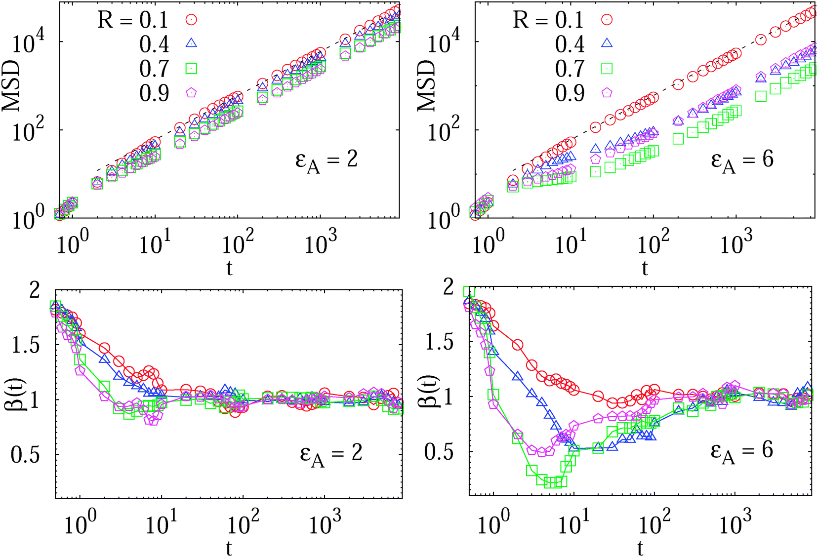

Fig. 3 MSD 〈r²(t)〉 of the tracer particles and the corresponding scaling exponent β(t), plotted for two trace–crowder attraction strengths, ε_A = 2 and 6, in units of . The result (8) for the MSD of three dimensional Brownian motion is represented by the dashed line in the MSD plots. The number of trajectories used for the averaging is N = 10³, and each trajectory consists of 10⁷ steps corresponding to the length T = 10⁴ of the simulated time series r(t) in terms of the simulation step δt = 10⁻³. Other parameters are as indicated in the plots. The obstacle radius is given in terms of R_max = a/2. The data sets for varying crowder radius are shown by open symbols.

Fig. 4 Long-time diffusivity D(ϕ)/D₀ in the terminal Brownian regime as function of the obstacle size, plotted for varying tracer–obstacle attraction strengths. Other parameters are the same as in Fig. 3. The dotted line represents the prediction by eqn (10) for inert obstacles. The data sets for varying adsorption strength are shown as filled symbols.

Let us look at these behaviours in some more detail. The variation of the scaling exponent β(t) with the crowding fraction and tracer–crowder attraction strength is shown in Fig. 3. We observe that as both ε_A and ϕ increase, the transient subdiffusion regime progressively extends over a larger time window. Remarkably, this anomalous diffusion spans up to two decades of time for substantial tracer–obstacle attraction strengths, see the plot of β(t) for in Fig. 3. For relatively weak tracer–obstacle attraction, at , only marginally anomalous tracer diffusion was detected, with β ∼ 0.85–1. Overall, the subdiffusion regime extends over one to two decades of time, similar to the results for inert static randomly-positioned obstacles⁶¹ or for the motion of tracers in a random channel with sticky surfaces.⁷²

A physically similar renormalisation of the particle diffusivity was discovered in ref. 73 for glassy states in sticky-particle systems at relatively large volume fractions ϕ. The phase diagram of the hard sphere mixture with a short range inter-particle attraction as well as a self-diffusive MSD dependence were examined, for instance, by simulations in ref. 73. The implications of the square-well sphere-sphere interaction potential ε_A and volume fraction ϕ of crowders were rationalised in detail. A progressive slowing down of the particle self-diffusion in the attractive hard-sphere mixtures as functions of ϕ and ε_A observed in Fig. 4 and 5 of ref. 73 is similar to the properties of the tracer diffusion on the lattice of moderately-sticky crowders examined here.

For non-attracting obstacles corresponding to ε_A = 0 the ratio D(ϕ)/D₀ of the diffusing coefficient of the tracer particle versus its value in an un-obstructed environment as function of the obstacle volume occupancy ϕ in a simple mean field approach is predicted to scale as

based on a volume exclusion argument in Section 8.3 of ref. 49. Here x = 2R/a is the relative obstacle size with respect to the lattice spacing. The reader is also referred to ref. 74 for the next-order corrections in the dependence of D(ϕ) on the volume fraction of crowders. Indeed, in absence of an attraction between the tracer and the obstacle surfaces, the behaviour of D(ϕ)/D₀ as function of R shown in Fig. 4 is in qualitative agreement with the prediction (10).

For moderate attraction, , the decrease of D(ϕ)/D₀ with R becomes less pronounced at R ≳ 0.6. For even stronger tracer–obstacle interaction, , remarkably the long-time diffusivity D(ϕ) becomes non-monotonic with the crowder size R, as shown in Fig. 4. Physically, at higher ϕ the available space for tracer diffusion becomes effectively reduced from the three dimensional volume to a lower dimensional space. This creates pathways or channels between the “cages” created by the obstacle and can effectively speed up the exploration of space by the tracer particle at higher ϕ fractions. Note that this effect would be modified when the surface diffusivity were considerably smaller than the volume diffusivity. However, as shown in the discussion of the trapping times below, another contribution to this speed up-effect could be that for larger crowder radius R the tracer is in a limbo between vicinal attractive surfaces and thus manoeuvres between obstacles without binding to them.

We note that in ref. 65 the diffusion coefficient of a tracer on an array of cylindrical obstacles on a static two dimensional square lattice was analysed in terms of the generalised Fick–Jacobs equation and by Brownian dynamics simulations. For the relative diffusivity as function of the crowding fraction ϕ the analogous behaviour D(ϕ)/D₀ = 1 − ϕ = 1 − π(R/R_max)²/4 was found, where π/4 is the maximal surface coverage in this situation.⁶⁵

B. Statistics of tracer trapping times

The non-monotonic dependence of the long-time tracer particle diffusivity on the crowding fraction is also manifested in the non-monotonic variation of the times that the tracer spends in the obstacle-adsorbed state. In Fig. 5 we present the statistics of individual adsorption times to the crowding particles along a long trajectory containing many binding–unbinding events. In the main graph of Fig. 5 we observe the distribution of tracer–obstacle adsorption times features a peak at short t_ads, while the tails of the histograms indicates the expected exponential decay. The corresponding mean adsorption time 〈t_ads〉 is the average over all the binding events encountered in our simulations for a particular set of the model parameters. As we can see, for larger crowders these exponential tails become progressively longer with increasing obstacle size up to some R < 0.6 × a/2, that is, the duration of binding events can become significantly longer. In the inset of Fig. 5 we use a logarithmic abscissa to pronounce the initial peak of the histograms. From this plot it becomes clear that several extremely long binding events can shift the mean 〈t_ads〉 of the binding time significantly, compare the relative positioning of the maximum of the histograms and the mean values indicated by the coloured dots.

Fig. 5 Histograms P(t_ads,i) of individual binding times t_ads,i spent in the obstacle-adsorbed state by the tracer particles, plotted for the parameters of Fig. 3 with attraction strength . The mean values 〈t_ads〉 for each crowder radius are indicated as the dots on the horizontal axis of the inset with the corresponding colour, indicating a non-monotonic behaviour with R. The main graph is shown in log-linear scale to show the exponential tails of the distributions, whereas the inset features a linear-log scale. The total length of the simulated trajectories is 10⁷ steps. The obstacle radius R is given in the legend in terms of R_max = a/2.

Thus, a small number of extremely long binding events govern the corresponding mean adsorption time 〈t_ads〉. Here, we mention the related study of ref. 75 in which the modes of surface versus bulk diffusion of a tracer in spherical domains were investigated. Also note that a different tracer diffusivity in the obstacle-bound mode as compared to the bulk diffusion can give rise to new interesting effects. In particular, an optimisation of the overall passage times of a tracer in the target-search problems on a lattice of trapping sites (obstacles) with a likely slower diffusivity should be analysed in the future.

Let us now turn to the total time of adsorption t_A experience by the tracer particle during a trajectory of duration T generated. We thus sum up all the adsorption times experienced by the tracer,

Adding to this quantity the excursion times in the bulk between the obstacles,we have T = t_A + t_B (the subscripts A and B denote the quantities in the adsorbed and bulk state, respectively). As expected, the total adsorption time t_A obtained from the simulations is an increasing function of the obstacle size R, compare Fig. 6. The initial increase of t_A with the crowder size R can be understood in terms of the concept of a “phantom sphere”. Namely, the surface of a crowding sphere available for surface diffusion by the crowding particles is S(R) = 4πR². If the remaining volume a³ − 4πR³/3 in a cubic unit cell framed by eight crowding spheres were converted into a (“phantom”) sphere, the surface of that sphere would amount toFollowing this crude argument to simply divide up the time spent on the surface of the crowders and on the phantom sphere surface (corresponding to the free volume of a unit cell in the obstacle lattice), the ratio of the adsorption time to the total time T of a sufficiently long trajectory can then be approximated aswhere we again used the dimensionless variable x = R/R_max = 2R/a. The maximal volume of the phantom sphere is given by the volume a³ of the unit cell, corresponding to an effective radius of the phantom sphere of R_max,ph = (a/2)(6/π)^1/3. The minimal effective radius of the phantom sphere corresponds to obstacles, which just touch each other on the square lattice, namely R_min,ph = (a/2)(6/π − 1)^1/3.

Fig. 6 Left: total diffusion time t_A in the adsorbed state of the tracer to the obstacle surface versus the obstacle size R, plotted in the log–log scale for varying binding strengths. Data obtained from averages of the histograms as those presented in Fig. 5. The dotted asymptote represents eqn (14). Right: plot of t_Aversus ε_A for varying obstacle radius. The dotted line indicates the exponential activation of t_A mentioned in the text. At higher ε_A a saturation of t_A is observed.

The ratio t_A/T given by eqn (14) is quadratic in the obstacle size R for small volume occupancy by obstacles. This result is in agreement with our simulations results for moderate tracer–obstacle binding, as shown in Fig. 6. In fact, for the attraction strength the agreement with result (14) is quite good given the simplicity of our model. In the shown double-logarithmic scale of Fig. 6 over the range R/R_max = 0.1–0.9 the law (14) in fact only weakly deviates from the quadratic scaling t_A/(t_A + t_B) ∼ (π/6)^2/3x². Naturally, the data for increasing binding affinity progressively deviate from the formula (14), for the strongest binding strength shown the particles move almost exclusively on the obstacle surface, independently of the obstacle size.

We observe that for small obstacle sizes and weak tracer–obstacle attraction strengths the total adsorption time t_A at fixed R grows exponentially with ε_A, , corresponding to the Boltzmann activation in an equilibrium system. As demonstrated in Fig. 6 on the right, for strong tracer–crowder attraction a saturation in t_A(ε_A) is reached, such that the activation curve for the ratio t_A/(t_A + t_B) is analogous to the expression for a simple two level system, . For larger crowders, when the tracers are confined predominantly to the obstacle surface, the saturation effect at larger attraction strengths is more pronounced, see Fig. 6.

In agreement with the results of Fig. 3 for the MSD, at moderate tracer–obstacle binding the adsorption time progressively increases for more voluminous obstacles on the lattice. In contrast, at strong tracer–crowder adsorption the adsorption time initially increases with the obstacle size

R = a[3ϕ/(4π)]^1/3 (15)

but above a critical volume fraction ϕ the value of t_Adecreases, as seen in Fig. 6 for the values and , as well as for the mean values shown in Fig. 5. This decrease of the mean adsorption time and thus a stronger contribution of bulk excursions is consistent with the non-monotonic dependence of D(ϕ)/D₀ at large tracer–obstacle binding strengths ε_A and with the enhanced diffusivity for larger strongly adhesive obstacles, see the curve for in Fig. 4. We ascribe this small yet somewhat counterintuitive effect to a competition of binding to neighbouring surfaces due to which the tracer particle is in a limbo in the bulk, possibly in conjunction with the reduced effective dimensionality of the environment mentioned above.

C. Time averaged MSD and non-Gaussianity parameter

To obtain more insight into the characteristics of the diffusive motion of the tracer particle in the crowded environment, we compute the time averaged MSD^15–19from the trajectory r(t) of the tracer of range t = 0,…,T. In eqn (16)Δ is the so-called lag time, which defines the size of a window slid along the trajectory r(t). The length of the trajectory T is also referred to as measurement time. In addition to the individual time traces we also consider the averageover N individual trajectories. When measured time series are not long enough, this quantity provides smoother curves if sufficiently many trajectories N are available.

In Fig. 7 we show the time averaged MSD (16) along with the MSD 〈r²(t)〉 of N = 100 individual trajectories. Let us first focus on the case of a moderate tracer–obstacle attraction strength, . We observe that the individual time traces initially grow ballistically and then cross over to normal diffusion, as indicated by the slopes in Fig. 7. The results for individual time traces show only minute amplitude variations at different lag times, quantitatively similar to the spread of time traces of regular Brownian particles. Of course, when Δ approaches the measurement time T, the statistics of the time average defining worsen and some amplitude scatter occurs.

The average (17) almost perfectly coincides with the ensemble average MSD 〈r²(t)〉, compare the blue and green curves in Fig. 7. The latter observation corroborates the ergodic nature of the tracer motion, that is, the equivalence of ensemble and long time average of physical observables, here .^15–17 The linear long time scaling of the MSD defines the effective diffusion coefficient D(ϕ) we shown in Fig. 4. Note that prolonged adsorption periods of the tracer on obstacle spheres correspond to effective trapping and delays the growth of either 〈x²(Δ)〉 or . For more information on the violation of the equivalence between time and ensemble averaged physical observables in anomalous-diffusive stochastic processes we refer to the recent review in ref. 17.

Fig. 7 MSD 〈r²(t)〉 (green curves) and time averaged MSD defined in eqn (16) (red curves), as well as the ensemble average (blue curves) over the simulated trajectories. Parameters are as indicated in the panels, the number of traces used for averaging is N = 100, and the length of the trajectories is T = 10⁴ corresponding to 10⁷ simulation steps.

As shown for the binding time statistics above, the trapping times are exponentially distributed and thus the long time motion converges to regular Brownian motion with a reduced, effective diffusivity D(ϕ). This scenario is therefore fundamentally different from subdiffusive CTRWs,^14,37 in which the characteristic trapping time diverges. Our Brownian motion-based physical rationale is consistent with experimental observations of protein diffusion in dense dextran solutions and with Monte-Carlo simulations of tracer diffusion on lattices of immobile inert obstacles as reported in ref. 56. In addition, we checked that the average time averaged MSD features no dependence on the trace length T: the values of almost perfectly overlap for different trace-lengths T, as demonstrated in Fig. 8 indicating the Brownian nature of the diffusion process.

Fig. 8 Independence of the time averaged MSD on the length T of the trajectory r(t). Parameters are the same as in Fig. 7.

A different situation is encountered when we consider strong tracer–obstacle attraction, in Fig. 7. We immediately observe that up to t = Δ ≈ 10² the time averaged MSD significantly differs from the corresponding ensemble average 〈r²(t)〉. That is, on these time scales the systems exhibits the disparity . For times exceeding t = Δ ≈ 10² the agreement between both quantities becomes excellent, the system is asymptotically ergodic. Individual curves for single time traces show a somewhat increased spread around their mean , however, this is still within the range expected for (asymptotically) ergodic processes,⁷⁶ and is significantly different from weakly non-ergodic processes such as subdiffusive CTRWs^{15–17,19,77} or heterogeneous diffusion processes.^17,42 For diffusion processes of the subdiffusive CTRW type the spread of individual time averaged MSD traces is expected to be finite even for vanishing lag times.^16,17 This kind of behaviour is definitely not observed in our simulations. Here a very narrow spread of in the whole range of tracer–obstacle affinities and obstacle sizes is observed, see, e.g., Fig. 7. The transient non-ergodic features observed here imply that the relaxation time towards ergodic behaviour is increased for longer trapping times when the tracer–obstacle attraction is more pronounced. The fact that the disparity is most pronounced around the turnover from initial ballistic to terminal Brownian motion is consistent with observations of confined stochastic processes driven by correlated Gaussian noise.^17,79

We now address a quantity that is based on the fourth order moment of the time trace . This non-Gaussianity parameter G(Δ) was shown to be a sensitive experimental indicator of the type of effective stochastic process driving the tracer particle in crowded complex fluids.⁵⁷ The non-Gaussianity parameter in three dimensions is defined by¹⁸

For diffusion processes with a stationary Gaussian distribution of increments such as Brownian motion and fractional Brownian motion we have G = 0, while the parameter G becomes non-zero for processes with non-stationary increments and/or non-Gaussian distributions such as subdiffusive CTRWs or heterogeneous diffusion processes.^44,57

We observe that for the simulated diffusion process in the presence of attractive obstacles the non-Gaussianity parameter shown in Fig. 9 is close to zero for almost the entire length of the traces, apart from the initial regime of the motion including inertial effects. These short time deviations from G ≈ 0 are particularly pronounced for relatively large obstacles with strong tracer–obstacle attraction, as shown for the different parameters analysed in Fig. 9. The fact that G ≈ 0 together with the equivalence of the ensemble and time averaged MSDs at sufficiently long times are, of course, a mirror for the Brownian nature of the observed motion. The smaller non-zero values of G detected in the long-time limit in Fig. 9 are due to small discrepancies between the ensemble and time averaged MSDs.

Fig. 9 Non-Gaussianity parameter (18) computed for the tracer diffusion on a lattice of sticky obstacles, the parameters are indicated. As a reference for almost perfect Gaussian behaviour G = 0, we present the non-Gaussianity parameter for vanishingly small, inert obstacles. The length of individual simulated trajectories is T = 10⁴.

At short to moderate times the non-Gaussianity parameter substantially deviates from the zero value characteristic of Brownian motion for strongly adhesive and relatively large crowders, see, e.g., the blue curve in Fig. 9. The deviations of G(Δ) occur at time scales of t ∼ 1–30 when the tracer diffusion is inherently non-ergodic, as we see from the right panel of Fig. 7 plotted for the same parameters ( and R/R_max = 0.6). At very short times, t ≪ 1, on which the MSD and time averaged MSD coincide, the non-Gaussianity parameter respectively assumes very small values. Otherwise, the deviations from G = 0 we observe are within the range typically measured in experiments⁵⁷ for asymptotically ergodic stationary-increment processes.

IV. Conclusions

We studied the passive motion of a tracer particle in an ordered, stationary array of attractive spherical crowders. Based on a truncated attractive Lennard Jones interaction between tracer and crowding obstacles, we simulate long individual trajectories of the tracer based on the Langevin equation. The resulting motion features a transition from initial ballistic flights corresponding to the inertial particle motion to a long time Brownian diffusion behaviour. The magnitude of the effective diffusion coefficient of this terminal Brownian motion is reduced for increasing obstacle volume filling fraction and tracer–obstacle attraction. However, a distinct non-monotonicity in this behaviour for large obstacle radii and high attraction strength is observed, likely due to competing attraction from multiple obstacles for which the tracer particle is in a limbo in the bulk. The same effect also leads to a decrease of the time t_A(ϕ) spent adsorbed to the obstacle surfaces during a long trajectory. The long time Brownian dynamics was consistently shown to be associated with approximately vanishing non-Gaussianity parameter. These dynamic features point out the crucial role of varying tracer–obstacle binding strengths in the analysis of crowded systems, as performed here. To put these qualitative statements on a more physical foundation, additional simulations will be necessary. In particular, we will study the time averaged van Hove cross-correlation functions⁷⁸ for the tracer motion.

At intermediate times the tracer particle motion is anomalous, with a distinctly time-dependent scaling exponent β(t). In this regime the trapping to the obstacles becomes the dominant mechanism. According to our results the time and ensemble averaged MSDs are equivalent for moderate tracer–obstacle attraction strength, however, a transient non-ergodic disparity between the two observables is observed over a range of some 2.5 orders of magnitude for stronger tracer–crowder binding. This transient form of weakly non-ergodic behaviour was previously observed for correlated Gaussian processes under confinement^34,79 of the otherwise ergodic process.³⁹ This behaviour should be kept in mind when precise diffusive properties are to be analysed from measured or simulated time traces of our system.

Extensions of the current model should consider a range of surface diffusivities of tracer particles bound to obstacles. Moreover, the arrangement of crowders should release the static, ordered arrangement on a lattice. Thus, off-lattice simulations could include the motion of crowders around their equilibrium positions, similarly to the analysis in ref. 53. Differences in the sizes of individual crowders and a certain randomness in the tracer–obstacle affinity would be additional relevant generalisations of the current system. Mobile obstacles were shown to profoundly reduce the time range of the transient subdiffusive motion compared to immobile crowders.⁵³ However, the generality of these findings needs to be explored in a broader parameter range. Currently, it remains elusive to arrive at realistic models capturing the richness of real MMC effects in living biological cells with their wide variety of crowder shapes, surface properties, persistence length and degree of branching as well as a poly-disperse size distribution, in addition to cellular structural elements, as well as charge effects.⁵ Finally, active processes such as energy-consuming transport in living cells^35,80,81 needs to be added to achieve a closed picture of all facets of cellular dynamics.

Our study complements several other recent analyses of tracer motion in crowded environments. Thus, tracer diffusion in a system of relaxed and stretched polymer chains in the presence of tracer–polymer attraction was studied by Langevin dynamics simulations with the Espresso package.⁸² We observe that such obstructed diffusion with sticky obstacles resembles our current results. For instance, the evolution of the time-dependent MSD scaling exponent β (see Fig. 4 in ref. 82) shows a transition from the initial ballistic regime to a subdiffusive regime at intermediate times, and further to Brownian motion in the long-time limit. The anomalous diffusion regime was shown to span a larger time window for the relaxed as compared to the stretched self-avoiding chains.⁸² Higher polymer densities and stronger tracer–polymer interactions yield wider regions of tracer subdiffusion.⁸² A continuation of this study for tracer diffusion in a cylindrical pore with surface-grafted polymer brushes of varying density showed that the subdiffusive regime is more pronounced for weak-to-moderate tracer–polymer interaction.⁶⁶

We also mention an experimental study of impeded colloidal diffusion in transient polymer networks with varying colloid–polymer binding interactions.⁸³ For the diffusion of an inert tracer in a responsive elastic network system, when the tracer size is of the same order as the unit cell of this gel, transient subdiffusion was reported and shown to involve characteristic collective dynamics of tracer and gel.⁷⁸ The transient subdiffusion in this study is in contrast to the experimentally observed long-tailed distribution of trapping times of sub-micron tracers in semi-flexible, inherently dynamic networks of cross-linked actin⁸⁴ and thus further underlines the non-universal character of the dynamics in crowded systems. We finally mention that diffusion in two-dimensional, oriented fibrous networks in the presence of repulsive and attractive particle–obstacle interactions was in fact studied experimentally in connection with hydrogel-like structures of the extracellular matrix.⁸⁵

Is crowding in cells merely an effect of cramming a rich multitude of different bio-molecules into a minimal volume, or does it have an evolutionary purpose in giving rise to dynamic phenomenon such as (transient) subdiffusion?^21,86 The combination of advanced single particle technology and other experimental methods along with improved in silico studies will lead to significant advances in the understanding of these still elusive questions.

Acknowledgements

The authors acknowledge funding from the Academy of Finland (FiDiPro scheme to RM), the German Research Foundation (DFG Grant CH 707/5-1 to AGC), and the German Ministry of Education and Research (BMBF Grant to SG).

References

1. S. B. Zimmerman and S. O. Trach, J. Mol. Biol., 1991, 222, 599.
2. S. B. Zimmerman and A. P. Minton, Annu. Rev. Biophys. Biomol. Struct., 1993, 22, 27.
3. D. Hall and A. P. Minton, Biochim. Biophys. Acta, 2003, 1649, 127.
4. H. X. Zhou, J. Mol. Recognit., 2004, 17, 368.
5. A. R. McGuffee and A. H. Elcock, PLoS Comput. Biol., 2010, 6, e1000694.
6. R. J. Ellis, Curr. Opin. Struct. Biol., 2001, 11, 114.
7. A. P. Minton, J. Biol. Chem., 2001, 276, 10577.
8. A. P. Minton, Biopolymers, 1981, 20, 2093.
9. H. X. Zhou, G. Rivas and A. P. Minton, Annu. Rev. Biophys., 2008, 37, 375.
10. C. Echeverria and R. Kapral, Phys. Chem. Chem. Phys., 2012, 14, 6755.
11. E. Spruijt, E. Sokolova and W. T. S. Huck, Nat. Nanotechnol., 2014, 9, 406.
12. J. Shin, A. G. Cherstvy and R. Metzler, New J. Phys., 2014, 16, 053047.
13. J. P. Bouchaud and A. Georges, Phys. Rep., 1990, 195, 127.
14. R. Metzler and J. Klafter, Phys. Rep., 2000, 339, 1.
15. E. Barkai, Y. Garini and R. Metzler, Phys. Today, 2012, 65(8), 29.
16. S. Burov, J.-H. Jeon, R. Metzler and E. Barkai, Phys. Chem. Chem. Phys., 2011, 13, 1800.
17. R. Metzler, J.-H. Jeon, A. G. Cherstvy and E. Barkai, Phys. Chem. Chem. Phys., 2014, 16, 24128.
18. F. Höfling and T. Franosch, Rep. Prog. Phys., 2013, 76, 046602.
19. I. M. Sokolov, Soft Matter, 2012, 8, 9043.
20. M. Wachsmuth, W. Waldeck and J. Langowski, J. Mol. Biol., 2000, 298, 677.
21. I. Golding and E. C. Cox, Phys. Rev. Lett., 2006, 96, 098102; S. C. Weber, A. J. Spakowitz and J. A. Theriot, Phys. Rev. Lett., 2010, 104, 238102.
22. I. Bronstein, et al. , Phys. Rev. Lett., 2009, 103, 018102; K. Burnecki, E. Kepten, J. Janczura, I. Bronshtein, Y. Garini and A. Weron, Biophys. J., 2012, 103, 1839.
23. M. Platani, I. Goldberg, A. I. Lamond and J. R. Swedlow, Nat. Cell Biol., 2002, 4, 502.
24. J.-H. Jeon, et al. , Phys. Rev. Lett., 2011, 106, 048103; M. A. Tabei, S. Burov, H. Y. Kim, A. Kuznetsov, T. Huynh, J. Jureller, L. H. Philipson, A. R. Dinner and N. F. Scherer, Proc. Natl. Acad. Sci. U. S. A., 2013, 110, 4911.
25. G. Seisenberger, et al. , Science, 2001, 294, 1929.
26. C. Brauchle, et al. , ChemPhysChem, 2002, 3, 299.
27. M. R. Horton, F. Höfling, J. O. Rädler and T. Franosch, Soft Matter, 2010, 6, 2648.
28. J. Ehrig, E. P. Petrov and P. Schwille, Biophys. J., 2011, 100, 80.
29. J.-H. Jeon, H. M. S. Monne, M. Javanainen and R. Metzler, Phys. Rev. Lett., 2012, 109, 188103; G. R. Kneller, K. Baczynski and M. Pasienkewicz-Gierula, J. Chem. Phys., 2011, 135, 141105; M. Javanainen, H. Hammaren, L. Monticelli, J.-H. Jeon, R. Metzler and I. Vattulainen, Faraday Discuss., 2013, 161, 397.
30. E. Yamamoto, T. Akimoto, M. Yasui and K. Yasuoka, Sci. Rep., 2014, 4, 4720.
31. A. S. Kozlov, D. Andor-Ardo and A. J. Hudspeth, Proc. Natl. Acad. Sci. U. S. A., 2012, 109, 2896.
32. D. S. Banks and C. Fradin, Biophys. J., 2005, 89, 2960.
33. G. Guigas, C. Kalla and M. Weiss, Biophys. J., 2007, 93, 316; W. Pan, L. Filobelo, N. D. Q. Pham, O. Galkin, V. V. Uzunova and P. G. Vekilov, Phys. Rev. Lett., 2009, 102, 058101.
34. J.-H. Jeon, N. Leijnse, L. B. Oddershede and R. Metzler, New J. Phys., 2013, 15, 045011.
35. D. Robert, Th.-H. Nguyen, F. Gallet and C. Wilhelm, PLoS One, 2010, 4, e10046; I. Goychuk, V. O. Kharchenko and R. Metzler, PLoS One, 2014, 9, e91700; I. Goychuk, V. O. Kharchenko and R. Metzler, Phys. Chem. Chem. Phys., 2014, 16, 16524.
36. O. Chepizhko and F. Peruani, Phys. Rev. Lett., 2013, 111, 160604.
37. E. W. Montroll and G. H. Weiss, J. Math. Phys., 1969, 10, 753; H. Scher and E. W. Montroll, Phys. Rev. B: Solid State, 1975, 12, 2455.
38. B. B. Mandelbrot and J. W. van Ness, SIAM Rev., 1968, 10, 422.
39. W. Deng and E. Barkai, Phys. Rev. E: Stat., Nonlinear, Soft Matter Phys., 2009, 79, 011112.
40. E. Lutz, Phys. Rev. E: Stat., Nonlinear, Soft Matter Phys., 2001, 64, 051106.
41. I. Goychuk, Phys. Rev. E: Stat., Nonlinear, Soft Matter Phys., 2009, 80, 046125; I. Goychuk, Adv. Chem. Phys., 2012, 150, 187.
42. A. G. Cherstvy, A. V. Chechkin and R. Metzler, New J. Phys., 2013, 15, 083039; A. G. Cherstvy and R. Metzler, Phys. Chem. Chem. Phys., 2013, 15, 20220.
43. P. Massignan, C. Manzo, J. A. Torreno-Pina, M. F. Garca-Parako, M. Lewenstein and G. L. Lapeyre, Jr., Phys. Rev. Lett., 2014, 112, 150603.
44. A. G. Cherstvy and R. Metzler, Phys. Rev. E: Stat., Nonlinear, Soft Matter Phys., 2014, 90, 012134.
45. A. Fulinski, J. Chem. Phys., 2013, 138, 021101; A. Fulinski, Phys. Rev. E: Stat., Nonlinear, Soft Matter Phys., 2011, 83, 061140.
46. S. C. Lim and S. V. Muniandy, Phys. Rev. E: Stat., Nonlinear, Soft Matter Phys., 2002, 66, 021114.
47. F. Thiel and I. M. Sokolov, Phys. Rev. E: Stat., Nonlinear, Soft Matter Phys., 2014, 89, 012115; J.-H. Jeon, A. V. Chechkin and R. Metzler, Phys. Chem. Chem. Phys., 2014, 16, 15811.
48. J. P. Bouchaud, A. Comtet, A. Georges and P. le Doussal, Ann. Phys., 1990, 201, 285.
49. J. W. Haus and K. W. Kehr, Phys. Rep., 1987, 150, 263.
50. E. Bertin and J.-P. Bouchaud, Phys. Rev. E: Stat., Nonlinear, Soft Matter Phys., 2003, 67, 026128; C. Monthus and J.-P. Bouchaud, J. Phys. A: Math. Gen., 1996, 29, 3847; S. Burov and E. Barkai, Phys. Rev. Lett., 2007, 98, 250601.
51. A. Sikorski and P. Polanowski, Soft Matter, 2014, 10, 3597.
52. H. Berry and H. Chaté, arXiv:1103.2206.
53. H. Berry and H. Chaté, Phys. Rev. E: Stat., Nonlinear, Soft Matter Phys., 2014, 89, 022708; H. Soula, B. Caré, G. Beslon and H. Berry, Biophys. J., 2013, 105, 2064.
54. Moreover, in ref. 52 the distribution of particle trapping times in dynamical cages formed between the crowders was shown to be inconsistent with the CTRW model, as observed in simulations for mobile crowders, crowders confined in a potential, and static obstacles. Namely, the power-law distribution of trapping times ψ(τ) ∼ τ^−γ was shown to range between γ = 3.5–4, in contrast to the range γ = 1–2 expected for subdiffusive CTRW processes with diverging characteristic waiting time^15–17.
55. T. K. Piskorz and A. Ochab-Marcinek, J. Phys. Chem. B, 2014, 118, 4906.
56. J. Szymanski and M. Weiss, Phys. Rev. Lett., 2009, 103, 038102.
57. D. Ernst, J. Koehler and M. Weiss, Phys. Chem. Chem. Phys., 2014, 16, 7686.
58. M. J. Saxton, Biophys. J., 1987, 52, 990.
59. M. J. Saxton, Biophys. J., 1996, 70, 1250.
60. M. J. Saxton, Biophys. J., 2010, 99, 1490.
61. P. A. Netz and T. Dorfmuller, J. Chem. Phys., 1997, 107, 9221.
62. Y. Meroz, I. M. Sokolov and J. Klafter, Phys. Rev. E: Stat., Nonlinear, Soft Matter Phys., 2010, 81, 010101(R).
63. F. Höfling, T. Franosch and E. Frey, Phys. Rev. Lett., 2006, 96, 165901.
64. M. Spanner, et al. , J. Phys.: Condens. Matter, 2011, 23, 234120.
65. L. Dagdug, M. V. Vazquez, A. M. Berezhkovskii, V. Yu. Zitserman and S. M. Bezrukov, J. Chem. Phys., 2012, 136, 204106.
66. R. Chakrabarti, S. Kesselheim, P. Kosovan and C. Holm, Phys. Rev. E: Stat., Nonlinear, Soft Matter Phys., 2013, 87, 062709.
67. N. A. Mahynski, A. Z. Panagiotopoulos, D. Meng and S. K. Kumar, Nat. Commun., 2014, 5, 4472.
68. M. A. Lomholt, I. M. Zaid and R. Metzler, Phys. Rev. Lett., 2007, 98, 200603; A. V. Chechkin, I. M. Zaid, M. A. Lomholt, I. M. Sokolov and R. Metzler, Phys. Rev. E: Stat., Nonlinear, Soft Matter Phys., 2012, 86, 041101.
69. R. Huang, I. Chavez, K. M. Taute, B. Lukic, S. Jeney, M. G. Raizen and E.-L. Florin, Nat. Phys., 2011, 7, 576.
70. D. S. Grebenkov, M. Vahabi, E. Bertseva, L. Forro and S. Jeney, Phys. Rev. E: Stat., Nonlinear, Soft Matter Phys., 2013, 88, 040701(R).
71. W. T. Coffey and Y. P. Kalmykov, The Langevin equation, World Scientific, Singapore, 2012.
72. M. Bauer, A. Godec and R. Metzler, Phys. Chem. Chem. Phys., 2014, 16, 6118.
73. E. Zaccarelli and W. C. K. Poon, Proc. Natl. Acad. Sci. U. S. A., 2009, 106, 15203.
74. J. Balbo, P. Mereghetti, D. P. Herten and R. C. Wade, Biophys. J., 2013, 104, 1576.
75. J.-F. Rupprecht, O. Benichou, D. S. Grebenkov and R. Voituriez, J. Stat. Phys., 2012, 147, 891.
76. J.-H. Jeon and R. Metzler, J. Phys. A: Math. Gen., 2010, 43, 252001.
77. A. Lubelski, I. M. Sokolov and J. Klafter, Phys. Rev. Lett., 2008, 100, 250602; Y. He, S. Burov, R. Metzler and E. Barkai, Phys. Rev. Lett., 2008, 101, 058101.
78. A. Godec, M. Bauer and R. Metzler, New J. Phys., 2014, 16, 092002.
79. J.-H. Jeon and R. Metzler, Phys. Rev. E: Stat., Nonlinear, Soft Matter Phys., 2012, 85, 021147.
80. A. Caspi, R. Granek and M. Elbaum, Phys. Rev. Lett., 2000, 85, 5655.
81. S. Leitmann and T. Franosch, Phys. Rev. Lett., 2013, 111, 190603.
82. F. Tabatabaei, O. Lenz and C. Holm, Colloid Polym. Sci., 2011, 289, 523.
83. J. Sprakel, J. van der Gucht, M. A. Cohen-Stuart and A. M. Besseling, Phys. Rev. E: Stat., Nonlinear, Soft Matter Phys., 2008, 77, 061502.
84. I. Y. Wong, et al. , Phys. Rev. Lett., 2004, 92, 178101.
85. O. Lieleg, R. M. Baumgartel and A. R. Bausch, Biophys. J., 2009, 97, 1569.
86. G. Guigas and M. Weiss, Biophys. J., 2008, 94, 90; M. Hellmann, D. W. Heermann and M. Weiss, Europhys. Lett., 2011, 94, 18002; L. E. Sereshki, M. A. Lomholt and R. Metzler, Europhys. Lett., 2012, 97, 20008.
87. To map the exchange between the bulk and a reactive surface (here defined via the attractive part of the potential (3)) onto a random walk picture, compare ref. 68.

---