Tunable picosecond spin dynamics in two dimensional ferromagnetic nanodot arrays with varying lattice symmetry

Abstract

The in-plane configurational anisotropy of the frequency and nature of spin-wave modes in two-dimensional artificial Ni₈₀Fe₂₀ nanodot lattices arranged in closely packed rectangular, honeycomb and octagonal lattices are demonstrated by time-resolved magneto-optical Kerr effect measurements. The rectangular, honeycomb and octagonal lattices showed dominant two-fold, six-fold and eight-fold variation of frequency superposed with a weak four-fold anisotropy for specific spin-wave modes with the variation of the azimuthal angle of the external bias magnetic field. Micromagnetic simulations reveal that the observed anisotropy is due to the angular variation of the magnetostatic field distribution and the ensuing spin-wave mode profiles, which varies between arrays. The observations are important for selecting building blocks for future magnetic data storage and magnonic crystals for on-chip microwave communication and processing.

---

Introduction

Magnonic crystals (MCs)^1–6 are artificial crystals with periodic modulation of magnetic properties where spin-waves (SWs) are the transmission waves. MCs form magnonic minibands consisting of allowed and forbidden SW frequencies and corresponding magnonic bandgaps. The SWs in MCs can be controlled by changing their various physical and geometrical parameters such as material,^7–9 shape,^10,11 size, lattice spacing,¹² lattice symmetry,^13,14 as well as strength and orientation of the external bias field.^10,15 This tunability of MCs makes them a potential candidate for on-chip microwave communication devices and components, including magnonic waveguides,¹⁶ filters,¹⁷ splitters, phase shifters,¹⁸ spin-wave emitters,¹⁹ as well as for magnonic logic devices.^20,21 In case of photonic crystals it is reported²² that the anisotropy of photonic bandgap is dependent on the symmetry of the photonic crystal lattices. As the symmetry increases the Brillouin zone becomes more circular, resulting in a complete band gap. The highest order symmetry observed in a periodic lattice is six-fold, however, higher levels of symmetry can be potentially achieved by using complex geometries of quasicrystals.²³ It is well known that the spin and orbital angular momentum is responsible for the magnetic properties of solid. The violation of spin orbit angular momentum with respect to the rotation of magnetization direction leads to the concept of basic magnetic anisotropy. The magnetization at the edges of a confined magnetic element deviates from the external field direction to minimize the magnetic energies. These regions are known as the demagnetized regions. Consequently, the average magnetization and the internal magnetic field changes with the rotation of the azimuthal angle of the external bias field. This is known as intrinsic configurational anisotropy.^24,25 The effective magnetic field inside an element within an array is modified due to the stray field from the neighbouring elements. The tailoring of this field by rotating the bias field angle with respect the symmetry axes of the array leads to the occurrence of extrinsic configurational anisotropy.¹⁵

It is already reported¹⁴ that lattice symmetry of two-dimensional nanodot arrays plays a significant role in their SW spectra. The single uniform collective mode in a square lattice splits into two modes in the rectangular lattice and into three modes in both the hexagonal and octagonal lattices. However, in the honeycomb lattice a broad band of modes is observed. This is due to a large variation of the stray field causing the inter-dot interaction. For such systems rotation of the azimuthal angle of the external bias field may lead to interesting extrinsic configurational anisotropy in the collective magnetization dynamics according to the lattice arrangements. Here, we investigate the above possible configurational anisotropy in circular nanodot arrays arranged in rectangular, honeycomb and octagonal lattices. We previously reported that the square and hexagonal lattices exhibit a four-fold²⁶ and a six-fold configurational anisotropy,^14,27 respectively. Here, we show that for the rectangular, honeycomb and octagonal lattices the most intense peak shows primarily two-fold, six-fold and eight-fold anisotropies superposed with a relatively weak four-fold anisotropy due to the shape of the boundary of the arrays.

Experimental details

10 × 10 μm² arrays of 20 nm thick Ni₈₀Fe₂₀ dots with negligible magneto crystalline anisotropy and with circular shapes arranged in rectangular, honeycomb and octagonal lattices are fabricated by a combination of electron beam lithography and electron beam evaporation. The diameter of individual dots is about 100 nm and the edge-to-edge separation between the dots is about 30 nm. The dot shape, size and the inter-dot separation are chosen to ensure negligible shape anisotropy, accommodation of two intrinsic modes^8,28 (edge and centre modes) inside the dots and a strongly collective magnetization dynamics of the array.

The ultrafast magnetization dynamics of the samples is measured by an all-optical time-resolved magneto-optical Kerr effect microscope based upon a two-color collinear pump–probe geometry.²⁹ The second harmonic (λ = 400 nm, pulse width ∼100 fs) of a mode-locked Ti-sapphire laser (Tsunami, Spectra Physics) is used to excite the magnetization dynamics in the sample whereas the time-delayed fundamental (λ = 800 nm, pulse width ∼80 fs) is used to probe the dynamics by measuring the Kerr rotation as a function of the time-delay between the pump and probe beams. The pump and probe beams are made collinear and are focused onto the centre of the whole array by using a microscope objective (N.A. = 0.65) to spot sizes of 1 μm and 800 nm, respectively to measure the local magnetization dynamics under the focused laser spot. An external magnetic field (H) is applied at a small angle (10°) to the sample plane. In the experimental set up, we effectively vary the azimuthal angle (φ) of H between 0° and 180° at intervals of 5°, 10° and 15° for octagonal, honeycomb and rectangular lattice, respectively. This is done by rotating the samples using a high precision rotary stage while keeping the microscope objective and H constant. The pump and the probe beams are made to incident on the same region of the array for each value of φ.

Results and discussions

Fig. 1(a) represents a typical time-resolved Kerr rotation data for octagonal lattice at a bias field H = 1.3 kOe at φ = 0°. The data in the left panel shows an ultrafast demagnetization within 500 fs with a bi-exponential decay with decay constants of 3 ps and 400 ps. The precessional dynamics appears as an oscillatory signal on the slowly decaying part of the time-resolved Kerr rotation data. The background subtracted Kerr rotation data is shown in the right panel. In Fig. 1(b) simulated hysteresis loops for arrays with three different lattice symmetries at φ = 0° are shown, which will be discussed later in this article. The fast Fourier transformations (FFTs) of the time resolved data reveal the SW spectra as shown in Fig. 1(c) for the rectangular, honeycomb and octagonal lattices at φ = 0°, 30° and 90°. The corresponding SEM images of the lattices are shown in the inset. The experimental geometry is shown on the SEM image of the rectangular lattice. A clear difference is observed in the SW spectra both with the variation of the lattice arrangement and φ. The solid curves correspond to theoretical fits to harmonic functions with anisotropies having different symmetries (Fig. 2(a) and (b)). The rectangular lattice shows two modes for all φ values (Fig. 1(c)), and the lower frequency mode (asterisk marked) shows a combination of two-fold (88%) and four-fold (12%) anisotropies (Fig. 2(a)) from the theoretical fit. For honeycomb lattice the situation is quite different. A broad band of modes for φ = 0° transforms to a single mode with a small splitting at φ = 30°. As φ increases further new modes start to appear and at φ = 45° two modes with a small splitting are observed while for 60° ≤ φ ≤ 90° again broad band of modes appear. This phenomenon is repeated with a period of 90°. The frequency of the asterisk marked mode first decreases as φ deviates from 0°. At φ = 30° the frequency attains a minimum value and it increases again as φ changes from 30° and a maxima is obtained φ = 60°. This phenomenon is repeated and at φ = 30°, 90° and 150° minima are observed whereas at φ = 0°, 60°, 120° and 180° maxima is observed as shown in Fig. 2(a). Theoretical fitting of the variation of this mode frequency with φ shows a combination of six-fold (83%) and four-fold (17%) anisotropies. For octagonal lattice, three modes (Fig. 1(c)) are observed at φ = 0° and the number of modes remained the same for all values of φ except for variation in their relative intensities. The asterisk marked mode corresponding to f = 8.84 GHz shows a combination of eight-fold (90%) and four-fold (10%) anisotropies as shown in Fig. 2(a). To understand the origin of these anisotropies, we have performed micromagnetic simulations at T = 0 K using the OOMMF software³⁰ on 1100 × 1100 × 20 nm³ volume consisting of circular dots arranged in different lattice symmetries. The sample geometries for the simulation are derived from the SEM image of the samples. The simulated array volumes are considered smaller than the experimental samples due to computational resources. However, they are larger than the excitation and probe volumes used in the experiment and are expected to capture the experimental observations well. The samples are discretized into rectangular prism-like cells with dimensions 2 × 2 × 20 nm³. Discretization of circular nanodots by rectangular prism like cells introduces some artificial edge roughness but this is negligible compared to the dimensions of the nanodots and does not affect the dynamics significantly. The lateral cell size is well below the exchange length of Py (5.3 nm). The parameters used for the simulation are γ = 18.5 MHz Oe⁻¹, exchange stiffness constant, A = 1.3 × 10⁻⁶ erg cm⁻¹, magnetocrystalline anisotropy constant K = 0 and saturation magnetization M_s = 860 emu cm⁻³. The static and the dynamic simulations are performed by methods described elsewhere.³¹ First, we simulated the hysteresis loop for arrays with three different lattice symmetries (Fig. 1(b)) at φ = 0°. The loops vary significantly between different arrays. The rectangular lattice shows a small corrective field (H_c = 14 Oe) and saturation field (H_S = 0.35 kOe), which increase significantly in honeycomb (H_c = 135 Oe, H_S = 0.9 kOe) and octagonal (H_c = 122 Oe, H_S = 1.05 kOe) lattices. The external bias field H (>H_S for all arrays) is applied according to the experimental configuration and a pulsed field of rise time of 50 ps and peak amplitude of 30 Oe is applied perpendicular to the sample plane. The optical excitation used in the experiment is simulated as a pulsed magnetic field, which is a valid approximation as within few picoseconds of the optical excitation the energy from the spin and electron systems are transferred to the lattice, which effectively launches a pulsed magnetic field within the system and triggers the SW dynamics as studied here.

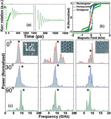Fig. 1 (a) Typical experimental time-resolved Kerr rotation data from the octagonal lattice at H = 1.3 kOe revealing ultrafast demagnetization, fast and slow relaxations, and precession of magnetization (left panel). Background subtracted time-resolved Kerr rotation data is shown in the right panel. (b) Simulated magnetic hysteresis loops for arrays with three different lattice symmetries at φ = 0°. (c) The SW spectra obtained by FFT of the time-resolved data from rectangular, honeycomb and octagonal lattices are shown for different values of φ at H = 1.3 kOe. The corresponding scanning electron micrographs with the schematic of the experimental geometry are shown in the insets.

Fig. 2 (a) Experimental and (b) simulated SW frequencies (symbols) as a function of the azimuthal angle φ of the in-plane bias magnetic field at H = 1.3 kOe. The solid curves show the theoretical fits.

The dynamic simulations were acquired for 1.5 ns at the time steps of 5 ps. The experimental results are qualitatively reproduced by the simulations. In Fig. 2(b), the simulated mode frequencies for different lattices are plotted as a function of φ. The simulations reproduced the major experimentally observed features. Theoretical fits to the simulated results reveal the presence of two-fold, six-fold and eight-fold anisotropy, superposed with a four-fold anisotropy for rectangular, honeycomb and octagonal lattice, respectively. The fits are reasonable for both experimental and simulated data, and the deviations are possibly due to the edge roughness and irregularities in the samples, which modify the anisotropy arising due to the symmetry of the stray magnetic field in this lattice. There are primarily three contributions to the configurational anisotropy – (1) the shape of the array boundary (2) the lattice symmetry and (3) the shape of the individual dot. The first contribution arises due to the strongly collective magnetization dynamics, the second contribution originates from inter-dot the magnetostatic stray fields and the ensuing change in the internal fields of the constituent nanodots while the third contribution is not applicable in our case as the dot shapes are circular.

Simulated angular variation of the mode profiles of the collective modes in arrays with different lattice symmetry

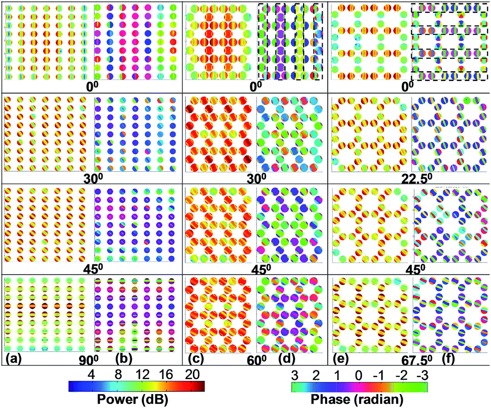
We have further simulated the angular variations of mode profile³² of the studied modes for samples with different lattice symmetry. The power maps of the modes for rectangular, honeycomb and octagonal lattices at different φ values are shown in Fig. 3. For the rectangular lattice (Fig. 3(a)), the anisotropic mode at φ = 0° corresponds to the edge mode of the individual nanodots distributed uniformly over the entire lattice barring the vertical edges. With the variation of φ the edge modes in the dots and their distribution in the array rotate following the bias field. Clearly the stronger interaction between the edge modes of the dots along the vertical direction (smaller lattice constant) gives the stronger two-fold anisotropy while the square boundary of the array gives the weaker four-fold anisotropy due to the collective dynamics of the array. The honeycomb lattice shows a number of modes at φ = 0° but the only anisotropic mode correspond to vertical stripe-like regions, where the half circles (full circle) are alternatively precessing in-phase and out-of-phase with each other (dotted boxes in Fig. 3(e)) forming a collective backward volume (BV) like mode of the array.¹⁴ As φ increases from 0° the collective BV like mode breaks down giving rise to a complicated mode profile. In addition, the distribution of the power of the mode at the central part of the array varies, first decreasing as φ increases from 0° to 30° and then increasing as φ increases further to 60°. For the octagonal lattice the anisotropic mode corresponds to the BV like modes of the nanodots collectively precessing in phase within the regions shown by the dotted boxes (Fig. 3(f)) at φ = 0°. As φ increases the collective modes of the arrays break down. In addition, the power map shows that the BV like mode of the constituent dots converts to edge mode of the dots at 22.5°, reappears at 45° and turns into edge modes again at 67.5° and is repeated in this fashion. Since the edge mode has lower frequency than the BV like mode the mode frequency varies with that period.

Fig. 3 The power ((a), (c) and (e)) and phase ((b), (d) and (f)) maps of the asterisk (*) marked modes for the rectangular ((a) and (b)), honeycomb ((c) and (d)) and octagonal ((e) and (f)) lattices for selected values of φ at H = 1.3 kOe. The color maps for power and phase distributions are shown at the bottom of the figure.

Angular variation of simulated magnetostatic field distributions for arrays with different lattice symmetry

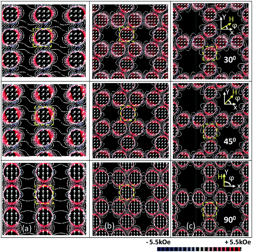
Although the SW mode profiles give some indication about the origin of the observed configurational anisotropy, we have further studied the variation of magnetostatic field distribution in the arrays with the bias field angle φ. The magnetostatic field consists of dipolar and higher order multipolar fields as well as localized fields in some cases. Fig. 4 shows the contour plots of the above field for different lattices at φ = 30°, 45° and 90°, while the arrows represent the magnetization inside the dots and the schematic shows the direction of the applied bias field. The stray fields as well as the internal fields change considerably with the variation of φ leading towards the variation in the observed mode structures as well as the mode frequencies. We have further estimated the variation of the average magnetic field acting on a single dot from the array shown by the dotted boxes in Fig. 4 with φ and found a similar anisotropy in the magnetic field itself as shown in Fig. 5. Theoretical fitting with the data in Fig. 5 revealed two-fold, six-fold and eight-fold anisotropy superposed with a weak four-fold anisotropy for the rectangular, honeycomb and octagonal lattice, respectively. This variation is a result of the magnetic environment of the dots in different lattices and its ensuing variation with the angle of the bias field, and is manifested as the configurational anisotropy in the samples.

Fig. 4 Contour maps of simulated magnetostatic field distributions (x-component) are shown for (a) rectangular, (b) honeycomb and (c) octagonal lattice for selected values of φ at H = 1.3 kOe. The schematics of the applied bias field directions are also shown for all values of φ. The color map for the magnetostatic field is shown at the bottom of the figure.

Fig. 5 Variation of the simulated average magnetostatic field as a function of φ at H = 1.3 kOe from samples with different lattice symmetry. The symbols show simulated data, while the solid curves show the theoretical fits.

Conclusions

In conclusion, we have investigated the configurational anisotropy in the precessional magnetization dynamics in two dimensional ferromagnetic nanodot lattices with different lattice symmetries. The azimuthal angle of the bias magnetic field is varied between 0° and 180° and the SW spectrum showed a drastic variation in number of peaks and peak positions with the angle. The dominant precessional mode showed two-fold, six-fold and eight-fold anisotropy superposed with a weak four-fold anisotropy for rectangular, honeycomb and octagonal lattice, respectively. The four-fold anisotropy originates due to the square boundaries of the arrays as a result of the collective magnetization dynamics, whereas two-fold, six-fold and eight-fold anisotropies arise due to the variation of the magnetostatic field distribution within the arrays with the lattice symmetry and bias field angle. Micromagnetic simulations reproduced the observations qualitatively and the simulated mode profiles identified the specific modes showing anisotropy. While the angular variation of the simulated mode profiles give sufficient indications towards the possible reasons of the observed anisotropy, analyses of the simulated magnetostatic field distribution pinpointed the exact reason as the variation of the stray fields inside the arrays and the internal fields inside the nanodots for the observed anisotropy. The observed tunability of anisotropy of SW frequency and mode structure with lattice symmetry is important for their anisotropic propagation in two-dimensional magnonic crystals.

Acknowledgements

We acknowledge the financial assistance from Department of Science and Technology, Govt. of India under grant no. SR/NM/NS-09/2011 and SR/NM/NS-53/2010, and S. N. Bose National Centre for Basic Sciences for the grant SNB/AB/12-13/96. S. S. acknowledges UGC, Government of India for the senior research fellowship. We also thank Ruma Mandal and Dheeraj Kumar for technical assistances during this work.

Notes and references

1. V. V. Kruglyak, S. O. Demokritov and D. Grundler, J. Phys. D: Appl. Phys., 2010, 43, 264001.
2. S. Neusser and D. Grundler, Adv. Mater., 2009, 21, 2927.
3. B. Lenk, H. Ulrichs, F. Garbs and M. Münzenberg, Phys. Rep., 2011, 507, 107.
4. S. A. Nikitov, P. Tailhades and C. S. Tsai, J. Magn. Magn. Mater., 2001, 236, 320.
5. S.-K. Kim, J. Phys. D: Appl. Phys., 2010, 43, 264004.
6. A. V. Chumak, A. A. Serga, B. Hillebrands and M. P. Kostylev, Appl. Phys. Lett., 2008, 93, 022508.
7. J. O. Vasseur, L. Dobrzynski, B. Djafari-Rouhani and H. Puszkarski, Phys. Rev. B: Condens. Matter Mater. Phys., 1996, 54, 1043.
8. G. Gubbiotti, S. Tacchi, M. Madami, G. Carlotti, S. Jain, A. O. Adeyeye and M. P. Kostylev, Appl. Phys. Lett., 2012, 100, 162407.
9. G. Duerr, M. Madami, S. Neusser, S. Tacchi, G. Gubbiotti, G. Carlotti and D. Grundler, Appl. Phys. Lett., 2011, 99, 202502.
10. B. K. Mahato, B. Rana, D. Kumar, S. Barman, S. Sugimoto, Y. Otani and A. Barman, Appl. Phys. Lett., 2014, 105, 012406.
11. H. Nembach, J. Shaw, T. Silva, W. Johnson, S. Kim, R. McMichael and P. Kabos, Phys. Rev. B: Condens. Matter Mater. Phys., 2011, 83, 094427.
12. B. Rana, S. Pal, S. Barman, Y. Fukuma, Y. Otani and A. Barman, Appl. Phys. Express, 2011, 4, 113003.
13. S. Tacchi, M. Madami, G. Gubbiotti, G. Carlotti, A. O. Adeyeye, S. Neusser, B. Botters and D. Grundler, IEEE Trans. Magn., 2010, 46, 1440.
14. S. Saha, R. Mandal, S. Barman, D. Kumar, B. Rana, Y. Fukuma, S. Sugimoto, Y. Otani and A. Barman, Adv. Funct. Mater., 2013, 23, 2378.
15. V. V. Kruglyak, P. S. Keatley, R. J. Hicken, J. R. Childress and J. A. Katine, Phys. Rev. B: Condens. Matter Mater. Phys., 2007, 75, 024407.
16. V. E. Demidov, M. P. Kostylev, K. Rott, J. Münchenberger, G. Reiss and S. O. Demokritov, Appl. Phys. Lett., 2011, 99, 082507.
17. S.-K. Kim, K.-S. Lee and D.-S. Han, Appl. Phys. Lett., 2009, 95, 082507.
18. Y. Au, M. Dvornik, O. Dmytriiev and V. V. Kruglyak, Appl. Phys. Lett., 2012, 100, 172408.
19. S. Kaka, M. R. Pufall, W. H. Rippard, T. J. Silva, S. E. Russek and J. A. Katine, Nature, 2005, 437, 389.
20. A. Khitun, M. Bao and K. L. Wang, J. Phys. D: Appl. Phys., 2010, 43, 264005.
21. J. Ding, M. Kostylev and A. O. Adeyeye, Appl. Phys. Lett., 2012, 100, 073114.
22. M. E. Zoorob, M. D. B. Charlton, G. J. Parker, J. J. Baumberg and M. C. Netti, Nature, 2000, 404, 740.
23. N. Wang, H. Chen and K. Kuo, Phys. Rev. Lett., 1987, 59, 1010.
24. A. Barman, V. V. Kruglyak, R. J. Hicken, A. Kundrotaite and M. Rahman, Appl. Phys. Lett., 2003, 82, 3065.
25. R. Cowburn, A. Adeyeye and M. Welland, Phys. Rev. Lett., 1998, 81, 5414.
26. B. Rana, D. Kumar, S. Barman, S. Pal, R. Mandal, Y. Fukuma, Y. Otani, S. Sugimoto and A. Barman, J. Appl. Phys., 2012, 111, 07D503.
27. S. M. Weekes, F. Y. Ogrin and P. S. Keatley, J. Appl. Phys., 2006, 99, 08B102.
28. J. Shaw, T. Silva, M. Schneider and R. McMichael, Phys. Rev. B: Condens. Matter Mater. Phys., 2009, 79, 184404.
29. B. Rana, D. Kumar, S. Barman, S. Pal, Y. Fukuma, Y. Otani and A. Barman, ACS Nano, 2011, 5, 9559.
30. M. Donahue and D. G. Porter, OOMMF User's guide, Version 1.0, NIST Interagency Report no. 6376, National Institute of Standard and Technology, Gaithersburg, MD, 1999, http://math.nist.gov/oommf.
31. A. Barman and S. Barman, Phys. Rev. B: Condens. Matter Mater. Phys., 2009, 79, 144415.
32. D. Kumar, O. Dmytriiev, S. Ponraj and A. Barman, J. Phys. D: Appl. Phys., 2012, 45, 015001.

---

Footnote

† Present address: School of Physics and Astronomy, University of Leeds, Leeds LS2 9JT, UK.

---