Impact of particle-scale models on CFD–DEM simulations of biomass pyrolysis†
Received
16th February 2024
, Accepted 8th May 2024
First published on 10th May 2024
Abstract
The performance of biomass pyrolysis reactors depends on the interplay between chemical reactions, heat and mass transfer, and multiphase flow. These processes occur over a wide range of scales ranging from molecular to reactor level. Accurate predictions of the reactor behavior necessitate integrating adequate kinetic and particle-scale biomass devolatilization models with reactor-level CFD simulations. Global kinetic schemes and homogeneous particle models neglecting spatial variations are commonly used in CFD simulations. Recent CFD investigations have focused on using a spatially resolved particle description modeled by the mass, species, and energy conservation equations. However, the impact of these particle-scale models on the CFD predictions is unclear. This work investigates the role of particle-scale models of biomass devolatilization in CFD–DEM simulations of biomass pyrolysis in fluidized beds. To this end, spatially resolved and homogeneous particle models using a multistep kinetic scheme (with 24 reactions, 19 solid species, and 20 gas species) are integrated with a CFD–DEM framework. The impact of particle-scale models on three-dimensional CFD–DEM simulations is assessed for low (Bi = 0.26) and high (Bi = 1.6) Biot numbers. The relevant time scales are computed to analyze the coupling among various processes. We show that the particle-scale models primarily affect the transient behavior of species composition and bed hydrodynamics within the fluidized bed and have negligible impact on the product composition and yield at the reactor outlet. The cost of CFD–DEM simulations remained unchanged while using the homogeneous model. In contrast, it increased by 20% using the spatially resolved intraparticle model. This increase in cost is attributed to solving the governing equations of the intraparticle model and storing data for a spatially resolved biomass particle.
1 Introduction
Biomass fast pyrolysis involves rapid thermal degradation of biomass at temperatures around 500 °C in an inert environment, producing volatile gases, char, and permanent gases. To this end, fluidized bed reactors are primarily used to achieve fast heating of biomass and ease of scale-up. The multiphase nature of these reactors and high temperature make detailed insights from experiments challenging.1 Computational fluid dynamics (CFD) simulations can help by providing local and detailed information inside the reactors.2,3 For example, the effect of temperature and flow field experienced by biomass particles on their devolatilization can be investigated.4–6 Such insights could improve the understanding of biomass pyrolysis, leading to optimal reactor design and operating conditions to achieve desirable product composition and yield.
Biomass pyrolysis modeling is a multiscale problem where the product yield and composition depend on the molecular, particle, and reactor scale processes.5–8 The molecular scale corresponds to the chemical composition of biomass and the devolatilization chemistry. At the particle scale, the transport processes within a particle are coupled with the devolatilization chemistry. The particle properties, such as size and thermal conductivity, influence the particle-scale processes. The reactor scale includes the flow of particles and gases, which affects the heat and mass transfer rate experienced by biomass particles. These processes at different scales are strongly coupled. Thus, a multiscale approach with appropriate models for chemistry, particle-scale, and reactor-scale processes is imperative to accurately model biomass conversion in multiphase reactors.
Experimentally validated detailed multistep kinetic models9–13 and three-dimensional particle-scale models14 for biomass devolatilization exist in the literature. However, these models are limited to investigating the pyrolysis of a single biomass particle. They are rarely used in CFD simulations due to the associated complexity and lengthy simulation time. Most CFD simulations of biomass pyrolysis in fluidized beds use global kinetic schemes15–19 and homogeneous particle models, i.e., neglecting the intraparticle gradients. It is well known that a significant temperature gradient exists within biomass particles, impacting biomass devolatilization. Biot number Bi for biomass particles in a fluidized bed is greater than 0.1 (particle size ∼O(1) mm and heat transfer coefficient ∼O(103) W m−2 K−1).8,20
To adequately capture the intraparticle gradients, recent studies have focused on coupling spatially resolved particle-scale models with CFD simulations.21–25 The degree of detail and assumptions made vary in these studies. One-dimensional heat transfer models based on finite difference21 and layers approach22,23 have been coupled with CFD simulations. These models capture the temperature variation within the particle; however, the variation of production rates and species transport inside the particle are not included. Lu et al.24 represented arbitrarily shaped three-dimensional biomass particles using O(103) smaller spherical particles glued together. Each glued sphere is described as a homogeneous particle. This particle-scale model is then integrated with CFD–DEM simulations. These studies use global kinetic schemes, thus unable to characterize the impact of particle-scale processes on the composition of pyrolysis products. Moreover, the impact of intraparticle gradients on the reactor performance is not evaluated.
This work addresses these gaps by developing a multiscale computational framework coupling an experimentally validated spatially resolved biomass devolatilization model8 in a CFD–DEM framework.26,27 The devolatilization chemistry is represented by the detailed multistep kinetic scheme consisting of 19 solid species, 20 gaseous species, and 24 reactions developed by the CRECK group.9 Moreover, the commonly used homogeneous biomass devolatilization model (0D) is also coupled with the CFD–DEM solver to directly compare both particle-scale models. Biomass pyrolysis in a fluidized bed reactor at 500 °C is simulated using the developed computational framework. The impact of particle-scale biomass devolatilization models on the reactor performance is evaluated. The computational cost of CFD–DEM simulations with different particle models is also analyzed.
This paper's organization is summarized here. Section 2 provides the multiscale simulation framework's mathematical description, including the CFD–DEM solver (subsection 2.1), particle-scale devolatilization models: intraparticle model resolving the devolatilization process within a biomass particle and homogeneous model neglecting all the variations within a biomass particle (subsection 2.2), the coupling between the particle-scale models and CFD–DEM (subsection 2.3), and the numerical implementation (subsection 2.4). Section 3 evaluates the developed multiscale simulation framework against experiments. A discussion on various time scales relevant to biomass pyrolysis in fluidized beds is provided in section 4. Section 5 presents the three-dimensional multiscale simulations of biomass pyrolysis in a lab-scale fluidized bed using the developed framework. Finally, the computational expenses of the CFD–DEM simulations coupled with homogeneous and intraparticle models are presented in section 6.
2 Mathematical framework
The multiscale computational framework is developed by coupling particle-scale biomass devolatilization models with a CFD–DEM solver. The developed framework can simulate biomass pyrolysis in various multiphase (gas–solid) reactor configurations. First, the CFD–DEM framework is described, followed by two particle-scale descriptions of biomass devolatilization: the intraparticle and homogeneous models. Finally, the coupling between the particle and the reactor scales is detailed along with the numerical implementation of the model.
2.1 Reactor-scale modeling: CFD–DEM approach
The reacting multiphase flow solver NGA26,27 is used to simulate fluidized bed reactors using the CFD–DEM approach. This approach allows tracking inert (e.g., sand) and reacting particles' (e.g., biomass) position and their properties, such as translational and angular velocities, temperature, and composition. A detailed description of the CFD–DEM solver is provided in ref. 6 and 27. Here, a summary of the governing equations is presented.
2.1.1 Gas phase description.
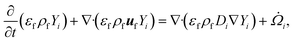
The volume-filtered continuity equation for a variable density, low Mach number flow is given by| | 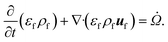 | (1) |
where εf, ρf, and uf are the fluid-phase volume fraction, density, and velocity, respectively. ![[capital Omega, Greek, dot above]](https://www.rsc.org/images/entities/i_char_e1bf.gif) is the volumetric rate of mass transfer from the devolatilizing biomass particles to the gas phase at a given point in space and time. The volume-filtered momentum equation is given by
is the volumetric rate of mass transfer from the devolatilizing biomass particles to the gas phase at a given point in space and time. The volume-filtered momentum equation is given by| | 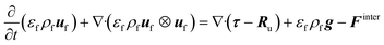 | (2) |
where g is the gravity vector and Finter represents the inter-phase momentum exchange between particles and the fluid. The volume-filtered fluid-phase stress tensor τ is expressed as| | 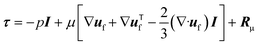 | (3) |
where I is the identity matrix and P and μ are the fluid pressure and dynamics viscosity, respectively. Rμ is a subfilter momentum flux accounting for enhanced dissipation due to the presence of the particles. Rμ is modeled using an effective viscosity model as| | 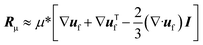 | (4) |
where μ* is the effective viscosity and for fluidized beds is given by28Another subfilter momentum flux Ru, similar to classical Reynolds stress, is modeled using an eddy viscosity model| | 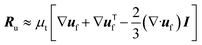 | (6) |
where μt is the turbulent viscosity computed via a dynamic Smagorinsky model29,30 based on Lagrangian averaging.31
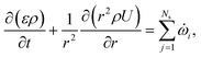
For a reaction scheme involving Ns gaseous species, the mass fraction Yi of the ith gaseous species is computed using the species conservation given by
| |  | (7) |
where 1 ≤
i ≤
Ns.
Di is the mass diffusivity and
i is the filtered chemical source term.
Eqn (7) represents a system of
Ns coupled PDEs, indicating an increase in computational complexity and cost with the increasing size of the reaction scheme used. Note that the secondary gas-phase reactions are not significant at the reactor temperature of 500 °C.
i appears in
eqn (7) due to the species transfer from biomass particles to the gas phase during devolatilization.
i depends on the particle-scale biomass devolatilization model used. An additional source term can be easily added to
eqn (7) in case gas-phase homogeneous reactions are present, for example, during biomass gasification.
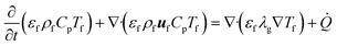
The enthalpy conservation equation to calculate the gas-phase temperature Tf is given by
| |  | (8) |
Here
Cp and
λg are the gas-phase specific heat capacity and thermal conductivity, respectively.
![[Q with combining dot above]](https://www.rsc.org/images/entities/i_char_0051_0307.gif)
is the enthalpy source term due to the heat transfer between the gas and the solid particles (sand and biomass) and the transfer of devolatilization products from biomass particles to the gas phase. Note that the subfilter convective and diffusive fluxes appearing in
eqn (7) and
(8) are neglected due to their limited contribution and the unavailability of appropriate closures.
32 This assumption is commonly employed in the literature.
4,32
2.1.2 Particle phase description.
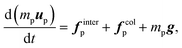
In the CFD–DEM framework, the solid phase (sand and biomass particles) is treated in a Lagrangian framework, where individual particle trajectories are solved using Newton's second law of motion. The equations of motion for the particles are given by| |  | (9) |
| |  | (10) |
and| | 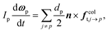 | (11) |
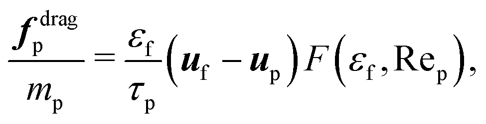
where xp is the position, up is the velocity, ωp is the angular velocity, mp is the mass, and Ip is the moment of inertia of particle p. Eqn (10) shows that a particle's trajectory is governed by three forces: finterp is the force exerted by the carrier fluid, mpg is the gravitational force, and fcolp is the collision force with adjacent particles and the walls. Collisions are handled via a soft-sphere approach originally proposed by Cundall and Strack.33 Particle rotation is assumed to be only a function of the tangential component of the collision force, fcolt, that is solved based on the Coulomb friction law. Further details can be found in ref. 27. finterp is given by| | | finterp ≈ Vp∇·τ + fdragp | (12) |
The first term on the right-hand side of eqn (12) represents contributions from the resolved fluid stresses and the second term accounts for the subfiltered stresses in the form of drag. The drag force depends on the gas-phase velocity uf and the fluid volume fraction εf at the particle location. These gas-phase variables are interpolated to the particle location via a second-order trilinear interpolation scheme. fdragp is calculated as| | 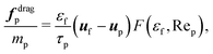 | (13) |
where τp = ρpd2p/(18μ) is the particle response time derived from Stokes flow with dp being the particle diameter. F is the dimensionless drag force coefficient of Tenneti et al.34 that depends on εf and the particle Reynolds number Rep given by| | 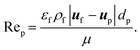 | (14) |
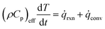
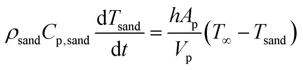
Sand particles are inert, whereas biomass particles undergo thermochemical conversion governed by solid-phase devolatilization reactions coupled with the intraparticle transport processes. The temperature change of sand particles is primarily due to the heat exchange with the gas phase.
| | 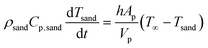 | (15) |
where
ρsand,
Cp,sand, and
Tsand are the density, specific heat capacity, and temperature of the sand particles. The RHS term is the convective heat transfer rate between gas and a particle per unit volume. Here,
T∞ is the ambient gas temperature evaluated at the particle location.
Ap and
Vp are the particle's surface area and volume, respectively.
h is the convective heat transfer coefficient and is calculated using Gunn's correlation.
35| | | Nu = (7 − 10εf + 5ε2f)(1 + 0.7Re0.2pPr0.33) + (1.33 − 2.4εf + 1.2ε2f)Re0.7pPr0.33 | (16) |
where Nu is the Nusselt number,
εf is the gas-phase volume fraction evaluated at the particle location, Re
p is the particle Reynolds number, and Pr is the Prandtl number.
The temperature of biomass particles depends on the heat transfer with the gas phase and the thermochemical conversion process. Modeling of a devolatilizing biomass particle is detailed next.
2.2 Biomass devolatilization models
This section presents the mathematical description of the intraparticle and homogeneous particle models. The thermochemical reactions of biomass devolatilization are represented by the multi-step mechanism developed by the CRECK modeling group.9 This kinetic model describes the devolatilization of five biomass constituents: cellulose, hemicellulose, and three types of lignin, involving ns = 19 solid species, Ns = 20 gas phase species, and 24 reactions. The kinetic model has been extensively validated against experiments.
2.2.1 Intraparticle model.
The intraparticle processes of the devolatilizing biomass are represented by a spherically symmetric one-dimensional model.8 Biomass properties, such as temperature and composition, are a function of both position and time. The intraparticle model8 has been rigorously validated against the experiments of Park et al.36 using uncertainty quantification. In the validation study, the temperature inside the particle, solid mass, and the lumped products are considered. For more details, the readers can refer to the previous work.8 A brief description of the governing equations and the boundary conditions of the intraparticle model is provided here.
Physicochemical processes occurring inside a devolatilizing biomass particle are represented by the conservation equations of mass, energy, and gas phase species along with a chemical kinetics mechanism.9 The resulting set of coupled non-linear governing equations is numerically solved to get the instantaneous spatially resolved state of the biomass particle.
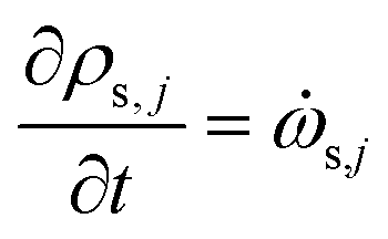
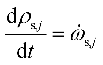
The rate of change of density of solid components is given by
| |  | (17) |
where
ρs,j is the density of solid component
j = 1 to
ns and
![[small omega, Greek, dot above]](https://www.rsc.org/images/entities/i_char_e15a.gif) s,j
s,j is the reaction source term for solid component
j obtained from the chemical kinetic scheme.
ns = 19 in this work. The continuity equation (mass conservation) is written as
| |  | (18) |
where
ε is the particle porosity,
ρ is the gas density,
U is the superficial velocity of the gas, and

is the net source term for gas phase species.
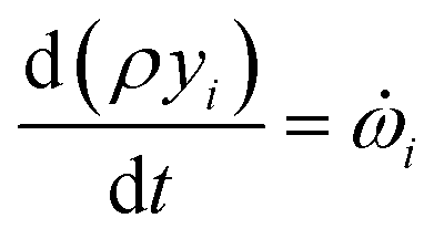
Ns = 20 in this work. The gas phase is assumed to be ideal. Particle porosity is assumed to be constant, while the particle diameter reduces with devolatilization. The species conservation equation is given by
| | 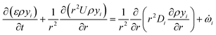 | (19) |
where
yi is the mass fraction,
Di is effective diffusivity, and
i is the source term of gas-phase species
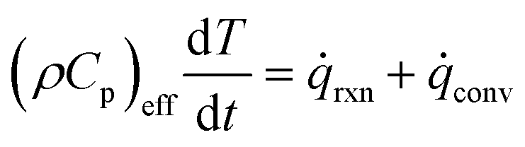
i. Assuming local thermal equilibrium between the gas and the solid phases, the energy conservation equation is given by
| | 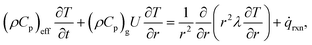 | (20) |
where
T is the particle temperature, (
ρCp)
eff is the combined heat capacity of the solid and gas phases at a given location inside the particle, (
ρCp)
g is the heat capacity of the gas phase at a given location inside the particle,
![[q with combining dot above]](https://www.rsc.org/images/entities/i_char_0071_0307.gif) rxn
rxn is the source term due to devolatilization reactions, and
λ is the effective thermal conductivity, calculated as the weighted sum of solid components and gas phase conductivity, including the effect of radiative heat transfer through pores.
37
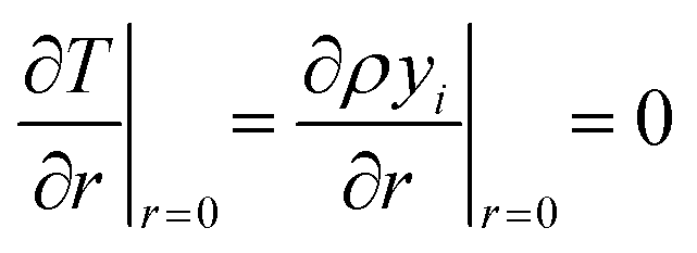
At the particle center, a zero gradient condition is imposed due to spherical symmetry.
| |  | (21) |
The contribution of particle–particle heat conduction in comparison to convection is considered minor in fluidized beds
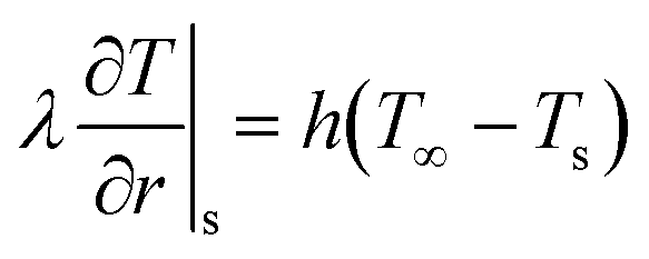
4,17,38,39 and neglected in this work. At the particle surface, species and heat flux are imposed by convective mass and heat transfer, respectively.
| | 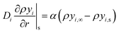 | (22) |
| | 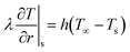 | (23) |
where
yi,s is the mass fraction of gas species
i at the particle surface,
yi,∞ is the ambient mass fraction of gas species
i,
Ts is the particle surface temperature, and
T∞ is the ambient temperature.
α and
h are the convective mass and heat transfer coefficients, respectively, and are calculated using Gunn's correlation (
eqn (16)). For
α calculation, the Prandtl number is replaced with the Schmidt number in Gunn's correlation, providing the Sherwood number.
2.2.2 Homogeneous particle model.
In the homogeneous model, particle evolution is assumed to be uniform in space (zero-dimensional) and is only a function of time.1,4 The governing equations of a homogeneous particle model are summarized here.
The rate of change of solid component density ρs,j for j = 1 to ns is given by
| |  | (24) |
where
s,j is the source term for solid component
j obtained from the chemical kinetic scheme. The rate of change of the gaseous species is given by
| |  | (25) |
where
yi and
i are the mass fraction and the source term for gas phase species
i, respectively. The temperature of the particle is evaluated using the overall energy balance
| |  | (26) |
where
T is the particle temperature, (
ρCp)
eff is the combined heat capacity of solid and gas phases, and
rxn is the source term due to the devolatilization reactions.
conv is the convective heat transfer rate, between gas and a particle, per unit volume given by
| |  | (27) |
Here,
T∞ is the ambient temperature, and
Ap and
Vp are the particle's surface area and volume, respectively.
h is the convective heat transfer coefficient and is calculated using Gunn's correlation
35 (
eqn (16)).
2.3 Interphase coupling
Coupling between the gas phase and solid particles appears in the form of the fluid volume fraction εf and the interphase exchange terms for momentum Finter, mass , chemical species i, and heat . These interphase exchange terms appear as source terms in the volume-filtered conservation equations for the gas phase described in section 2.1.1. Details of these interphase coupling terms are provided here.
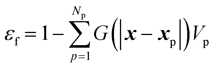
The fluid volume fraction is calculated as
| | 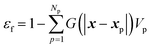 | (28) |
where
Np is the number of particles (biomass and sand).
G is the filtering kernel considered to be Gaussian with a characteristic length scale
δf, defined as the width at half the kernel height. Here,
δf = 7
dp,
i.e., seven times the mean particle diameter, is considered.
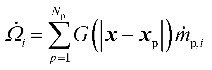
The interphase mass transfer of gas species i (from biomass particles to gas) is given as
| | 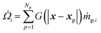 | (29) |
where
ṁp,i is the instantaneous production rate of species
i during devolatilization of biomass particle
p.
ṁp,i is calculated by multiplying
eqn (22) (species flux from the particle surface) with
Ap in case of the intraparticle model. For the homogeneous model,
ṁp,i is calculated from
eqn (25) (volumetric species source) by multiplying it with
Vp.
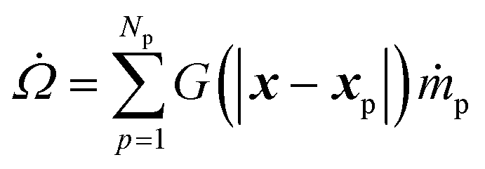
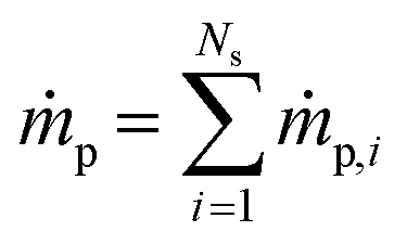
The interphase mass transfer (from biomass particles to gas) is given as
| |  | (30) |
where

is the net rate of production of the gaseous species during devolatilization of biomass particle
p.
The momentum exchange is defined as
| |  | (31) |
Here
upṁp represents the momentum addition to the gas phase from biomass devolatilization products.
The interphase heat transfer is calculated as
| |  | (32) |
where
inter is the rate of heat transfer between gas and solids and is calculated using
eqn (23) multiplied with
Ap and
eqn (27) multiplied with
Vp for the intraparticle and homogeneous models, respectively.
ṁpCp,effT represents the enthalpy addition to the gas phase from biomass devolatilization products.
The numerical implementation of these exchange terms requires extrapolation of the particle data to the computational mesh. This implementation is performed in two steps to make it computationally efficient.27 First, the particle data are extrapolated to the nearest neighboring mesh. In the second step, the extrapolated data are then diffused implicitly such that the final width of the filtering kernel is tied to the selected filter size δf.
2.4 Numerical implementation
The volume-filtered variable density equations introduced in section 2.1 are implemented in the framework of NGA,26 a fully conservative CFD code tailored for reacting turbulent multiphase flow computations. The Navier–Stokes equations are solved on a staggered grid with second-order spatial accuracy for both the convective and the viscous terms, and the second-order accurate semi-implicit Crank–Nicolson scheme40 is implemented for time advancement. The details on the mass, momentum, and energy-conserving finite difference scheme are available in ref. 26. The fluidized bed reactor is modeled as a vertical pipe with inlet and outlet boundary conditions. To account for the cylindrical geometry on a Cartesian mesh, a conservative immersed boundary (IB) method, based on a cut-cell formulation,41 is employed.
The particles are distributed among the processors based on the underlying domain decomposition of the gas phase. For each particle, its position, velocity, and angular velocity are solved using a second-order Runge–Kutta scheme. To properly resolve the collisions without requiring an excessively small timestep, particles are restricted to move no more than one-tenth of their diameter per timestep.
The coupled nonlinear partial differential equations (PDEs) of the intraparticle devolatilization model (see section 2.2) are discretized using finite differences. The central difference scheme is used for the diffusion terms and an upwind scheme is used for the convective terms. The temporal terms are discretized using the backward Euler implicit scheme. The resulting tridiagonal system is solved using the Thomas algorithm. At each timestep, all the discretized equations are solved iteratively until a converged solution is obtained. DVODE,42 an open-source stiff ODE solver, is used to accurately and efficiently evaluate the chemical source terms in eqn (17), (18), (24), and (25).
3 Model assessment
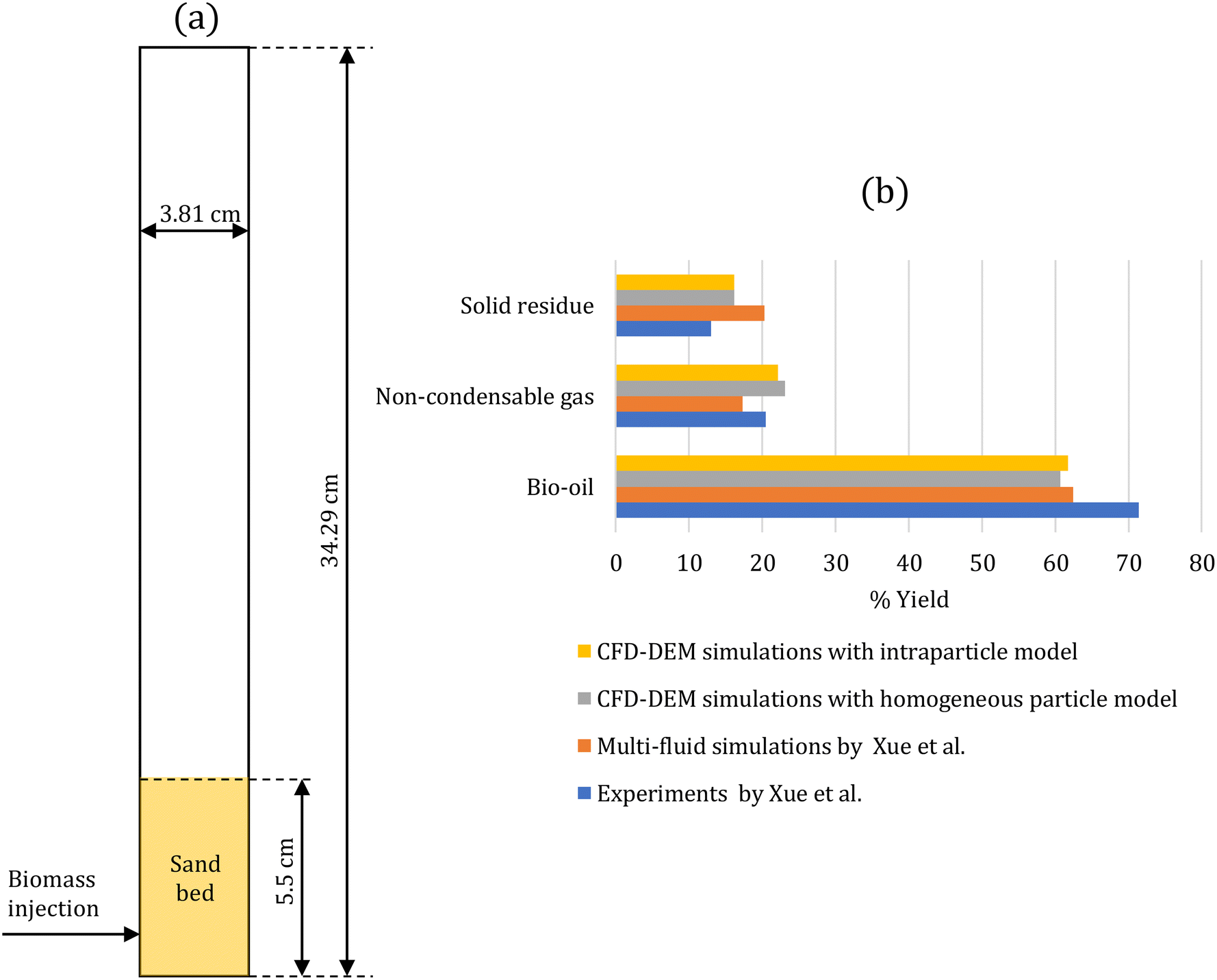
The developed multiscale computational framework is assessed against the experiments of biomass pyrolysis in a fluidized bed at 500 °C performed by Xue et al.43 This setup has been used for assessment by several simulation studies.43–47Fig. 1a shows the two-dimensional geometry of the fluidized bed reactor simulated to represent the experimental set-up. Table 1 provides the simulation parameters. A cold flow simulation is initially performed with sand particles until steady fluidization is achieved. Consequently, biomass (red oak) particles are continuously injected into the bed to simulate biomass pyrolysis. These simulations are performed using the intraparticle (see section 2.2.1) and homogeneous (see section 2.2.2) models for biomass devolatilization. The biomass feed rate is scaled to maintain the same ratio of the biomass feed rate to the gas flow rate as in the experiments. The simulations are performed for 20 s to ensure that the outlet mass fraction of gas-phase species reaches a statistical steady state.
 |
| | Fig. 1 (a) Two-dimensional fluidized bed reactor geometry of the experimental setup43 used for the assessment of the multiscale CFD–DEM simulations; (b) % yield of condensable species (bio-oil), non-condensable species (gas), and solid residue at the reactor outlet obtained from the CFD–DEM simulations with homogeneous and intraparticle models, and the simulations and experiments by Xue et al.43 Experimental error is reported to be ±1.4, ±1.5, and ±1.3 for the yields of bio-oil, solid residue, and non-condensable gases, respectively.43 | |
Table 1 CFD–DEM simulation parameters for the model assessment
| Parameter |
Value |
| Fluidized bed length |
0.343 m |
| Fluidized bed width |
0.038 m |
| Fluidized bed depth |
0.001 m |
| Cells along length |
343 |
| Cells along width |
38 |
| Cells along depth |
1 |
| Number of sand particles |
16![[thin space (1/6-em)]](https://www.rsc.org/images/entities/char_2009.gif) 280 280 |
| Biomass type |
Red oak |
| Biomass composition |
Cellulose: 0.41 |
| Hemicellulose: 0.32 |
| Lignin: 0.27 |
| Biomass injection rate |
2.67 × 10⁻⁷ kg s−1 |
| Biomass injection height |
1.7 cm |
| Size of sand particles |
520 μm |
| Size of biomass particles |
325 μm |
After reaching a statistical steady state, the gas-phase species mass fraction at the reactor outlet is time-averaged over 3 s with an interval of 0.1 s and spatial-averaged over the reactor cross section. Fig. S5 in the ESI† shows that 3 s is a sufficient time period to obtain time-averaged data. Species such as glyoxal, HMFU, H2O, levoglucosan (LVG), methanol, ethanol, xylose, C11H12O4, and HCOOH are classified as condensable species as they are liquids at room temperature. The remaining gas-phase species, such as CO and H2, are classified as non-condensable gases. Fig. 1b compares the % yield of condensable species (bio-oil), non-condensable species (gas), and solid residue at the reactor outlet predicted by the CFD–DEM simulations and the experimental measurements and simulation of Xue et al.43 The literature simulation studies43–47 predict bio-oil, gas, and char in the range of 61–77%, 14–17%, and 7–22%, respectively. The experimental error for bio-oil, solid residue, and non-condensable gases yields is ±1.4, ±1.5, and ±1.3, respectively,43 much lower than the differences between the simulation predictions and experimental measurements. The differences between the simulations and experiments are attributed to the underlying kinetic model used in the CFD simulations.44 Our simulation predictions for tar and char are in this range. In contrast, the gas predictions are higher than those in the literature studies and closer to the experimental measurements. These results further underscore the role of the kinetic model in reactor-scale simulations. The impact of particle-scale models (homogeneous and intraparticle models) on the simulation predictions is minor as the biomass Biot number is small (Bi = 0.36).
4 Time scales
Gas residence time tg, biomass devolatilization time td, and solid circulation time tc play an essential role in understanding the coupling between particle and reactor-scale processes during biomass pyrolysis in a fluidized bed reactor. This section details the calculation of these time scales.
Gas residence time tg is calculated as the ratio of expanded bed height to the mean superficial velocity in the bed. Both of these parameters are obtained from the CFD–DEM simulations. Biomass devolatilization time td is the characteristic time scale associated with the thermochemical conversion of biomass during devolatilization. td is obtained by performing single particle biomass devolatilization simulations using the homogeneous and intraparticle models. Average values of the heat and mass transfer coefficients experienced by biomass particles in the CFD–DEM simulations of a fluidized bed are used in the convective heat and mass transfer boundary conditions for the single particle simulations.
Solid circulation time or solid mixing time tc is the time scale associated with the mixing of solid particles in a fluidized bed. tc determines the time needed for a particle to circulate from the bottom of the bed to reach its initial position.48 The particle trajectory data obtained from the CFD–DEM simulation is used to evaluate tc. To this end, the time taken by several randomly selected particles to traverse through the bed and reach the initial point is evaluated. More details about the calculation of tc is provided in section S1 of the ESI.†
In the literature, tc is also commonly calculated using empirical correlations.49 The following correlation50 based on the expanded bed height H, bubble rising velocity Ub, inlet gas velocity Uin, and minimum fluidization velocity Umf is used to estimate tc.
| |  | (33) |
The impact of reactor size on these time scales is discussed in section S1 in the ESI.
†
5 Multiscale CFD–DEM simulations of biomass pyrolysis
CFD–DEM simulations of biomass pyrolysis at 500 °C are performed in a three-dimensional bubbling fluidized bed using the intraparticle (see section 2.2.1) and homogeneous (see section 2.2.2) biomass devolatilization models. The computational domain corresponds to the commonly studied micro fluidized bed reactor.51Fig. 2 shows the simulation setup and Table 2 provides the simulation parameters. Biomass particle size and thermal conductivity are varied to obtain two Biot numbers, Bi: 0.26 and 1.6. Bi is defined as the ratio of the conductive heat transfer resistance within a particle to the convective heat transfer resistance outside the particle. Small Bi implies a uniform temperature within the particle, whereas O(1) and greater values correspond to significant temperature variation in the particle.
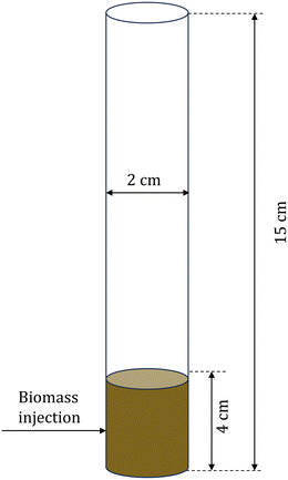 |
| | Fig. 2 Schematic of the computational domain for the multiscale CFD–DEM simulations of biomass pyrolysis in a fluidized bed reactor. | |
Table 2 Parameters for the three-dimensional CFD–DEM simulations of biomass pyrolysis in a fluidized bed
| Parameter |
Value |
| Fluidized bed height |
15 cm |
| Fluidized bed diameter |
2 cm |
| Cells along height |
75 |
| Cells along width |
10 |
| Cells along depth |
10 |
| Sand particle diameter |
500 microns |
| Sand particle density |
2600 kg m−3 |
| Number of sand particles |
110840 |
| Biomass type |
Poplar wood |
| Biomass composition |
Cellulose: 0.4806 |
| Hemicellulose: 0.2611 |
| C-rich lignin: 0.0214 |
| H-rich lignin: 0.0957 |
| O-rich lignin: 0.1325 |
| Ash: 0.0086 |
| Biomass particle diameter |
500 μm (Bi = 0.26) |
| 1.5 mm (Bi = 1.6) |
| Biomass injection rate |
7.34 × 10⁻⁶ kg s−1 |
| Restitution coefficient |
0.8 |
| Friction coefficient |
0.092 |
| Inlet gas velocity |
0.35 m s−1 (= 3Umf) |
In CFD–DEM simulations, the grid size primarily depends on the particle diameter and should be bigger than the largest particle. The grid size is varied from dp to 4dp, where dp = 500 μm is the sand size. In this range, no significant impact on the reactor behavior was observed. A uniform grid size of 4dp is used in the simulations to ensure that the grid size is about 1.33 times the largest biomass particle (1.5 mm). Section S2 of the ESI† provides more details about the grid convergence study. In the CFD–DEM simulations using the intraparticle model, twenty grid points are found to be sufficient to resolve each biomass particle. Section S3 of the ESI† provides more details of the particle-scale grid convergence study. The following subsections discuss the evolution of individual biomass particles and the overall reactor dynamics during the simulations of biomass pyrolysis in the fluidized bed.
5.1 Particle-scale analysis
In the CFD–DEM simulations, biomass particles are continuously injected into the reactor, reaching a maximum of 500 and 2000 for the high and low Bi, respectively. Properties such as temperature, composition, species production rates, and size of each biomass particle are tracked. The evolution of one biomass particle in the CFD–DEM simulations using both particle models is analyzed and reported here. We ensured that the selected biomass particle was injected simultaneously in the CFD–DEM simulations using the homogeneous and intraparticle model. Fig. 3 shows the biomass particle position and the particle velocities at different time instants for high Bi. A clear distinction can be observed in the simulation predictions based on the homogeneous (top row) and intraparticle (bottom row) models. This impact of particle-scale models on bed hydrodynamics is attributed to the differences in the production rate of devolatilization products. The species production rate is faster for the homogeneous model than for the intraparticle model. The release of species from a biomass particle to the surroundings impacts the local flow field, changing the bed dynamics. More details about the production rates are provided in the discussion of Fig. 5. For low Bi (Bi = 0.26), the profiles within the particle obtained from the intraparticle and homogeneous models are similar. Thus, the low Bi case is not discussed here.
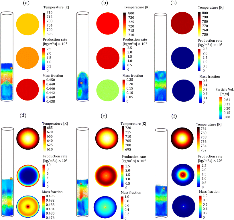 |
| | Fig. 3 Particle velocity distribution obtained from the CFD–DEM simulations of biomass pyrolysis with homogeneous (top row) and intraparticle (bottom row) models. The evolution of about O(103) biomass particles is tracked in the CFD–DEM simulations. The insights into the conversion of a specific biomass particle (orange circle inside the fluidized bed geometry) injected simultaneously in both particle model based CFD–DEM simulations are highlighted. The profiles of temperature, LVG production rate, and cellulose mass fraction within the biomass particle are provided at 30% (a and d), 60% (b and e), and 90% (c and f) of the devolatilization time td. | |
Fig. 3 also shows the colormaps of the temperature, LVG production rates, and cellulose mass fraction within the biomass particle at 30% (t1), 60% (t2), and 90% (t3) of the devolatilization time td. As expected, the homogeneous model shows a uniform distribution as this model is only a function of time. In contrast, the intraparticle model shows significant variations within the particle. A quantitative comparison of these intraparticle profiles is shown in Fig. 4. For instance, a higher temperature at the particle surface than at the center can be seen in the intraparticle model (see Fig. 4a). This variation reduces as the devolatilization progresses. However, temperature predictions of the homogeneous model are always higher than those of the intraparticle model, indicating faster biomass heating in the homogeneous model. The uniform heat distribution in the homogeneous model makes the temperature differential between the gas and particles higher than that in the intraparticle model, leading to faster heating.
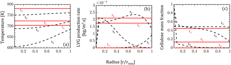 |
| | Fig. 4 Profiles of (a) temperature, (b) levoglucosan (LVG) production rate, and (c) cellulose mass fraction within a single biomass particle in the fluidized bed at 30% (t1), 60% (t2), and 90% (t3) of devolatilizing time td. The data are obtained from the CFD–DEM simulations of biomass pyrolysis in a fluidized bed with homogeneous (solid red lines) and intraparticle models (dashed black lines). Twenty grid points are used to resolve the biomass particle in the intraparticle model. | |
The intraparticle model predicts the peak LVG production rate shifting from the particle surface to the center as devolatilization progresses (see Fig. 4b). Such peaks are not observed in the corresponding temperature profiles. The LVG production rate profile depends on the distribution of the temperature and biomass composition. The intraparticle model shows a progressive cellulose conversion from the particle surface toward the center (see Fig. 4c). These results illustrate that the devolatilization process significantly varies within biomass particles at high Bi (Bi = 1.6), and the homogeneous model fails to capture these variations.
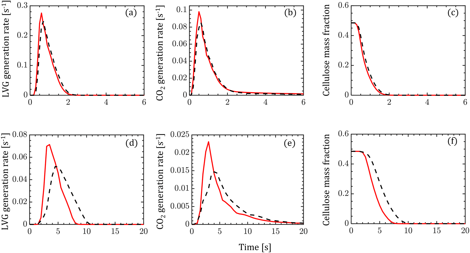
The transient evolution of LVG and CO2 production rates and cellulose mass fraction integrated over a biomass particle are analyzed. Fig. 5 compares these transient profiles obtained from the homogeneous (solid red lines) and intraparticle (dashed black lines) models at low Bi (top row of Fig. 5) and high Bi (bottom row of Fig. 5). Both the particle models show similar predictions at low Bi, whereas at high Bi, the homogeneous model predicts faster release of LVG and CO2 and cellulose decomposition rate than the intraparticle model. For high Bi, the production rate curves predicted by the homogeneous model are narrower and shift to an earlier time than the intraparticle model predictions. The faster heating of biomass can explain these observations in the case of the homogeneous model than in the intraparticle model.
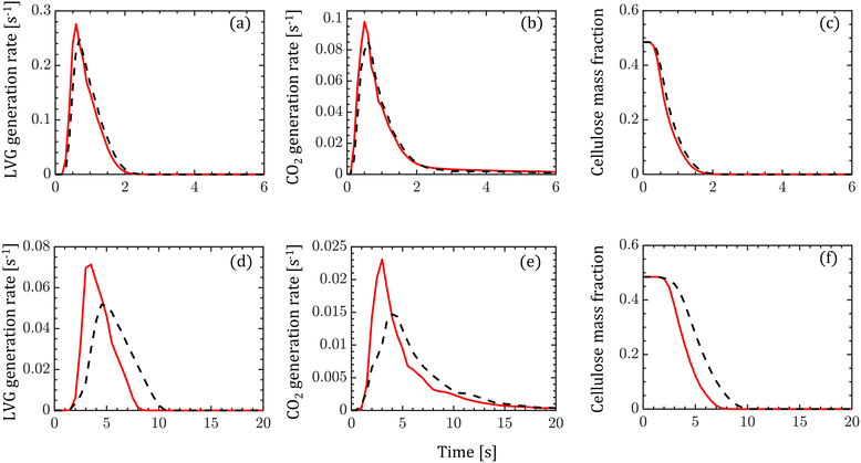 |
| | Fig. 5 Time evolution of a single biomass particle during the simulations of biomass pyrolysis in the fluidized bed. Red solid lines: homogeneous model; black dashed lines: intraparticle model. Top row: Low Bi case; bottom row: high Bi case. (a and d) LVG production rate; (b and e) CO2 production rate; (c and f) cellulose mass fraction. | |
Despite the significant differences between the particle-scale models' predictions of the intraparticle profiles and transient evolution at high Bi, the difference between the species yield predictions is less than 5%. The maximum difference is 4% for xylose among the condensable and 4.2% for CO among the permanent gases. To understand this behavior, the impact of biomass heating rate on the species production rates and yields is analyzed. Devolatilization of a single biomass particle is simulated using the homogeneous model at three constant heating rates: 50, 100, and 1500 K s−1 until the particle temperature reaches 773 K. Fig. 6a and b show the evolution of the biomass temperature and LVG production rate, respectively. As the heating rate increases, the production peak increases and the time to reach the peak decreases. This observation demonstrates the strong sensitivity of the production rate and peak production time on the heating rate. In contrast, the species yields are insensitive to the heating rate at higher values (>100 K s−1) and are mildly sensitive at smaller values (<100 K s−1) as shown in Fig. 6c. Experimental investigations have reported a negligible impact of particle size on the product yield, implying the negligible impact of Bi.52
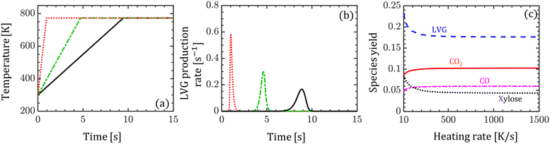 |
| | Fig. 6 Sensitivity of biomass devolatilization to the heating rate. (a) Particle temperature variation with time at different heating rates: red dotted line (1500 K s−1), green dash-dotted line (100 K s−1), black solid line (50 K s−1); (b) production rate of LVG at different heating rates: red solid line (1500 K s−1), green dash-dotted line (100 K s−1), black dashed line (50 K s−1); (c) species (LVG, CO2, CO, and xylose) yields as a function of the heating rate. | |
These results explain the particle-scale behavior observed in the fluidized bed simulations. The heating rate of O(1) mm biomass particles is high in fluidized beds, making the species yield insensitive to the particle models. For low Bi, the average heating rate of homogeneous and intraparticle models is 1288 K s−1 and 1076 K s−1, respectively. For high Bi, these values reduce to 135 K s−1 and 62 K s−1, respectively. For both Bi, the intraparticle model predicts a heating rate which is maximum near the surface and minimum near the center. At high Bi, although intraparticle profiles differ significantly between the particle-scale models, relatively high heating rates O(100) K s−1 lead to small variations (up to 5%) in the species yields.
At any instant, biomass particles exist at different devolatilization stages in the fluidized bed. Fig. 7 shows the distribution of biomass properties: temperature (Fig. 7a and d), LVG production rate (Fig. 7b and e), and cellulose mass % (Fig. 7c and f) for low Bi (top row) and high Bi (bottom row) at 6.5 s (0.5td) of the simulation time. For low Bi, a small difference is observed between the particle-scale models as expected. However, at high Bi, significant differences are observed in the distribution. The intraparticle model predicts a relatively cooler core of biomass particles than the homogeneous model, implying lower progress in devolatilization (Fig. 7d). The lower temperature in the intraparticle model case leads to a higher fraction of biomass particles having a lower LVG production rate (Fig. 7e) and a higher unconverted cellulose content (Fig. 7f).
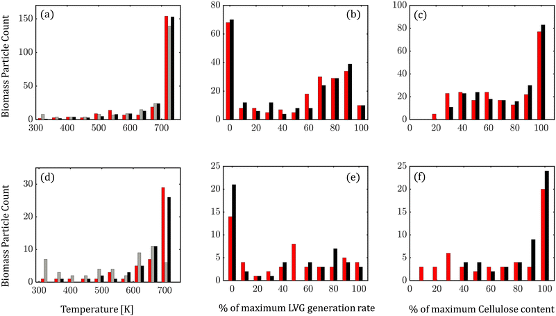 |
| | Fig. 7 Distribution of biomass properties in the multiscale CFD–DEM fluidized bed simulations at 50% of the biomass devolatilization time. Top row: Low Bi; bottom row: high Bi. (a and d) Biomass temperature, red: homogeneous model predictions, black: intraparticle model predictions at the particle surface, grey: intraparticle model predictions at the particle center; (b and e) LVG production rate, red: homogeneous model predictions, black: intraparticle model predictions; (c and f) cellulose content, red: homogeneous model predictions, black: intraparticle model predictions. | |
5.2 Reactor-scale analysis
This subsection describes the impact of particle-scale models on the reactor-scale dynamics, i.e., the evolution of pyrolysis products in the fluidized bed reactor. Table 3 provides the time scales associated with the multiscale CFD–DEM simulations of biomass pyrolysis. For both low and high Bi, the gas residence time, tg = 0.13 s, is at least an order of magnitude lower than the devolatilization time td and solid circulation tc = 14 s time. tc estimated from the simulation (1.4 s) is close to the value evaluated from the standard correlations (∼1 s) summarized in section 4. tg ≪ tc implies that the devolatilization products released from biomass particles quickly escape the fluidized bed without rigorous mixing in the multiphase region. In the literature, the multiphase region is commonly treated as perfectly mixed and modeled as a CSTR.49,53 The time-scale analysis shows that this assumption is not always true and should be evaluated after considering the gas residence time. The remaining part of this subsection first discusses the time-averaged species compositions at the reactor outlet. Subsequently, the evolution of major product species within the reactor is analyzed.
Table 3 Time scales associated with biomass pyrolysis in the fluidized bed reactor
| Time scale |
Value |
| Solid mixing time, tc |
1.4 s |
| Gas residence time, tg |
0.13 s |
| Devolatilization time, td (low Bi) |
1.8 s (homogeneous) |
| 1.9 s (intraparticle) |
| Devolatilization time, td (high Bi) |
10.6 s (homogeneous) |
| 13.2 s (intraparticle) |
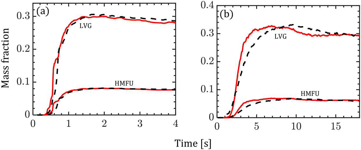
Fig. 8 shows the normalized mass fraction of the major volatile species (LVG and HMFU) at the reactor outlet. At low Bi, both homogeneous and intraparticle model predictions are almost identical as shown in Fig. 8a. In contrast, Fig. 8b shows faster release of the volatile species by the homogeneous model (peak at ∼6 s) than the intraparticle model (peak at ∼9 s) at high Bi. The normalized mass fractions of LVG and HMFU at the reactor outlet are time-averaged for the last 3 s of the simulation time with an interval of 0.2 s. The predictions based on both the particle models show less than 5% variation. The outlet product evolution approximately follows the particle-scale evolution as tg ≪ tc.
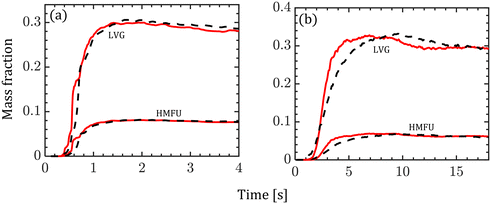 |
| | Fig. 8 Variation in the normalized mass fraction of LVG and HMFU at the reactor outlet (red solid line: homogeneous model; black dashed line: intraparticle model). (a) Low Bi case; (b) high Bi case. | |
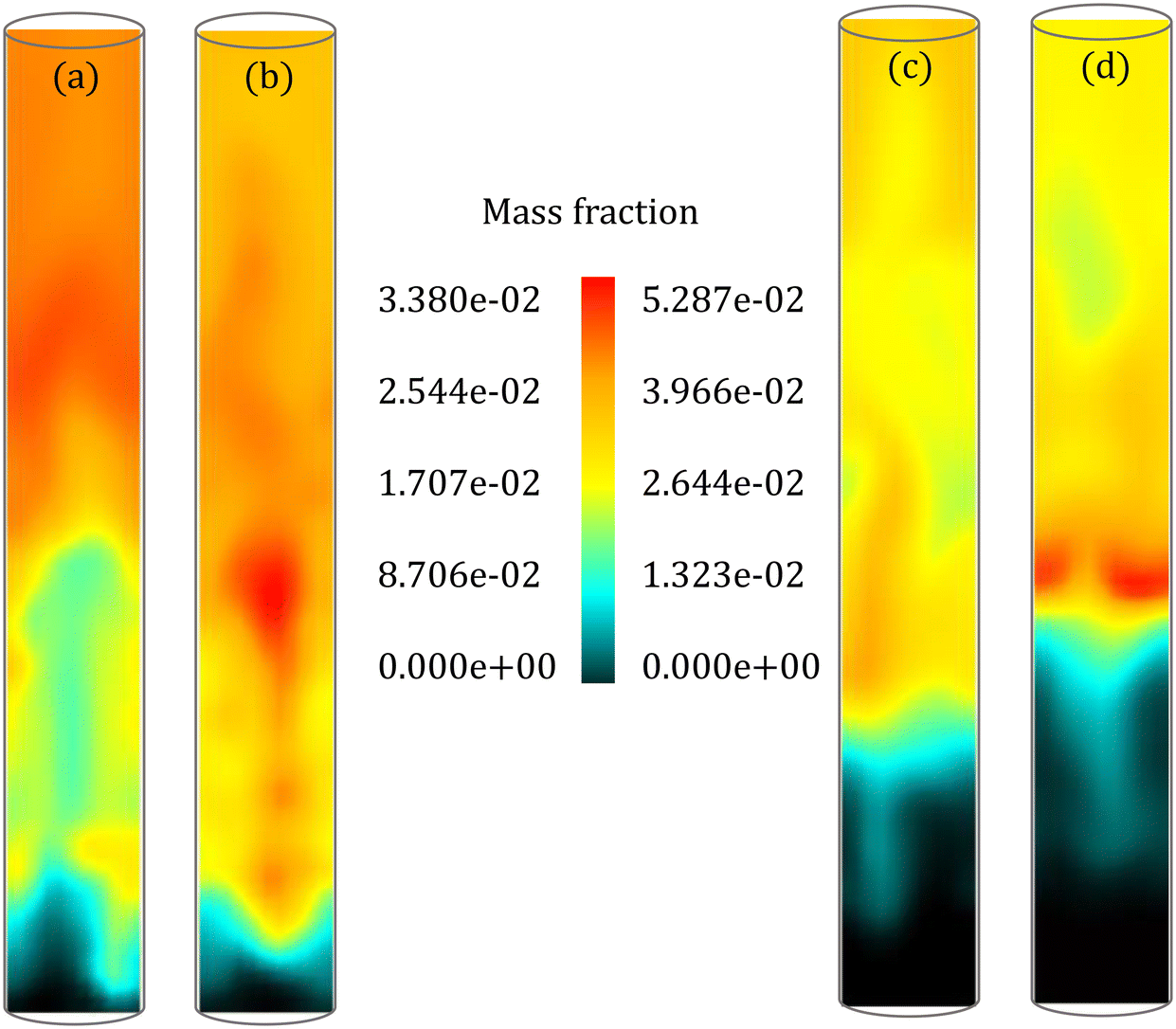
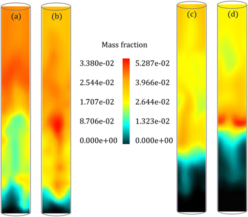
The instantaneous distribution of species mass fraction within the reactor allows a comparison of spatial variations in the species composition. Fig. 9 shows the LVG mass fraction within the reactor for low and high Bi at 7 s and 25 s, respectively. These results are obtained at a cross section passing through the reactor center after the simulations reached a statistical steady state. Although the average LVG mass fraction at the outlet predicted by the particle-scale models is similar (see Fig. 8), the instantaneous LVG distribution within the reactor is distinct. Even for low Bi, the colormap shows differences in the species composition distribution within the bed region (Fig. 9a and b). A similar behavior is observed at other time stamps. Fig. S6 and S7 in the ESI† provide instantaneous LVG composition profiles at other time stamps. However, the difference in the time-averaged profiles obtained from both particle-scale models is negligible as shown in Fig. S8 in the ESI.† This observation demonstrates that small particle-scale differences could lead to significant variations at the reactor scale. Such species non-uniformity in the bed region is observed for other gas-phase species too. However, the coefficient of variation (CV), defined as the ratio of the standard deviation to the mean, for all the species in the multiphase region is approximately 0.6 for both the particle-scale models with a maximum difference of ∼5%. This CV value suggests that significant non-uniformity in the species distribution is present in the multiphase region.
 |
| | Fig. 9 Instantaneous LVG mass fraction at a cross-sectional plane passing through the reactor center. Predictions of the (a) homogeneous model and (b) intraparticle model at 7 s for low Bi. Predictions of the (c) homogeneous model (d) intraparticle model at 25 s for high Bi. | |
For high Bi (Fig. 9c and d), the species composition obtained from the particle-scale models differs in both the multiphase and the freeboard regions. The CV for most species in the multiphase region is around 0.9 for both the particle-scale models with a maximum difference of ∼13%. The CV value demonstrates larger non-uniformity in the species distribution compared to the low Bi case (CV ∼ 0.6). This observation is linked to a larger td for high Bi than low Bi. A high value of td implies that the biomass particle spans a larger region of the bed during its devolatilization, enhancing the variations in the species composition. These results show that the particle-scale models impact not only the instantaneous distribution but also the statistics of the species composition in the fluidized bed.
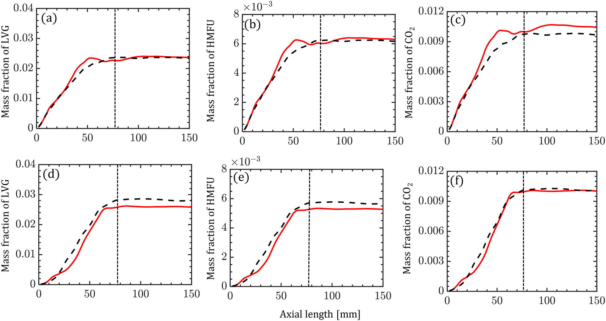
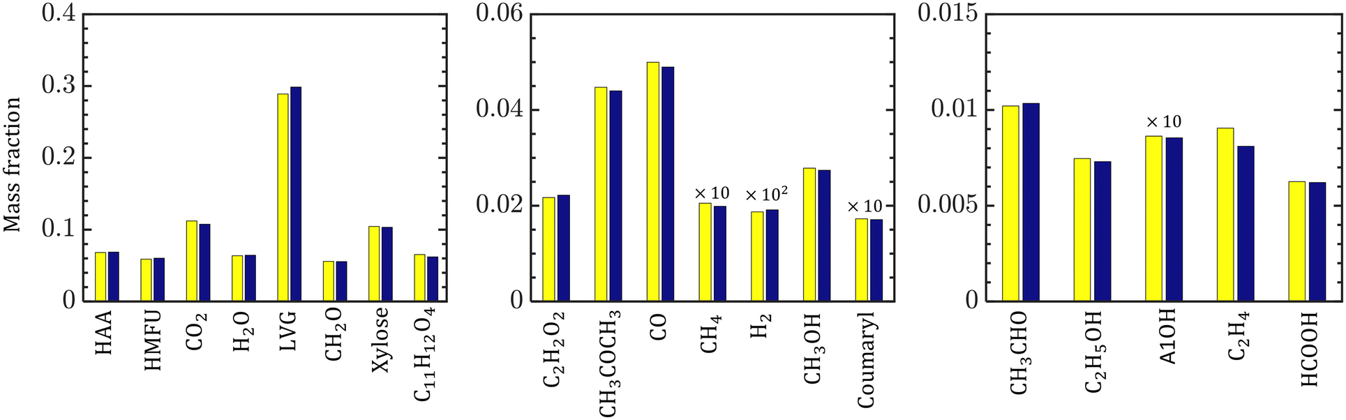
The species compositions are time-averaged (for 3 s with an interval of 0.2 s), and cross section averaged to obtain species composition variation along the reactor length. Fig. 10 compares the spatiotemporal averaged profiles of LVG, HMFU, and CO2 mass fraction for homogeneous (solid red lines) and intraparticle (dashed black lines) models at low Bi (top row) and high Bi (bottom row). As discussed earlier, significant non-uniformity in the species composition can be observed in the multiphase region. For all the cases, the species mass fraction almost linearly increases from the bottom of the bed to the expanded sand bed region. However, a significant difference between the predictions with different particle models is not observed. This trend is observed for all the devolatilization product species. Fig. 11 shows the mass fractions at the reactor outlet for all the twenty product species at high Bi. Minor variations are observed in the outlet species composition predicted using different particle-scale models.
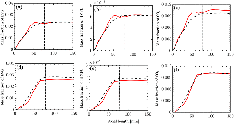 |
| | Fig. 10 Cross-sectional averaged species composition along the reactor length. The vertical dotted black line shows the expanded bed height; dashed black line: intraparticle model; solid red line: homogeneous model. Top row: Low Bi case, bottom row: high Bi case. (a and d) Mass fraction of LVG; (b and e) mass fraction of HMFU; (c and f) mass fraction of CO2. | |
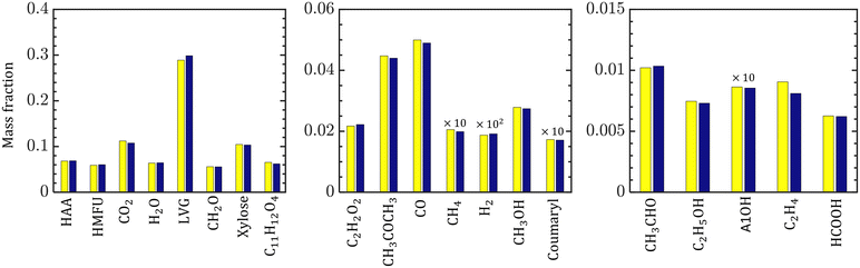 |
| | Fig. 11 Mass fraction of product species at the reactor outlet for the high Bi case. Mass fraction of CH4, coumaryl, and A1OH (oxygenated aromatics) are scaled by a factor of ten, and H2 mass fraction is multiplied by a hundred. Yellow and blue bars represent the predictions from the homogeneous and intraparticle models, respectively. | |
These results show that the averaged profiles are similar for both the particle models at low and high Bi. However, the instantaneous species distribution varies significantly within the bed. We anticipate particle-scale models to play a critical role at high reactor temperatures (>800 °C), where secondary gas phase reactions are significant. In such a case, spatiotemporal variations in the species composition within the reactor could significantly impact the gas phase reactions, leading to differences in the outlet composition too.
6 Computational expenses
All the CFD–DEM simulations are performed on the Param Shivay supercomputer (using 2× Intel Xeon Skylake 6148 processors) housed at IIT BHU. Simulating the cold flow fluidized bed simulations required ∼0.21 s on 36 cores for each timestep of 10 μs. The total simulation time is 12 hours, equivalent to 432 CPU hours, to achieve the bubbling fluidization regime. The multiscale CFD–DEM simulations of biomass pyrolysis in the fluidized bed for both homogeneous and intraparticle models required a smaller timestep of 5 μs to achieve convergence. Moreover, these simulations required approximately 550 hours on 40 cores, equivalent to 22000 CPU hours, to achieve statistical steady-state results.
The number of biomass particles steadily increases in the computational domain as a constant biomass feed rate is used. For low and high Bi, the maximum number of biomass particles is around 2000 and 500, respectively, whereas the number of sand particles is around 1.1 × 10⁵. The simulation time per timestep of the CFD–DEM simulations with a single biomass particle is approximately 0.29 s. Solving particle–particle collisions is the major simulation cost, constituting around 60% of the simulation time, followed by species conservation and pressure solvers, each contributing around 10% to the total time. For the maximum number of biomass particles considered (2000 particles), the time required to solve the homogeneous model is negligible compared to the other components of the CFD–DEM simulations. Thus, the simulation time per timestep remains almost constant for the homogeneous model even though the number of biomass particles increased.
In contrast to the homogeneous model, the CFD–DEM simulation time per timestep increases steadily from 0.29 s (1 biomass particle) to 0.35 s (2000 biomass particles) while using the intraparticle model. This increase in the simulation cost is primarily attributed to solving the governing equations (a set of coupled PDEs) of the intraparticle model within spatially resolved biomass particles (∼55% contribution) and the inter-processor communication cost of the data stored for biomass particles (∼45% contribution). Twenty-two standard variables, such as position, velocity, and temperature, are stored for each sand and biomass particle. In addition, 47 and 912 variables are stored for a biomass particle in the homogeneous and intraparticle models, respectively. The data stored in the intraparticle model is high as the variables are stored at twenty grid points within a biomass particle. Different data structures are used for sand and the homogeneous and intraparticle models to minimize the inter-processor communication cost. Using the same data structure for each particle type could make the CFD–DEM simulations prohibitive.
This analysis shows that coupling a one-dimensional description of particle-scale biomass devolatilization with CFD–DEM is not limited by the computational cost. For general fluidized bed simulations with a large number of inert particles, an adequate description of reacting particles, such as coal and catalyst, can be included without affecting the simulation time. The primary challenge lies in handling the complexity of the solver development.
7 Conclusions
The effect of particle-scale models, homogeneous and intraparticle, on CFD–DEM simulations of biomass fast pyrolysis in fluidized bed reactors is investigated. The homogeneous model neglects the spatial variations and the intraparticle model resolves the coupled reaction-transport processes within a biomass particle. Both models use a multistep kinetic scheme consisting of 24 reactions, 19 solid species, and 20 gas species. Significant spatial variations in the temperature, species production rates, and composition are observed within biomass particles at high Biot numbers. These spatial variations cannot be captured by the commonly used homogeneous model. Overall, the homogeneous model predicts rapid heating of biomass particles, resulting in a quicker release of devolatilization products than the intraparticle model. Despite these significant differences, the species yields differ by less than 5%. The sensitivity analysis shows that intraparticle processes have a negligible impact on species yields above the heating rate of 100 K s−1, which is common in fluidized beds.
The predictions of species mass fractions at the reactor outlet follow the variations observed at the particle scale. The species mass fractions at the reactor outlet predicted with both particle models differ by less than 5%. However, significant variations exist within the reactor. This observation is attributed to much smaller gas residence time than the solid circulation time, leading to significant non-uniformity in the sand bed region. This result challenges the common assumption of treating the bubbling bed region as a CSTR. The intra-reactor variations could impact the product composition in the presence of secondary gas-phase reactions that are significant at high reactor temperatures.
The computational cost of CFD–DEM simulations is dominated by particle collisions as the number of inert sand particles is much higher than biomass particles. The computational requirement for both particle-scale models is similar up to O(100) biomass particles. The CFD–DEM simulation time per timestep for the homogeneous model remained independent of the number of biomass particles. However, the simulation cost using the intraparticle model increased by ∼20% when the number of biomass particles increased to 2000. This increase in cost is attributed to solving the governing equations (a set of coupled PDEs) of the intraparticle model and the inter-processor communication of the data stored for biomass particles. The simulation cost is expected to grow with further mesh refining. A one-dimensional particle-scale model is appropriate for reactive CFD–DEM simulations as it does not significantly increase the simulation cost.
Data availability
The authors will provide the data upon request.
Conflicts of interest
The authors have no known conflicting financial interests that could potentially influence this work.
Acknowledgements
The authors greatly acknowledge the National Supercomputing Mission (award number: DST/NSM/R&D_HPC_Applications/Extension Grant/2023/24) and the Science and Engineering Research Board (award number: SRG/2021/002255) for funding this research. The National Supercomputing Mission (NSM) provided the computing resources of ‘PARAM Shivay’ at the Indian Institute of Technology (BHU), Varanasi, which is implemented by C-DAC and supported by the Ministry of Electronics and Information Technology (MeitY) and the Department of Science and Technology (DST), Government of India. The authors also acknowledge the support by the Energy Consortium, IIT Madras.
References
- J. Bruchmüller, B. van Wachem, S. Gu, K. Luo and R. Brown, Modeling the thermochemical degradation of biomass inside a fast pyrolysis fluidized bed reactor, AIChE J., 2012, 58, 3030–3042 CrossRef.
- R. Uglietti, D. Micale, D. La Zara, A. Goulas, L. Nardi, M. Bracconi, J. R. van Ommen and M. Maestri, A combined experimental and multiscale modeling approach for the investigation of lab-scale fluidized bed reactors, React. Chem. Eng., 2023, 8, 2029–2039 RSC.
- G. Karthik and V. V. Buwa, A computational approach for the selection of optimal catalyst shape for solid-catalysed gas-phase reactions, React. Chem. Eng., 2020, 5, 163–182 RSC.
- J. Bruchmüller, K. H. Luo and B. G. M. Van Wachem, Tar formation variations during fluidised bed pyrolytic biomass conversion, Proc. Combust. Inst., 2013, 34, 2373–2381 CrossRef.
- H. Goyal and P. Pepiot, A compact kinetic model for biomass pyrolysis at gasification conditions, Energy Fuels, 2017, 31, 12120–12132 CrossRef CAS.
- H. Goyal, O. Desjardins, P. Pepiot and J. Capecelatro, A computational study of the effects of multiphase dynamics in catalytic upgrading of biomass pyrolysis vapor, AIChE J., 2018, 64, 3341–3353 CrossRef CAS.
- L. Lu, X. Gao, M. Shahnam and W. A. Rogers, Bridging particle and reactor scales in the simulation of biomass fast pyrolysis by coupling particle resolved simulation and coarse grained CFD-DEM, Chem. Eng. Sci., 2020, 216, 115471 CrossRef CAS.
- H. Goyal and P. Pepiot, On the validation of a one-dimensional biomass pyrolysis model using uncertainty quantification, ACS Sustainable Chem. Eng., 2018, 6, 12153–12165 CrossRef CAS.
- M. Corbetta, A. Frassoldati, H. Bennadji, K. Smith, M. J. Serapiglia, G. Gauthier, T. Melkior, E. Ranzi and E. M. Fisher, Pyrolysis of centimeter-scale woody biomass particles: kinetic modeling and experimental validation, Energy Fuels, 2014, 28, 3884–3898 CrossRef CAS.
- E. Ranzi, A. Cuoci, T. Faravelli, A. Frassoldati, G. Migliavacca, S. Pierucci and S. Sommariva, Chemical kinetics of biomass pyrolysis, Energy Fuels, 2008, 22, 4292–4300 CrossRef CAS.
- A. Anca-Couce, P. Sommersacher and R. Scharler, Online experiments and modelling with a detailed reaction scheme of single particle biomass pyrolysis, J. Anal. Appl. Pyrolysis, 2017, 127, 411–425 CrossRef CAS.
- A. Anca-Couce, Reaction mechanisms and multi-scale modelling of lignocellulosic biomass pyrolysis, Prog. Energy Combust. Sci., 2016, 53, 41–79 CrossRef.
- A. Anca-Couce and R. Scharler, Modelling heat of reaction in biomass pyrolysis with detailed reaction schemes, Fuel, 2017, 206, 572–579 CrossRef CAS.
- G. Gentile, P. E. A. Debiagi, A. Cuoci, A. Frassoldati, E. Ranzi and T. Faravelli, A computational framework for the pyrolysis of anisotropic biomass particles, Chem. Eng. J., 2017, 321, 458–473 CrossRef CAS.
- Q. Xue, T. J. Heindel and R. O. Fox, A CFD model for biomass fast pyrolysis in fluidized-bed reactors, Chem. Eng. Sci., 2011, 66, 2440–2452 CrossRef CAS.
- P. Ranganathan and S. Gu, Computational fluid dynamics modelling of biomass fast pyrolysis in fluidised bed reactors, focusing different kinetic schemes, Bioresour. Technol., 2016, 213, 333–341 CrossRef CAS PubMed.
- M. B. Pecha, E. Ramirez, G. M. Wiggins, D. Carpenter, B. Kappes, S. Daw and P. N. Ciesielski, Integrated Particle- and Reactor-Scale Simulation of Pine Pyrolysis in a Fluidized Bed, Energy Fuels, 2018, 32, 10683–10694 CrossRef CAS.
- R. Uglietti, M. Bracconi and M. Maestri, Development and assessment of speed-up algorithms for the reactive CFD–DEM simulation of fluidized bed reactors, React. Chem. Eng., 2020, 5, 278–288 RSC.
- K. G. Sharma, N. S. Kaisare and H. Goyal, A recurrent neural network model for biomass gasification chemistry, React. Chem. Eng., 2022, 7, 570–579 RSC.
- H. Luo, X. Wang, X. Liu, X. Wu, X. Shi and Q. Xiong, A review on CFD simulation of biomass pyrolysis in fluidized bed reactors with emphasis on particle-scale models, J. Anal. Appl. Pyrolysis, 2022, 162, 105433 CrossRef CAS.
- A. Boateng and P. Mtui, CFD modeling of space-time evolution of fast pyrolysis products in a bench-scale fluidized-bed reactor, Appl. Therm. Eng., 2012, 33-34, 190–198 CrossRef CAS.
- X. Ku, F. Shen, H. Jin, J. Lin and H. Li, Simulation of biomass pyrolysis in a fluidized bed reactor using thermally thick treatment, Ind. Eng. Chem. Res., 2019, 58, 1720–1731 CrossRef CAS.
- W. Wang, Y. Lu, K. Xu, K. Wu, Z. Zhang and J. Duan, Experimental and simulated study on fluidization characteristics of particle shrinkage in a multi-chamber fluidized bed for biomass fast pyrolysis, Fuel Process. Technol., 2021, 216, 106799 CrossRef CAS.
- L. Lu, X. Gao, M. Shahnam and W. A. Rogers, Simulations of biomass pyrolysis using glued-sphere CFD-DEM with 3-D intra-particle models, Chem. Eng. J., 2021, 419, 129564 CrossRef CAS.
- L. Von Berg, A. Anca-Couce, C. Hochenauer and R. Scharler, Multi-scale modelling of fluidized bed biomass gasification using a 1D particle model coupled to CFD, Fuel, 2022, 324, 124677 CrossRef CAS.
- O. Desjardins, G. Blanquart, G. Balarac and H. Pitsch, High order conservative finite difference scheme for variable density low Mach number turbulent flows, J. Comput. Phys., 2008, 227, 7125–7159 CrossRef.
- J. Capecelatro and O. Desjardins, An Euler-Lagrange strategy for simulating particle-laden flows, J. Comput. Phys., 2013, 238, 1–31 CrossRef.
- L. Gibilaro, K. Gallucci, R. Di Felice and P. Pagliai, On the apparent viscosity of a fluidized bed, Chem. Eng. Sci., 2007, 62, 294–300 CrossRef CAS.
- M. Germano, U. Piomelli, P. Moin and W. H. Cabot, A dynamic subgrid-scale eddy viscosity model, Phys. Fluids A, 1991, 3, 1760 CrossRef.
- D. Lilly, A proposed modification of the Germano subgrid-scale closure method, Phys. Fluids A, 1992, 4, 633 CrossRef.
- C. Meneveau, T. Lund and W. Cabot, A Lagrangian dynamic subgrid-scale model of turbulence, J. Fluid Mech., 1996, 319, 353–385 CrossRef.
- J. Capecelatro, P. Pepiot and O. Desjardins, Numerical investigation and modeling of reacting gas-solid flows in the presence of clusters, Chem. Eng. Sci., 2015, 122, 403–415 CrossRef CAS.
- P. Cundall and O. Strack, A discrete numerical model for granular assemblies, Geotechnique, 1979, 29, 47–65 CrossRef.
- S. Tenneti, R. Garg and S. Subramaniam, Drag law for monodisperse gas-solid systems using particle-resolved direct numerical simulation of flow past fixed assemblies of spheres, Int. J. Multiphase Flow, 2011, 37, 1072–1092 CrossRef CAS.
- D. Gunn, Transfer of heat or mass to particles in fixed and fluidised beds, Int. J. Heat Mass Transfer, 1978, 21, 467–476 CrossRef.
- W. C. Park, A. Atreya and H. R. Baum, Experimental and theoretical investigation of heat and mass transfer processes during wood pyrolysis, Combust. Flame, 2010, 157, 481–494 CrossRef CAS.
- C. Di Blasi, Heat, momentum and mass transport through a shrinking biomass particle exposed to thermal radiation, Chem. Eng. Sci., 1996, 51, 1121–1132 CrossRef CAS.
- H. Lu, E. Ip, J. Scott, P. Foster, M. Vickers and L. L. Baxter, Effects of particle shape and size on devolatilization of biomass particle, Fuel, 2010, 89, 1156–1168 CrossRef CAS.
- M. B. Pecha, M. Garcia-Perez, T. D. Foust and P. N. Ciesielski, Estimation of Heat Transfer Coefficients for Biomass Particles by Direct Numerical Simulation Using
Microstructured Particle Models in the Laminar Regime, ACS Sustainable Chem. Eng., 2016, 5, 1046–1053 CrossRef.
-
C. Pierce, Progress-variable approach for large-eddy simulation of turbulent combustion, PhD thesis, Stanford University, 2001 Search PubMed.
- M. Meyer, A. Devesa, S. Hickel, X. Hu and N. Adams, A conservative immersed interface method for Large-Eddy Simulation of incompressible flows, J. Comput. Phys., 2010, 229, 6300–6317 CrossRef CAS.
- P. N. Brown, G. D. Byrne and A. C. Hindmarsh, VODE: A variable-coefficient ODE solver, SIAM J. Sci. Statist. Comput., 1989, 10, 1038–1051 CrossRef.
- Q. Xue, D. Dalluge, T. Heindel, R. Fox and R. Brown, Experimental validation and CFD modeling study of biomass fast pyrolysis in fluidized-bed reactors, Fuel, 2012, 97, 757–769 CrossRef CAS.
- H. Zhong, Q. Xiong, Y. Zhu, S. Liang, J. Zhang, B. Niu and X. Zhang, CFD modeling of the effects of particle shrinkage and intra-particle heat conduction on biomass fast pyrolysis, Renewable Energy, 2019, 141, 236–245 CrossRef CAS.
- Q. Xiong, S.-C. Kong and A. Passalacqua, Development of a generalized numerical framework for simulating biomass fast pyrolysis in fluidized-bed reactors, Chem. Eng. Sci., 2013, 99, 305–313 CrossRef CAS.
- A. Sharma, S. Wang, V. Pareek, H. Yang and D. Zhang, Multi-fluid reactive modeling of fluidized bed pyrolysis process, Chem. Eng. Sci., 2015, 123, 311–321 CrossRef CAS.
- S. Jalalifar, R. Abbassi, V. Garaniya, K. Hawboldt and M. Ghiji, Parametric analysis of pyrolysis process on the product yields in a bubbling fluidized bed reactor, Fuel, 2018, 234, 616–625 CrossRef CAS.
- S. Sánchez-Delgado, C. Marugán-Cruz, A. Soria-Verdugo and D. Santana, Estimation and experimental validation of the circulation time in a 2D gas–solid fluidized beds, Powder Technol., 2013, 235, 669–676 CrossRef.
- A. K. Stark, R. B. Bates, Z. Zhao and A. F. Ghoniem, Prediction and validation of major gas and tar species from a reactor network model of air-blown fluidized bed biomass gasification, Energy Fuels, 2015, 29, 2437–2452 CrossRef CAS.
- P. Rowe, Estimation of solids circulation rate in a bubbling fluidised bed, Chem. Eng. Sci., 1973, 28, 979–980 CrossRef CAS.
- L. Jia, Y. Le-Brech, B. Shrestha, M. B.-V. Frowein, S. Ehlert, G. Mauviel, R. Zimmermann and A. Dufour, Fast pyrolysis in a microfluidized bed reactor: effect of biomass properties and operating conditions on volatiles composition as analyzed by online single photoionization mass spectrometry, Energy Fuels, 2015, 29, 7364–7374 CrossRef CAS.
- X. Wang, S. R. Kersten, W. Prins and W. P. van Swaaij, Biomass pyrolysis in a fluidized bed reactor. Part 2: Experimental validation of model results, Ind. Eng. Chem. Res., 2005, 44, 8786–8795 CrossRef CAS.
- A. K. Stark, C. Altantzis, R. B. Bates and A. F. Ghoniem, Towards an advanced reactor network modeling framework for fluidized bed biomass gasification: incorporating information from detailed CFD simulations, Chem. Eng. J., 2016, 303, 409–424 CrossRef CAS.
|
| This journal is © The Royal Society of Chemistry 2024 |

 *
*


 is the net source term for gas phase species. Ns = 20 in this work. The gas phase is assumed to be ideal. Particle porosity is assumed to be constant, while the particle diameter reduces with devolatilization. The species conservation equation is given by


 is the net rate of production of the gaseous species during devolatilization of biomass particle p.