 Open Access Article
An automated approach for microplastics analysis using focal plane array (FPA) FTIR microscopy and image analysis†
S.
Primpke
 *a,
C.
Lorenz
a,
R.
Rascher-Friesenhausen
bc and
G.
Gerdts
a
aAlfred-Wegener-Institute, Helmholtz Centre for Polar and Marine Research, Biologische Anstalt Helgoland, Kurpromenade 201, 27498 Helgoland, Germany. E-mail: sebastian.primpke@awi.de
bHochschule Bremerhaven, Studiengang Medizintechnik, An der Karlstadt 8, 27568 Bremerhaven, Germany
cFraunhofer MEVIS, Institute for Medical Image Computing, Universitaetsallee 29, 28359 Bremen, Germany
First published on 20th January 2017
Abstract
The analysis of imaging data derived from micro-Fourier transform infrared (μFTIR) microscopy is a powerful tool allowing the analysis of microplastics enriched on membrane filters. In this study we present an automated approach to reduce the time demand currently needed for data analyses. We developed a novel analysis pipeline, based on the OPUS© Software by Bruker, followed by image analysis with Python and Simple ITK image processing modules. By using this newly developed pipeline it was possible to analyse datasets from focal plane array (FPA) μFTIR mapping of samples containing up to 1.8 million single spectra. All spectra were compared against a database of different synthetic and natural polymers by various routines followed by benchmark tests with focus on accuracy and quality. The spectral correlation was optimized for high quality data generation, which allowed image analysis. Based on these results an image analysis approach was developed, providing information on particle numbers and sizes for each polymer detected. It was possible to collect all data with relative ease even for complex sample matrices. This approach significantly decreases the time demand for the interpretation of complex FTIR-imaging data and significantly increases the data quality.
Introduction
Nearly all aspects of daily life involve plastics. Plastics are versatile, light, durable, inexpensive and can be shaped into almost any form.1 Since most plastic material is used in packaging,2 the almost immediate fate of the vast majority of plastic material is to end up as litter.2 Generally the recycling of plastic materials is pursued, but still thermal combustion or disposal in landfills is carried out.3 However, due to accidently or deliberately dumped litter, it was recently estimated that 8 M tons per year of plastics are entering the marine environment.4As a consequence, oceans can be seen as a global sink for litter which is introduced by wind, weather and rivers5,6 from land,7 as lost fishing gear8,9 or illegal dumping by ships. This situation is even aggravated by the fact that the advantageous properties of plastics like high durability and low density are leading to slow (if at all) biodegradation, and transport by wind and water.10,11
Currently, as part of the ecosystems, plastics are becoming an issue of increasing concern, due to harmful effects on the organismic level and possible consequences for marine foodwebs.11–21 Since most plastic polymers are persistent, plastic items are not mineralized but accumulate in the environment as steadily increasing number of fragments of decreasing size. This is what we call microplastics (MPs).
The presence of MPs22,23 (<5 mm) in the environment24 is the result of two introduction pathways: as primary MPs in the form of e.g. virgin plastic pellets and powders,25 by use and disposal of microbeads in cosmetic and cleaning products26–29 and as secondary MPs by the fragmentation of litter.2 Plastic undergoes mechanical or UV-light induced degradation and is reduced in size.30–32
The size class definition was refined by Hidalgo-Ruz et al.33 with a further subdivision into large (5 mm to 500 μm) and small (<500 μm) MPs. A different subdivision was reported by Galgani et al.,34 where ranges (5 m to 1 mm) for large and (1 mm to 20 μm) for small MPs were defined as part of the European Marine Strategy Framework Directive (MSFD).34 Monitoring of MPs is crucial due to the possible uptake by organisms already in low trophic levels.12–14
To achieve valid data the process of correct identification is inevitable for MPs and several methods are discussed regarding their performance and validity. The simplest approach used is the determination with the naked eye or with a dissecting microscope without any further analysis.35–37 This approach was found to show error values up to 70% when re-analysing the sample afterwards by using spectroscopic methods.33,38 To access polymer information suitable analytical methods33 are either pyrolysis gas chromatography-mass spectroscopies (GC-MS)39 and thermogravimetric analysis,40 where the combustion products of the sample are compared with reference materials or spectroscopic methods like FTIR- and Raman spectroscopy.41–44
Both spectroscopic methods have the advantage that each polymer has a fingerprint spectrum which can be differentiated from natural materials like e.g. sand or wood. By the application of microscope setups even small particles (μFTIR ca. 10 μm, μRaman ca. 1 μm) can be analysed. Two alternative microscopic approaches for analysis are currently available. One is preselection of suspect particles by light-microscopy followed by FT-IR analysis. However, suspect particles have to be selected visually by the operator, again introducing a bias in the analysis. Furthermore, transparent or translucent particles as well as very small particles might be overlooked during the preselection process.
Alternatively, chemical imaging of areas without any preselection can be applied by using FTIR microscopes with focal plane array (FPA) detectors.42,45 Each element on such an array represents an independent IR sensor allowing the measurement of wide fields with relative ease. In a previous study suitable filter materials and measurement conditions were experimentally compared42 and an analytical compromise between the measuring time, amount of data and spectral quality was recommended. However, even by using FPA based μFTIR, the determination and quantification of MP particles is still a time-consuming and laborious process, since several manual data-management and analyses steps are required. There is no commercial software pipeline available for particle analysis by using μFTIR systems. For analysis the μFTIR data are usually transformed to false colour images on the basis of integration on specific spectral regions38,42,45,46 followed by an on-screen analysis by selecting bright areas manually and comparing the underlying spectra with a database. Although it can be stated that FPA based μFTIR generally improves the accuracy of MP analyses,42 the final analysis pipeline is still prone to human bias.
In this study we aim to facilitate and accelerate the reliable and clear identification of MPs in environmental samples. To accomplish this we present a largely automated analysis approach for FPA based μFTIR data, covering element by element spectral identification and validation realized by dedicated OPUS© (Bruker) macros. Data are then further analysed by Python and Simple ITK image processing modules, providing detailed information on the identity, quantity and size of MP particles in a given sample without human bias. OPUS© (Bruker) macros and Python script listings are provided as the ESI.†
Experimental
Materials and methods
Results and discussion
Manual analysis based on false colour images
For evaluation of the manual and automated approach for FPA based μFTIR datasets, exemplarily an environmental sample (sediment collected during a research cruise in the German Bight (54°28′94′′N, 8°5′41′′E)) was processed as already described by Imhof et al.47 Purification of residues was performed as described by Löder et al.48 Finally particles were enriched on Anodisc filters (0.2 μm; Whatman, Sigma-Aldrich). For analysis the area depicted in Fig. 1 was mapped by FPA-μFTIR.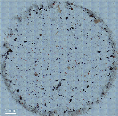 | ||
| Fig. 1 Optical overview of the sediment sample H18_21 further analysed via the manual and automated methods. | ||
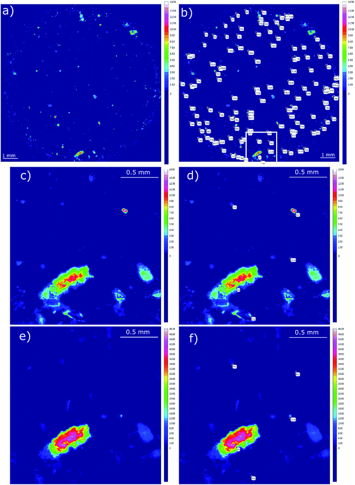
The manual analysis was started by the generation of false colour images indicating possible polymer-signatures.42 The dataset was integrated within the regions 1790–1730 cm−1 and 1480–1430 cm−1 by using OPUS© software following the methodology described by Löder et al.42 (see Fig. 2).
Afterwards the image derived from integration of the first region (1480–1430 cm−1) was divided into a grid of 4 × 4 fields with 3 mm edge length each (see Scheme 1). Manually each of these fields was magnified and all the highlighted particles were marked and consecutively numbered. Finally the spectra of marked areas (particles) were extracted by the operator and checked with a library search. In the case of improper assignments the spectra were compared and assigned by expert knowledge to reference spectra of the most common plastic polymers. In this case the spectrum was ranked by the operator. All numbered particles were listed in an Excel sheet with the matched spectra and hit quality/rank levels assigned. The same procedure was conducted for the image derived from the second region (1790–1730 cm−1) whereas solely particles that had not been marked before (first region) were selected (see Fig. 2).
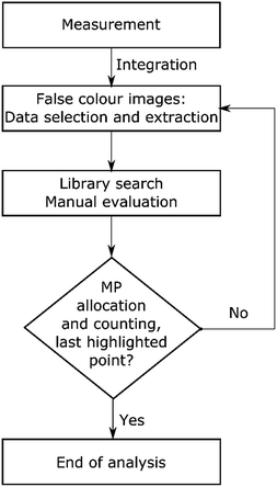 | ||
| Scheme 1 Flow chart for the procedure of transmission-FPA-FTIR data measured for full filter areas by integration of regions similar to the literature.42 | ||
The time demand for the manual analysis considering both integrated regions was 12 to 15 hours. The findings of the analysed sample are summarized in Table 1.
| Sample | PE | PP | PMMA | PS | PVC | EVOH | Sum |
|---|---|---|---|---|---|---|---|
| H18_21 | 7 | 78 | 4 | 11 | 1 | 4 | 105 |
Automated analysis by different search routines provided by the Bruker OPUS© software
The manual analysis approach encompasses several steps which are not exclusively based on software algorithms but on human recognition and decisions (expert knowledge) which increases the time demand for the analysis and the chance of misinterpretations. To overcome these restrictions the different search routines provided by the OPUS© software were combined and evaluated regarding the identification and differentiation of polymer particles. In contrast to previous studies, in which spiking with virgin plastic particles was applied,42,45,46 in our study an environmental sample was chosen for comparative analysis due to the following reasons. (1) Environmental samples contain weathered and degraded plastics.49 (2) Particles may have residues of a biofilm.50,51 Both increase the analytical demand for the automated analysis. (3) Analysis of such a sample not only provides insight into the performance of the analytical algorithm but also points to operator dependent misinterpretations induced by the intrinsic complexity of environmental samples. For spectra comparison the Bruker standard software OPUS© was used with two standard search algorithms providing scores for the degree of similarity with database entries (referred to as hit quality hereafter).The first algorithm, the so-called standard search determines the hit quality by comparison of absorption bands between measured and database spectra. An identification is true, if the position of the absorption band deviates less than the full width at half maximum (FWHM) and if the compared FWHM as well as the relative intensity deviates less than a factor of 2. For further discussion the algorithm was labelled as routine I.
The second search algorithm uses spectral correlation analysis (see eqn (1.1)) and encompasses six different routines.52
 | (1.1) |
The performance of each routine was investigated by a benchmark test. The test consisted of two major parameters, time consumption and data reliability. To perform this task several steps were included in the OPUS© macro function as depicted in Scheme 2. First the spectrum of a measured point was extracted from the 3D file and reloaded into OPUS©. The library search was performed and the result evaluated. If no hit was obtained (hit quality < 300) the extracted file was discarded. In the case of a hit the search report was saved together with the spectrum in a file labelled with the ID of the data point. Additionally the hit result with z1 for hit quality and z2 for polymer assignment was written to a text file. The ID of the spectrum was jointly derived with the x and y positions on the measurement field and stored as ID, x; y; z1; z2 within the file. The process was applied for each routine and the performance is summarized in Table 2.
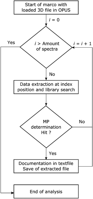 | ||
| Scheme 2 Flow chart for the automated analysis of transmission-FPA-FTIR data direct within the software via search routines provided by Bruker OPUS© using the macro function. | ||
![[thin space (1/6-em)]](https://www.rsc.org/images/entities/char_2009.gif) 192 sample spectra. I Standard routine; II vector normalization without differentiation; III vector normalization with the 1st derivative; IV vector normalization with the 2nd derivative; V MinMax normalization without differentiation; VI MinMax normalization with the 1st derivative; VII MinMax normalization with the 2nd derivative
192 sample spectra. I Standard routine; II vector normalization without differentiation; III vector normalization with the 1st derivative; IV vector normalization with the 2nd derivative; V MinMax normalization without differentiation; VI MinMax normalization with the 1st derivative; VII MinMax normalization with the 2nd derivative
| Routine | Calc. time/min | Hits | Data/GB | Time per hit/s | Time per spec./s |
|---|---|---|---|---|---|
| I | 2552 | 50![[thin space (1/6-em)]](https://www.rsc.org/images/entities/char_2009.gif) 837 837 |
0.486 | 3.02 | 0.16 |
| II | 26![[thin space (1/6-em)]](https://www.rsc.org/images/entities/char_2009.gif) 767 767 |
853![[thin space (1/6-em)]](https://www.rsc.org/images/entities/char_2009.gif) 734 734 |
8.40 | 1.88 | 1.63 |
| III | 3362 | 137![[thin space (1/6-em)]](https://www.rsc.org/images/entities/char_2009.gif) 263 263 |
1.34 | 1.47 | 0.21 |
| IV | 2320 | 73![[thin space (1/6-em)]](https://www.rsc.org/images/entities/char_2009.gif) 232 232 |
0.726 | 1.90 | 0.14 |
| V | 24![[thin space (1/6-em)]](https://www.rsc.org/images/entities/char_2009.gif) 936 936 |
873![[thin space (1/6-em)]](https://www.rsc.org/images/entities/char_2009.gif) 292 292 |
8.93 | 1.71 | 1.55 |
| VI | 20![[thin space (1/6-em)]](https://www.rsc.org/images/entities/char_2009.gif) 786 786 |
968![[thin space (1/6-em)]](https://www.rsc.org/images/entities/char_2009.gif) 192 192 |
10.0 | 1.29 | 1.29 |
| VII | >4 weeks | n.d. | n.d. | n.d. | n.d. |
In general the applied routines show that the time demand for analysis was either relatively low or high. In the first case the analysis was completed within 2300–3400 (38–57 h) minutes yielding up to 150![[thin space (1/6-em)]](https://www.rsc.org/images/entities/char_2009.gif) 000 hits. In the second case more than two weeks (above 20
000 hits. In the second case more than two weeks (above 20![[thin space (1/6-em)]](https://www.rsc.org/images/entities/char_2009.gif) 160 minutes) were necessary and hits found for the major part of the spectra. Analysis via routine VII was not complete even after four weeks calculation time and therefore stopped (data are not provided). Due to this fact, routine VII was assessed as not being suitable for the analysis pipeline. In total each analysis with MinMax normalization (V to VII) showed a high time demand as well as high hit counts. While the calculation time per hit with 1.29–1.99 s was fast, the overall time demand makes these routines unsuitable for the automated analysis. The most efficient routine regarding time demand per hit and overall time demand was routine IV.
160 minutes) were necessary and hits found for the major part of the spectra. Analysis via routine VII was not complete even after four weeks calculation time and therefore stopped (data are not provided). Due to this fact, routine VII was assessed as not being suitable for the analysis pipeline. In total each analysis with MinMax normalization (V to VII) showed a high time demand as well as high hit counts. While the calculation time per hit with 1.29–1.99 s was fast, the overall time demand makes these routines unsuitable for the automated analysis. The most efficient routine regarding time demand per hit and overall time demand was routine IV.
The major impact for the overall high demand of all calculation routines originates from the file handling of OPUS©. To prevent any loss of data, as needed for good manufacturing practices (GMPs) regulated environments,53 the data were saved directly on the hard drive during file handling and data manipulation (e.g. baseline corrections). This increases the read/write time significantly due to the lower data transfer rates compared to applications which perform the operations within random-access memory (RAM).
To determine the data quality histograms of the hit results of the different routines are depicted in Fig. S1.† The results indicate a strong dependence of the distribution towards data handling. While routine I showed a decrease in counts with hit quality, similar routines without differentiation for vector normalization (II) and MinMax normalization (V) gave a maximum of counts. If derivatives of the spectra were applied for vector normalization (III and IV) similar results compared to the standard routine (I) were achieved. The MinMax normalization (VII) was effected in a different way and the maximum shifted to a hit quality of ∼780.
To further compare the routines the quality of the database hits was determined. A manual evaluation based on expert knowledge was currently necessary for the comparison although the aim of the automated approach was to exclude human bias. The complexity of the dataset was reduced by assigning categories to matches. The major categories were derived, beginning with a correct assignment where a good resemblance was found. Uncertain assignment describes spectra which are most likely the assigned database entry but limited in their accuracy due to a bad signal to noise (S/N) ratio or the constrained complexity of the database. The third category was misassignments, where only a slight or no resemblance was found. Due to the conservative choice of categories, this approach counteracts overfitting of data by the routines. To evaluate the performance, collected data (∼550 spectra for each routine) with the highest hit quality were reopened with OPUS© (see Scheme S1†). The agreement between the assigned database spectrum and measured spectrum was evaluated. If a match without any difference was found it was marked with 1.0. For a match with one minor difference it was tagged with 0.75. Both cases were counted as certain assignments. Matches with two minor differences were assigned with 0.5 and counted as uncertain assignments. Matches with one major difference or three minor differences were marked with 0.25 or 0.01 in the case of higher values. Both cases were counted as misassignments.
This evaluation yielded confidence intervals for the use of spectra at different hit quality thresholds. It showed that in principle each routine has certain limits (see Table 3 and Fig. S2†) and exhibits obvious misassignments (even for OPUS© scores >700). In the literature, scores with a certainty above 70% (the exact output depends on the manufacturer) are described as save values.22,54 Starting with routine I a large number of misassignments and a small number of correct assignments were found. Overall, routines II and III displayed the lowest number of misassignments, but uncertain assignments were far higher compared to routine I. A similar number of uncertain assignments were accomplished by routine IV in combination with an increased number of misassignments. In comparison, routine V accomplished a greater number of correct assignments with a similar number of misassignments. In contrast, routine VI was completely unsuitable, as it yields nearly 40% misassignments. At this stage of analysis all routines displaying more than 10% misassignments were rated as unsuitable. Two routines (II and III) were further investigated. As standalone routines a large number of uncertain assignments were achieved, which limits the accuracy. The determined polymer distributions are depicted in Fig. S3 and S4.† In both cases high abundances for one type of polymer which was either cellulose (II) or acrylonitrile-butadiene-styrene (ABS) rubber (III) were found. These assignments caused the individual high uncertainty levels as they were mainly limited by the S/N ratio or a misassignment. The exact reason for this finding is still unclear. Due to the fact that both routines yielded different results when a misassignment occurred a combination of both routines was tested as an alternative to circumvent the limitation. For analysis with two routines a library search for each was introduced. Starting with routine II (see Scheme 3) the hit quality was evaluated and in the case of a positive result followed by an analysis with routine III. The spectrum was archived with a search report if the same polymer type was found by both routines. For further analysis an entry in the text file was generated containing x and y-position, the summarized hit qualities (z1) and polymer type (z2). All necessary analytical and calculating steps were introduced into a macro and handled by OPUS© with relative ease.
 | ||
| Scheme 3 Flow chart for the automated analysis of transmission-FPA-FTIR data directly via combination of search routines II and III provided by Bruker OPUS© using the macro function. | ||
The combination was found to reduce the number of overall hits to 6714 as well as the calculation time to 2830 min (47 h), which was directly correlated with the lesser number of hits. The polymer histogram and the hit quality histogram are depicted in Fig. S5.†
The previously found misassignments of cellulose by routine II and ABS by III were removed by the combination of the findings of both routines. The polymers polyethylene (PE), polypropylene (PP), polyphenylsulfone (PPSU) and two types of varnishes and the biomaterials wool and chitin yielded the major contribution of the exemplary sample. The data quality was further validated by a manual reanalysis of each polymer assignment. The confidence interval at different hit quality thresholds is depicted in Fig. S6.†
The automated analysis yielded a ratio of 82.2% correct assignments over the whole range of hit quality. Additionally, 14.7% were found to be uncertain assignments. Of the overall 6714 hits 3.1% were misassignments. In combination, 96.9% of the hits can be determined as suitable for further detailed analysis. With the macro already determining the x and y positions within the measurement field the polymer distribution could directly be converted into an image as depicted in Fig. 3.
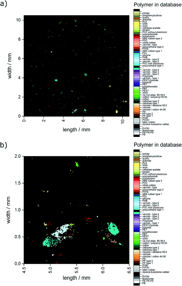 | ||
| Fig. 3 Image derived from data generated by the OPUS© Macro by the combination of two routines. (a) Complete overview over the whole filter area and (b) zoomed area similar to the area depicted in Fig. 2c–f. | ||
Image analysis of automated generated datasets
The data generated by the OPUS© macros were directly accessible to image analysis. Image analysis scripts were developed by usage of Python 3.4 with the packages numpy, matplotlib, pandas, IPython and Simple ITK.55,56First a general data processing was performed and a histogram for the pixel counts for each database entry was generated. Afterwards a grayscale overview image of the combined hit qualities was created and the dataset analysed with regard to the database assignments. To assign single pixels to particles image files were generated (additionally exported as .png) for each polymer detected. Afterwards for each image the pixels were connected by SITK Connected Component and defining an 8 pixel neighbourhood. Here each pixel was checked if it was part of a particle. If found true by the SITK function the pixel was tagged with a label assigned to a particular particle for analysis. The minimum size of a particle was set to one pixel (10.74 × 10.74 μm). After this process the number of individual labels was summed up resulting in a new dataset containing polymer specific particle sizes (as the number of connected pixels) and numbers. To access the information after analysis the dataset was stored into a .csv file.
The analysis of the data was followed by a “closing approach”. As visible in Fig. 3b, areas representing polymer particles sometimes displayed heterogeneities which could be explained by (1) differently assigned pixels (different polymers) or (2) unassigned pixels. The latter could be explained by the irregular shape of particles due to weathering processes49 or insufficiently removed biofilm50 reducing the hit quality.
In contrast to image analysis approaches, a priori defining particles as uniform (e.g. for counting bacteria) the application of imaging filters (e.g. median) was avoided to include all pixels and the referring information in the analyses.57
For particle analysis by image analysis usually images were binarized based on a certain threshold of one parameter (e.g. grey value).
However, during data evaluation (see the ESI† for details) it was found that hit quality as well as the polymer information has to be preserved for an optimal result. In this case the information of two images had to be handled simultaneously during the closing procedure as it allows the polymer specific closing and storage of hit quality for later evaluation steps. The approach had to be newly developed as no standard image analysis routine is currently available that simultaneously accesses the information of two pictures in a suitable manner.
To implement the approach into python two images based on the data of z1 for hit quality and z2 for database assignments were created. These images are data matrices (x-position, y-position, grey scale value) with the size of the maximum values of the x-position and y-position determined by the OPUS macro. During the image generation Simple ITK assigns a grey scale of 0 to all pixels which are not represented in the x, y, z1, z2 dataset. The image generated for hit quality was based on a 16-bit grey scale with values either 0 or 600–2000 if a hit was found. Similar transformation was performed for the database assignment (z2) in an 8-bit grey scale image with values from 0 to 59. For the analytical procedure it was decided to check the absence and presence of assignments via the hit quality image and the polymer assignment via the image of the database entries. The data evaluation of the needed information was introduced as one step in the script.
To target the necessary pixels in the referring script the data matrix was divided into smaller matrices. The FTIR setup always provides data with an even number of pixels as basis for the images which can be divided by the factor four. To reduce the calculation demand of the process the image was therefore parted into 4 by 4 matrices as shown below in eqn (1.2):
 | (1.2) |
Based on the matrix data, evaluation was only performed when the gap between two identified pixels was below or equal to two pixels. The two pixel gap was necessary because of the experimental setup. Each pixel represents a square on the sample with an edge length of 10.74 μm. This value was close to the wavelength-dependent diffraction limit of the IR-beam of e.g. 10 μm at 1000 cm−1. Due to the high resolution small differences on the sample surface e.g. biofilm residues influenced the spectrum generated at neighbouring pixels. Therefore the hit quality was reduced and an unassigned area in a particle can occur. Depending on the position of such deviations on the detector field two pixels can be influenced. Missed assignments can occur in each position of an 8-neighbourhood and each of these areas was targeted by analytical steps visualized in Table S1a.†
During the data evaluation the information of pixels in positions labelled with 1 was used as reference points and compared with regard to hit quality and polymer assignment. To trigger closing afterwards two requirements had to be met. First, both reference points must have a value higher than 0 in hit quality and the same database entry assigned. Secondly, all pixels marked with 0 in the rows of Table S1† (a) must be zero in hit quality. The number of necessary pixels depends on the position of the reference points with respect to each other. If they were orientated in vertical/horizontal or diagonal position to each other only the hit quality in-between has to be equal to zero. If the reference points were in a staggered position (see Table S1† case a–c) the hit quality in the direct neighbourhood facing the targeting pixels must be equal to zero as well. These requirements were necessary because such cases were mainly found in areas with a low pixel density with only a few assigned neighbours. Large and elongated assigned areas were only targeted by the horizontal/vertical and diagonal filling. Diagonal filling was found to be necessary for pixel settings representing fibres as well as to reduce artefacts from horizontal/vertical filling at corners. A similar approach as for staggered pixels was not applied and diagonal positions were evaluated after all vertical and horizontal variants had been performed.
In case all requirements are fulfilled, data are assigned to pixels between the reference points (see Table S1† row b). The value of z1 was determined as the mean value of the hit quality of the reference points. The value of z2 was set from the polymer assignment of the reference points.
During one analytical procedure each pixel was targeted once as the starting point for the matrix (position 0,0 in eqn (1.2)) to perform the process in each direction of the pixels. The whole procedure was performed with at least five iterations.
An example is shown in eqn (1.3) as input data and eqn (1.4) after successful closing.
 | (1.3) |
 | (1.4) |
In Fig. 4 the closed data are depicted. It is obvious that compared to the unmodified image (see Fig. 3) larger particles do not display unassigned areas anymore. Apparently (see Fig. 3b and 4b), the small particles were combined to larger ones by the procedure and therefore the amount of small particles was reduced.
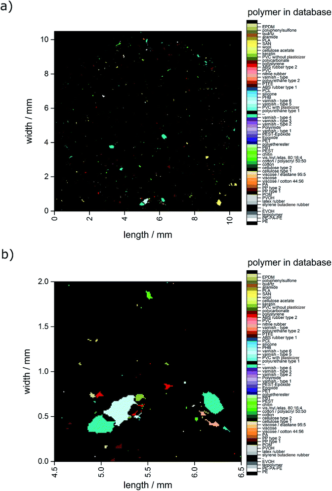 | ||
| Fig. 4 Image derived after application of the closing approach. (a) Complete overview over the whole filter area and (b) zoomed area similar to the area depicted in Fig. 2c–f. | ||
To determine the influence of the closing an image analysis was performed for these data as well. The datasets for particle distribution per database entry were further investigated. The sum of all particle counts was calculated (see Table S2†). Further, the particle size was estimated by conversion of the areas to metric numbers. The particle size was multiplied with the edge length of a single pixel (10.74 μm) on the grid. To facilitate comparisons of data the particles were binned into different size classes. For assignment to size-bins the particles were treated as square areas. The index values in the figures and tables shown below represent the edge length of one square side. In Fig. 5 the direct comparison for the analysis of the data before and after closing is depicted. The number of single pixels and small particles was reduced significantly by closing and the number of small particles below a size of 25 μm was reduced by 35%. Above 25 μm the trend was reversed and more particles were found. The number of particles was reduced from 1530 particles before to 1097 after the closing approach.
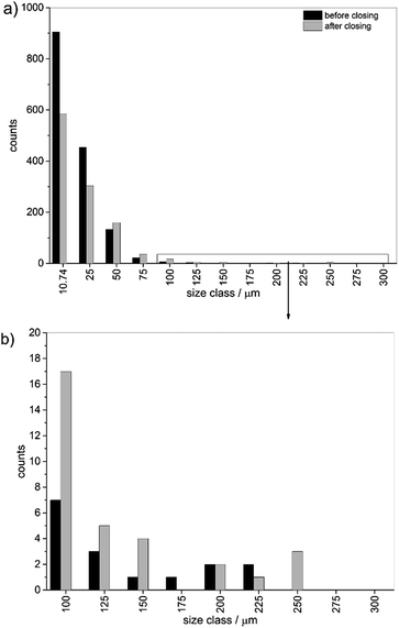 | ||
| Fig. 5 Overall particle size distribution binned into size classes before and after closing (a) full distribution and (b) zoom into particle bins for classes higher than 75 μm. | ||
Comparison between manual and automated analyses
For the sediment sample considered as an example, in total 733 polymer particles were found by the herein presented automated analysis pipeline (see Fig. 6 and Table S2†), which is almost seven fold higher compared to the manual analysis (see Fig. 6). In addition, further types of polymers were identified, mainly different copolymers (terpolymer, ethylene-propylene-diene (EPDM) and polyester-epoxide (PEST-EP)), varnish and rubber (ABS, styrene-acrylonitrile resin (SAN)) as well as other polymers (polycarbonate (PC), polyoxymethylene (POM), PPSU) and polyvinyl alcohol (PVOH). For most of the previously manually identified polymers higher abundances were found. In particular PE, PP and polyvinyl chloride (PVC) were clearly underestimated by manual analysis due to the fact that mainly small particles were missed. However during automated analysis no assignments were found for poly(methyl methacrylate) (PMMA), yet several types of varnishes are based on acrylates and might contain these particles. For ethylene vinyl alcohol (EVOH) no assignments were found by automated analysis but a similar abundance of PVOH particles was observed. The chosen sample storage and purification (PVC bottle and PC filter material) would have influenced the results for PC (1 particle) and PVC (33 particles), yet the grade of possible contamination became apparent only after automated analysis. Therefore the use of a different storage container (if applicable) and filter material as well as running of procedural blanks is advised.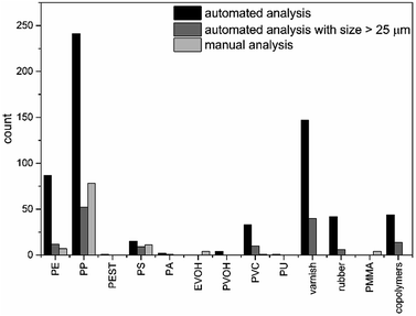 | ||
| Fig. 6 Comparison of 12 polymer classes found by automated analysis for all size classes (black), starting from particles larger than 625 μm2 (dark grey) and derived via manual analysis (light grey). | ||
The different findings of automated versus manual analysis in terms of numbers and identities can be explained as follows. Firstly, although false colour images based on integrals provide a fast overview to estimate possible MP particles, the application of integrals42 has a major drawback at lower S/N ratios and complex samples. The standard integration method uses a baseline between the upper and lower wavenumbers of the chosen area for integration. If the S/N ratio was low, these bands had low integral values caused by the noise in the spectrum. The same can be found for complex samples where influences from e.g. background material can artificially lower the integral value. In both cases the particle might be overlooked in false colour images. In the case of the automated analysis each spectrum was compared with the database and all points uniformly evaluated. In this case an assignment was found even if compared to the manual analysis the integral value in the false colour image was low.
Further, automated and image analysis assigned large areas similar to the ones in false colour images (see Fig. 2c and e and 4b). In the manual analysis the area was tagged and counted as one particle. In contrast, the automated analysis yielded a mixture of different particles which were all in close neighbourhood. A higher number of particles were counted because by the automated library search differences have a higher influence on the overall dataset than by the point based manual analysis. The operator often could only perform a library search for up to five points on such a particle due to the high time demand of the overall analysis.
In addition, false colour images are often dominated by high values of a few types of polymers. Smaller particles and particles with a lower absorbance in the specific regions were overlooked with relative ease, because they were simply not visible under these circumstances. About 52% of the automated identified particles were of the smallest size class which was also only barely visible in false colour images.
As previously shown, small particles were nearly completely overlooked during manual analysis. To facilitate comparison between the analyses, particles below 25 μm were excluded for further discussion. Under these circumstances 163 particles (see Fig. 6 and Table S2†) were found, which is still 1.5 times higher than the manual results. For PE and polystyrene (PS) a similar amount of particles were found. The value for PP was clearly under-represented and a lower abundance found compared to the manual analysis. Still high abundances of PVC, varnish and copolymers were present. This indicates that by manual analysis mainly particles with a size down to 30 μm can be detected which is in agreement with the literature,42,44 while complex signal settings were harder to detect.
However the time consumption for the automated analysis was found to be rather high yet the process can be parallelized by executing the macros and scripts on several computers. To reduce the calculation time further optimizations are underway.
Conclusions
The herein presented spectroscopic analysis pipeline is a novel analytic routine to provide reliable data on the identity, number and size of MPs in environmental samples enriched on filter membranes. Compared to manually derived data, possibly biased decisions based on expert knowledge are only necessary in very few steps. While the analytical time demand was found to be still high, the process can be parallelized by usage of multiple low performance but rather inexpensive office computers. Single identification routines proved to be limited in accuracy while the combination of two routines yielded error values below 3% for an autonomous database search. The data processing is able to handle files containing up to one million spectra. The generated data could be transferred to images allowing a polymer specific analysis regarding the number and size of particles. By polymer specific closing of areas it was demonstrated that this approach is highly recommended for particle analysis. The reduction of personal demand based on our approach allows monitoring of MPs down to small size classes with relative ease and high comparability. Our results clearly indicate that MPs < 30 μm exist in the natural environment. However, a lower size limit cannot be specified due to the diffraction limit and the applied method.Acknowledgements
This work was supported by the German Federal Ministry of Education and Research (Project BASEMAN – Defining the baselines and standards for microplastics analyses in European waters; BMBF grant 03F0734A). The authors thank the crew of the RV Heincke for technical support. S. P. thanks Dr Gernot Höhne (Bruker Optics GmbH, Ettlingen) for the help during macro development. C. L. thanks the Deutsche Bundesstiftung Umwelt (DBU) for financial support.Notes and references
- PlasticsEurope, Plastics – the Facts 2015, accessed 20.01.2016, 2016.
- D. K. A. Barnes, F. Galgani, R. C. Thompson and M. Barlaz, Philos. Trans. R. Soc., B, 2009, 364, 1985–1998 CrossRef CAS PubMed.
- J. Hopewell, R. Dvorak and E. Kosior, Philos. Trans. R. Soc., B, 2009, 364, 2115–2126 CrossRef CAS PubMed.
- J. R. Jambeck, R. Geyer, C. Wilcox, T. R. Siegler, M. Perryman, A. Andrady, R. Narayan and K. L. Law, Science, 2015, 347, 768–771 CrossRef CAS PubMed.
- A. Lechner and D. Ramler, Environ. Pollut., 2015, 200, 159–160 CrossRef CAS PubMed.
- T. Mani, A. Hauk, U. Walter and P. Burkhardt-Holm, Sci. Rep., 2015, 5, 17988 CrossRef CAS PubMed.
- S. Zhao, L. Zhu and D. Li, Environ. Pollut., 2015, 206, 597–604 CrossRef CAS PubMed.
- C. Wilcox, G. Heathcote, J. Goldberg, R. Gunn, D. Peel and B. D. Hardesty, Conservat. Biol., 2015, 29, 198–206 CrossRef PubMed.
- R. P. Vieira, I. P. Raposo, P. Sobral, J. M. S. Goncalves, K. L. C. Bell and M. R. Cunha, J. Sea Res., 2015, 100, 91–98 CrossRef.
- M. Bergmann, L. Gutow and M. Klages, Marine Anthropogenic Litter, Springer, Cham, Heidelberg, New York, Dordrecht, London, 2015 Search PubMed.
- R. C. Thompson, C. J. Moore, F. S. vom Saal and S. H. Swan, Philos. Trans. R. Soc., B, 2009, 364, 2153–2166 CrossRef CAS PubMed.
- M. Cole, P. Lindeque, E. Fileman, C. Halsband, R. Goodhead, J. Moger and T. S. Galloway, Environ. Sci. Technol., 2013, 47, 6646–6655 CrossRef CAS PubMed.
- N. von Moos, P. Burkhardt-Holm and A. Koehler, Environ. Sci. Technol., 2012, 46, 11327–11335 CrossRef CAS PubMed.
- O. Setala, V. Fleming-Lehtinen and M. Lehtiniemi, Environ. Pollut., 2014, 185, 77–83 CrossRef CAS PubMed.
- D. Brennecke, E. C. Ferreira, T. M. M. Costa, D. Appel, B. A. P. da Gama and M. Lenz, Mar. Pollut. Bull., 2015, 96, 491–495 CrossRef CAS PubMed.
- A. J. R. Watts, C. Lewis, R. M. Goodhead, S. J. Beckett, J. Moger, C. R. Tyler and T. S. Galloway, Environ. Sci. Technol., 2014, 48, 8823–8830 CrossRef CAS PubMed.
- E. Besseling, E. M. Foekema, J. A. Van Franeker, M. F. Leopold, S. Kuhn, E. L. B. Rebolledo, E. Hesse, L. Mielke, J. Ijzer, P. Kamminga and A. A. Koelmans, Mar. Pollut. Bull., 2015, 95, 248–252 CrossRef CAS PubMed.
- O. M. Lonnstedt and P. Eklov, Science, 2016, 352, 1213–1216 CrossRef PubMed.
- P. Farrell and K. Nelson, Environ. Pollut., 2013, 177, 1–3 CrossRef CAS PubMed.
- L. Gutow, A. Eckerlebe, L. Gimenez and R. Saborowski, Environ. Sci. Technol., 2016, 50, 915–923 CrossRef CAS PubMed.
- L. M. Ziccardi, A. Edgington, K. Hentz, K. J. Kulacki and S. K. Driscoll, Environ. Toxicol. Chem., 2016, 35, 1667–1676 CrossRef CAS PubMed.
- R. C. Thompson, Y. Olsen, R. P. Mitchell, A. Davis, S. J. Rowland, A. W. G. John, D. McGonigle and A. E. Russell, Science, 2004, 304, 838 CrossRef CAS PubMed.
- K. L. Law and R. C. Thompson, Science, 2014, 345, 144–145 CrossRef CAS PubMed.
- M. Burke, Chem. Ind., 2011, 9 Search PubMed.
- GESAMP, GESAMP, Rep. Stud., 2015, 90, 1–98 Search PubMed.
- I. Hintersteiner, M. Himmelsbach and W. W. Buchberger, Anal. Bioanal. Chem., 2015, 407, 1253–1259 CrossRef CAS PubMed.
- A. Hoffman and K. Turner, J. Chem. Educ., 2015, 92, 742–746 CrossRef CAS.
- C. Hogue, Chem. Eng. News, 2014, 92, 36–37 Search PubMed.
- C. Hogue, Chem. Eng. News, 2013, 91, 23–25 Search PubMed.
- H. K. Webb, J. Arnott, R. J. Crawford and E. P. Ivanova, Polymers, 2013, 5, 1–18 CrossRef.
- T. M. Davidson, Mar. Pollut. Bull., 2012, 64, 1821–1828 CrossRef CAS PubMed.
- P. L. Corcoran, M. C. Biesinger and M. Grifi, Mar. Pollut. Bull., 2009, 58, 80–84 CrossRef CAS PubMed.
- V. Hidalgo-Ruz, L. Gutow, R. C. Thompson and M. Thiel, Environ. Sci. Technol., 2012, 46, 3060–3075 CrossRef CAS PubMed.
- F. Galgani, G. Hanke, S. Werner, L. Oosterbaan, P. Nilsson, D. Fleet, S. Kinsey, R. C. Thompson, J. v. Franeker, T. Vlachogianni, M. Scoullos, J. M. Veiga, A. Palatinus, M. Matiddi, T. Maes, S. Korpinen, A. Budziak, H. Leslie, J. Gago and G. Liebezeit, Guidance on Monitoring of Marine Litter in European Seas, 2013 Search PubMed.
- G. Liebezeit and F. Dubaish, Bull. Environ. Contam. Toxicol., 2012, 89, 213–217 CrossRef CAS PubMed.
- J. A. Ivar do Sul, M. F. Costa and G. Fillmann, Water, Air, Soil Pollut., 2014, 225, 2004 CrossRef.
- Y. K. Song, S. H. Hong, M. Jang, G. M. Han, M. Rani, J. Lee and W. J. Shim, Mar. Pollut. Bull., 2015, 93, 202–209 CrossRef CAS PubMed.
- M. G. J. Löder and G. Gerdts, in Marine Anthropogenic Litter, ed. M. Bergmann, L. Gutow and M. Klages, Springer International Publishing, 2015, ch. 8, pp. 201–227, DOI:10.1007/978-3-319-16510-3_8.
- E. Fries, J. H. Dekiff, J. Willmeyer, M.-T. Nuelle, M. Ebert and D. Remy, Environ. Sci.: Processes Impacts, 2013, 15, 1949–1956 CAS.
- E. Dümichen, A.-K. Barthel, U. Braun, C. G. Bannick, K. Brand, M. Jekel and R. Senz, Water Res., 2015, 85, 451–457 CrossRef PubMed.
- D. Fischer, A. Kaeppler and K.-J. Eichhorn, Am. Lab., 2015, 47, 32–34 Search PubMed.
- M. G. J. Löder, M. Kuczera, S. Mintenig, C. Lorenz and G. Gerdts, Environ. Chem., 2015, 12, 563–581 CrossRef.
- J. P. Harrison, J. J. Ojeda and M. E. Romero-Gonzalez, Sci. Total Environ., 2012, 416, 455–463 CrossRef CAS PubMed.
- A. Käppler, D. Fischer, S. Oberbeckmann, G. Schernewski, M. Labrenz, K.-J. Eichhorn and B. Voit, Anal. Bioanal. Chem., 2016, 408, 8377–8391 CrossRef PubMed.
- A. S. Tagg, M. Sapp, J. P. Harrison and J. J. Ojeda, Anal. Chem., 2015, 87, 6032–6040 CrossRef CAS PubMed.
- A. Kaeppler, F. Windrich, M. G. J. Loeder, M. Malanin, D. Fischer, M. Labrenz, K.-J. Eichhorn and B. Voit, Anal. Bioanal. Chem., 2015, 407, 6791–6801 CrossRef CAS PubMed.
- H. K. Imhof, J. Schmid, R. Niessner, N. P. Ivleva and C. Laforsch, Limnol. Oceanogr.: Methods, 2012, 10, 524–537 CrossRef CAS.
- M. G. J. Löder, H. K. Imhof, M. Ladehoff, C. Lorenz, S. Mintening, S. Primpke, S. Piehl, I. Schrank, C. Laforsch and G. Gerdts, manuscript in preparation.
- A. L. Andrady, in Marine Anthropogenic Litter, ed. M. Bergmann, L. Gutow and M. Klages, Springer International Publishing, 2015, ch. 3, pp. 57–72, DOI:10.1007/978-3-319-16510-3_3.
- J. P. Harrison, M. Schratzberger, M. Sapp and A. M. Osborn, BMC Microbiol., 2014, 14, 232–246 CrossRef PubMed.
- S. Dobretsov, in Biofouling, Wiley-Blackwell, 2010, pp. 123–136, DOI:10.1002/9781444315462.ch9.
- Bruker, OPUS/IR Reference Manual, Bruker Optik GmbH, Ettlingen, 2014 Search PubMed.
- European Commission, Official Journal of the European Union, 2013, C 343/01, 1–14 DOI:10.3000/1977091X.C_2013.343.eng.
- R. W. Obbard, S. Sadri, Y. Q. Wong, A. A. Khitun, I. Baker and R. C. Thompson, Earth's Future, 2014, 2, 315–320 CrossRef.
- B. C. Lowekamp, D. T. Chen, L. Ibanez and D. Blezek, Frontiers in Neuroinformatics, 2013, 7, 45, DOI:10.3389/fninf.2013.00045.
- T. S. Yoo, M. J. Ackerman, W. E. Lorensen, W. Schroeder, V. Chalana, S. Aylward, D. Metaxas and R. Whitaker, in Medicine Meets Virtual Reality 02/10, ed. J. D. Westwood, H. M. Hoffman, R. A. Robb and D. Stredney, IOS Press, Amsterdam, 2002, pp. 586–592 Search PubMed.
- M. Sonka, V. Hlavac and R. Boyle, Image Processing, Analysis, and Machine Vision, Cengage LearningUnited States of America, 4th edn, 2015 Search PubMed.
Footnote |
| † Electronic supplementary information (ESI) available. See DOI: 10.1039/c6ay02476a |
| This journal is © The Royal Society of Chemistry 2017 |

