Machine learning-assisted materials development and device management in batteries and supercapacitors: performance comparison and challenges

Abstract

Machine learning (ML) has been the focus in recent studies aiming to improve battery and supercapacitor technology. Its application in materials research has demonstrated promising results for accelerating the discovery of energy materials. Additionally, battery management systems incorporating data-driven techniques are expected to provide accurate state estimation and improve the useful lifetime of batteries. This review briefs the ML process, common algorithms, advantages, disadvantages, and limitations of first-principles materials science research techniques. The focus of discussion is on the latest approaches, algorithms, and model accuracies for screening materials, determining structure–property relationships, optimizing electrochemical performance, and monitoring electrochemical device health. We emphasize the current challenges of ML-based energy materials research, including limited data availability, sparse datasets, and high dimensionality, which can lead to low generalizability and overfitting. An analysis of ML models is performed to identify the most robust algorithms and important input features in specific applications for batteries and supercapacitors. The accuracy of various algorithms for predicting remaining useful life, cycle life, state of charge, state of health, and capacitance has been collected. Given the wide range of methods for developing ML models, this manuscript provides an overview of the most robust models developed to date and a starting point for future researchers at the intersection of ML and energy materials. Finally, an outlook on areas of high-impact research in ML-based energy storage is provided.

---

1. Introduction

Electrochemical energy storage has become central to everyday life and is critical for transitioning society to renewable energy sources. Improvements to these energy storage systems are urgently needed for enhancing their energy density, power density, safety, cost, and lifetime. Many research studies have focused on the computational discovery of novel energy materials.¹ Significant advances in computing power and methods based on density functional theory (DFT) have enabled researchers to simulate and calculate the properties of complex atomic systems with high accuracy.² This led to high-throughput screening of candidate materials, but in a restricted search space, making materials discovery for electrochemical energy storage difficult and time-consuming.³ The rise of data-driven machine learning (ML) has opened up the possibility to search much wider material spaces with both high speed and accuracy.⁴

1.1 Machine learning overview

Machine Learning involves the use of algorithms that can be used to identify the underlying hidden patterns and relationships within a dataset. It has been used to perform seemingly simple human tasks from speech recognition,⁵ image recognition,⁶ and driving,⁷ to highly complex tasks like time series forecasting,⁸ cancer diagnoses,⁹ and anomaly detection.¹⁰ ML has been very influential in various fields with the growing amount of data being collected and transmitted everywhere. Its success in many of these applications has allowed ML to become central to everyday life.

ML algorithms can be placed into four main categories: supervised, unsupervised, reinforced, and semi-supervised learning.¹¹ Supervised learning algorithms utilize labeled data, where the model determines the relationship between known features and an output. Meanwhile, unsupervised learning algorithms are utilized when the data has no labels. This allows users to identify hidden patterns and gain insights from a large, complex dataset that has no ground truth. Semi-supervised learning algorithms are the middle ground between supervised and unsupervised learning, where the available data has both labeled and unlabeled observations. Reinforcement learning also does not use ground truth labels but is capable of taking actions that maximize rewards to ultimately reach a solution.¹² These algorithms provide flexible and efficient approaches to discovering new understandings from “big data”. The decision tree in Fig. 1 illustrates the situations in which each type of ML algorithm can be used.

Fig. 1 Decision tree identifying when supervised, semi-supervised, unsupervised, and reinforcement learning should be used.

Most approaches in physical science studies rely on supervised learning algorithms to train models that make predictions.¹³ In prediction tasks, each data point is described by a set of features or descriptors, and the output ground-truth label of a data point is already known. A trained supervised ML model uses this set of features to map the relationship to its respective output label. Prediction tasks that involve supervised ML include regression and classification, where the output is a continuous value and a categorical label, respectively. A key element of supervised learning is that error can be evaluated quantitatively based on discrepancies between the prediction and the actual output, also known as a loss function. During training, an optimization algorithm like gradient descent is used to minimize this loss function and achieve the minimum error.

Although less commonly used in physical science studies, unsupervised learning algorithms are important for descriptive tasks, like clustering and anomaly detection.¹⁴ As with supervised ML, each data point is described by a set of features. However, the output label of a data point is unknown, and rather than predicting a continuous value as the output, the output is the cluster or clusters that a data point belongs. The purpose of unsupervised ML is to enable the automatic labeling of data points in a dataset, which would be extremely time-consuming to manually perform. The challenge of unsupervised learning tasks is that without any ground-truth labels, determining model performance is much more difficult. Evaluating unsupervised models requires internal validation metrics, which rely on quantifying how similar data points within the same cluster are to each other and how different they are from data points in other clusters.

Semi-supervised learning is especially useful in physical science studies, where small labeled datasets are commonly an issue. One important application is active learning, where the algorithm is initially trained on a labeled dataset and then poses queries to the user in a human-in-the-loop process to determine the label for the queried data point.¹⁵ This framework has excellent potential in accelerating the search for optimal material designs through guided experimentation, as will be demonstrated throughout this review.

Reinforcement learning is different from both supervised and unsupervised learning in that no initial dataset is needed. The concept is inspired by behavioral psychology, where the algorithm learns through trial and error, ultimately aiming to maximize a reward function while interacting with its environment.¹⁶ It also has great potential for accelerating the materials design processes.

1.2 Common algorithms

ML can be applied and utilized using a wide variety of interfaces, such as scikit-learn,¹⁷ Tensorflow,¹⁸ Pytorch,¹⁹ Keras,²⁰ Armadillo,²¹ and several others. On top of this, there is a wide variety of algorithms that can be utilized, with some of the most prominent mentioned here.

1.2.1. Linear regression. Linear regression falls under the supervised classification of ML algorithms. It consists of two main types which are simple regression and multivariable regression. Simple regression relates a single feature to a single output value in the form of eqn (1).²²

Y = βx + C + ε (1)

where C is the y-intercept, β is the coefficient, x is the value of the feature, and ε is noise. Multiple features can also be accounted for using multiple regression shown in eqn (2).

Y = β₁x₁ + β₂x₂ +…+ β_nx_n +C +ε (2)

Linear regression is attractive due to its excellent interpretability, unparalleled performance when dealing with linear data, as well as its simplicity. For example, Fig. 2a shows how the data points would be modeled by linear regression, where increasing x values lead to increasing y values. On the other hand, dealing with linear regression introduces some disadvantages that include the assumption of linearity between input and output variables, as well as being insufficient in modeling complex relationships.²³ However, nonlinearity may be accounted for by using the “kernel trick”, which transforms a feature before performing the regression.²²

Fig. 2 Representations of (a) linear regression, (b) logistic regression, (c) decision tree, and (d) support vector machine.

1.2.2. Logistic regression. The logistic regression algorithm can be described as a linear regression model that is passed through a sigmoid function, allowing the model to be applied to classification problems, where the output is a probability between 0 and 1. The form of the logistic regression equation follows eqn (2), which is then constrained through the sigmoid function in eqn. (3).²⁴

The classification with the highest probability is the output. This is demonstrated in Fig. 2b, where data points lie between two categories (binary classification) based on the independent variable. Logistic regression is resilient to overfitting, has high computational efficiency, avoids making assumptions regarding the distribution of classes, and achieves high accuracy with linear problems. However, logistic regression is prone to overfitting and is unable to accurately model nonlinear decision boundaries.²⁵

1.2.3. Decision tree. The decision tree (DT) is a supervised ML algorithm that generates a tree consisting of nodes, leaves, and branches, and can perform classification and regression tasks.²⁵ It works through the progressive splitting of nodes based on different parameters to reach the leaves that represent the output. As shown in Fig. 2c, DT can output continuous values for regression tasks with the ability to model nonlinear functions. DTs have great interpretability, require minimal data preparation, perform well with a nonlinear correlation between the parameters, and have the ability to identify feature importance.²⁶ However, it is prone to overfitting and is not able to make predictions for data outside the range of the training set.²⁷

1.2.4. Support vector machine. Support vector machine (SVM) is a supervised ML algorithm based on the structural risk minimization principle that is well suited for classification and regression. In regression tasks, SVM uses a kernel function to transform the data to a higher dimension. Fig. 2d demonstrates the hyperplane that is drawn with surrounding boundary lines that form the margin of tolerance. This algorithm has gained noticeable popularity due to its competency in dealing with homogenous data.²⁸ SVMs have demonstrated excellent generalization capabilities and have good performance with linearly constrained quadratic problems.²⁹ Choosing the optimal kernel function has a strong influence on accuracy and can be difficult to tune, and SVM may not perform well with large datasets.³⁰

1.2.5. Artificial neural network. The artificial neural network (ANN), inspired by the biological neural network, is a collection of connected parameterized functions.³¹ Similar to a biological brain, ANN operates by receiving a set of inputs, processing the signal through layers of neurons, and outputting a transformed signal. At each neuron, all the neurons from the previous layer are multiplied by a weight and are summed together to get a value, which is then passed through an activation function. Through consecutive epochs, optimal weight distribution for each neuron connection is attained through backpropagation. ANN can generate both linear and non-linear models, thereby introducing a broader range of applications in comparison to other algorithms.³² ANNs are also reputable for generating outputs despite the corruption of some neurons, having a distributed memory, parallel processing capability, and an ability to generalize to unseen data.³³

1.3 Advantages of ML

ML has been utilized in the energy storage sector due to its capability of drastically increasing computational speed, comprehending complex mechanisms, and optimizing performance through energy storage management systems.³⁴ A successful ML model performs predictions that are cheap and accurate, allowing researchers to identify materials with desirable properties without the need for costly experiments or simulations.³⁵ In physics-based ML, complicated physical processes are modeled solely through learned relationships between the input and output values of a given dataset.³⁶ These methods are currently used for finding new materials through crystal structure prediction, which can greatly reduce the consumption of DFT calculation and computing resources, and composition prediction.³⁷ ML algorithms are easily able to learn high-dimensional data, where hundreds of different features can be utilized as input. Algorithms such as deep neural networks and support vector regression (SVR) can be trained to accurately predict values of highly dynamic systems, such as state of charge (SOC) in electric vehicles, where constantly changing external factors and driving behaviors play a significant role.^38,39 However, there also exists a tradeoff between the accuracy of the ML model compared to DFT.⁴⁰ Currently, ML enables rapid predictions for high-throughput tasks, but at a lower accuracy, while DFT allows for high accuracy at the expense of speed and high computational cost. The most prominent advantage of ML is that as more data is continuously collected and published through experimentation, training datasets will also expand, therefore, increasing the size of potential training datasets for ML models to continue becoming more accurate and generalizable.

1.4 Disadvantages of ML

Though ML has many useful applications for researchers, there are still several disadvantages that need to be discussed. According to the “No Free Lunch” theorem, all ML algorithms will have the same average performance for all possible optimization problems.⁴¹ Thus, it is important to test a variety of algorithms and identify which performs best for a particular problem. With each approach, different levels of accuracy can be achieved with varying levels of efficiency.^38,39,42,43 Several ML algorithms also require hyperparameter tuning, an important step for choosing the best model configuration to achieve the highest accuracy. This can become time-consuming in some cases, such as with neural networks, where several possible hyperparameters can be selected, leading to very expensive training if all possible configurations were to be tested. Bayesian optimization (BO), Particle Swarm Optimization, genetic algorithms (GAs), and several other methods have been employed to improve hyperparameter optimization.⁴⁴ In addition, feature engineering can drastically increase the number of ML training runs needed to identify the best subset of features. Proper feature selection is necessary as it can have significant implications on model accuracy, generalizability, and complexity.⁴⁵ Since algorithms strictly learn from a provided dataset during training, bias present in any dataset must be considered when making predictions, as an insufficient amount of data can cause model accuracy and generalizability to suffer.⁴⁶ Datasets must be homogenized and processed before they can be used, taking into account the input shape and format supported by the algorithm. Careful attention must be taken to prevent training unnecessarily complex models, which can cause overfitting to a specific dataset and limit practicality.⁴⁷ Overfitting is a common issue, especially with small, high-dimensional datasets, but can be mitigated through feature elimination. The advantages and disadvantages of the entire ML process are summarized in Fig. 3.

Fig. 3 Advantages and disadvantages of machine learning. Created with http://biorender.com/.

1.5 Combining ML with first-principles approaches

DFT and molecular dynamics (MD) are widely used first-principles techniques for simulating atomic structures and computing the properties of materials through approximations of the laws of quantum mechanics.⁴⁸ The only inputs that are required to carry out calculations are crystal structure and material composition. Theoretical first-principles simulations have been widely used for elucidating structure–property relationships, probing rational synthesis methodologies, and providing invaluable experimental guidance.⁴⁹ Despite having greater cost efficiency than conventional trial-and-error experimentation and providing theoretical guidance, first-principles methods have limits. They require solving the many-particle Schrödinger equation, which currently requires several approximations. Consequently, its accuracy is limited in various situations that are yet to be resolved.⁵⁰ There is also a limited ability to simulate complex experimental conditions due to high computational requirements, with denser and more complex structures being particularly more computationally expensive.⁵¹ The high computational cost of first-principles modeling also makes it an inefficient high-throughput technique for screening vast amounts of materials or discovering new materials.⁵² DFT is limited to calculations ranging from several tens to a few thousand atoms, as its complexity increases cubically with the number of atoms.⁵³ And with MD being computationally intensive, simulations are very time-restricted, lasting from tens to hundreds of picoseconds.⁵⁴ An application of an active learning algorithm is shown in Fig. 4a, where on-the-fly ML was used to minimize the cost of training an interatomic potential model used in MD simulations of Li-ion diffusion. This method increased the efficiency of MD by 7 orders of magnitude and calculates migration energies in close agreement with experimental values.

Fig. 4 (a) Active learning coupled with MD to simulate the collective diffusion of Li-ions in Li₃B₇O₁₂, where colored arrows illustrate simultaneous movement direction. Reprinted with permission from ref. ⁵⁴. Copyright 2020 American Chemical Society. (b) General workflow for developing machine learning models and their application in energy materials research. Some applications of trained machine learning models include guided experimentation and data mining. Created with http://biorender.com/.

By combining ML algorithms with first-principles computations, the result is a trained model that can quickly derive material properties. This allows researchers to screen for candidate materials from large materials databases and predict properties of novel materials without having to perform any more time-consuming computational simulations.^40,55–57 A general workflow for developing ML models and their application in materials science research is illustrated in Fig. 4b. Researchers that have applied ML methods to DFT calculations discovered that optimized models were capable of making accurate predictions of material properties outside of the training dataset.⁵⁸ Some researchers have even bypassed performing DFT calculations by using easily accessible material properties from previous experiments or materials databases to make predictions for other properties, reducing the computational cost of the materials screening process by several orders of magnitude.^59,60 A hierarchy demonstrating materials design through a combination of ML, first-principles methods, and experimentation is illustrated in Fig. 5. At the bottom is experimentation, the slowest among the methods, which provides the ground truth information. In the next layer up is computational simulation like DFT and MD, which is faster than experimentation, but still computationally inefficient and constrained in its abilities. At the top is ML with the highest speed for properties prediction, but can have limited accuracy and generalizability. Data from experiments and computational simulations are leveraged for training and improving models that map features to target properties in ML models. For materials discovery and design through ML, the ultimate goal is to accelerate the identification of new materials with excellent properties outside of the given training dataset. Thus, model extrapolation is necessary, followed by verification through theoretical simulations and experimentation.

Fig. 5 Hierarchy of materials design through ML involving a framework of experimentation, computational simulations, and ML model training. Adapted from ref. ¹¹⁸, ^196–198 with permission from Elsevier and the Royal Society of Chemistry. Copyright 2018 Elsevier. Copyright 2018 Royal Society of Chemistry. Created with http://biorender.com/.

Determining structure–function relationships from training datasets through ML is key to significantly accelerating materials discovery and design.⁶¹ ML was first developed around the 1950s. Some techniques commonly used in ML, such as linear and logistic regression, were introduced much earlier, as shown in the timeline of Fig. 6a. In the general ML workflow, the first step involves data collection. This can be done through experimentation or first-principles calculations or can be collected from public databases. Next, pre-processing data includes splitting the dataset into training and test sets, normalization, and homogenization. Then, feature engineering can be carried out to reduce dimensionality, remove highly correlated features, decrease model complexity, and improve model accuracy.⁶² Working with high-dimensional data can lead to sparse and computationally intensive models. Some commonly used dimensionality reduction techniques include principal component analysis (PCA), Pearson correlation, and least absolute shrinkage and selection operator (LASSO). During model training, techniques such as grid search and cross-validation are used for hyperparameter optimization. Evaluation metrics, commonly including coefficient of determination (R²), root mean squared error (RMSE), mean absolute error (MAE), and mean absolute percent error (MAPE) are then used to quantify model accuracy.⁶³ Ultimately, ML can be used to generate knowledge-based rules for screening a large number of materials.⁶⁴ Another application of ML is active learning systems capable of guiding experimentation to achieve much faster material design and optimization.⁶⁵ ML has also been introduced for estimating the health of energy storage devices like batteries and supercapacitors with computational efficiency useful for real-time management.³⁴ As shown in Fig. 6b and c, the number of publications regarding the application of ML in battery and supercapacitor research each year in the past decade has grown substantially.

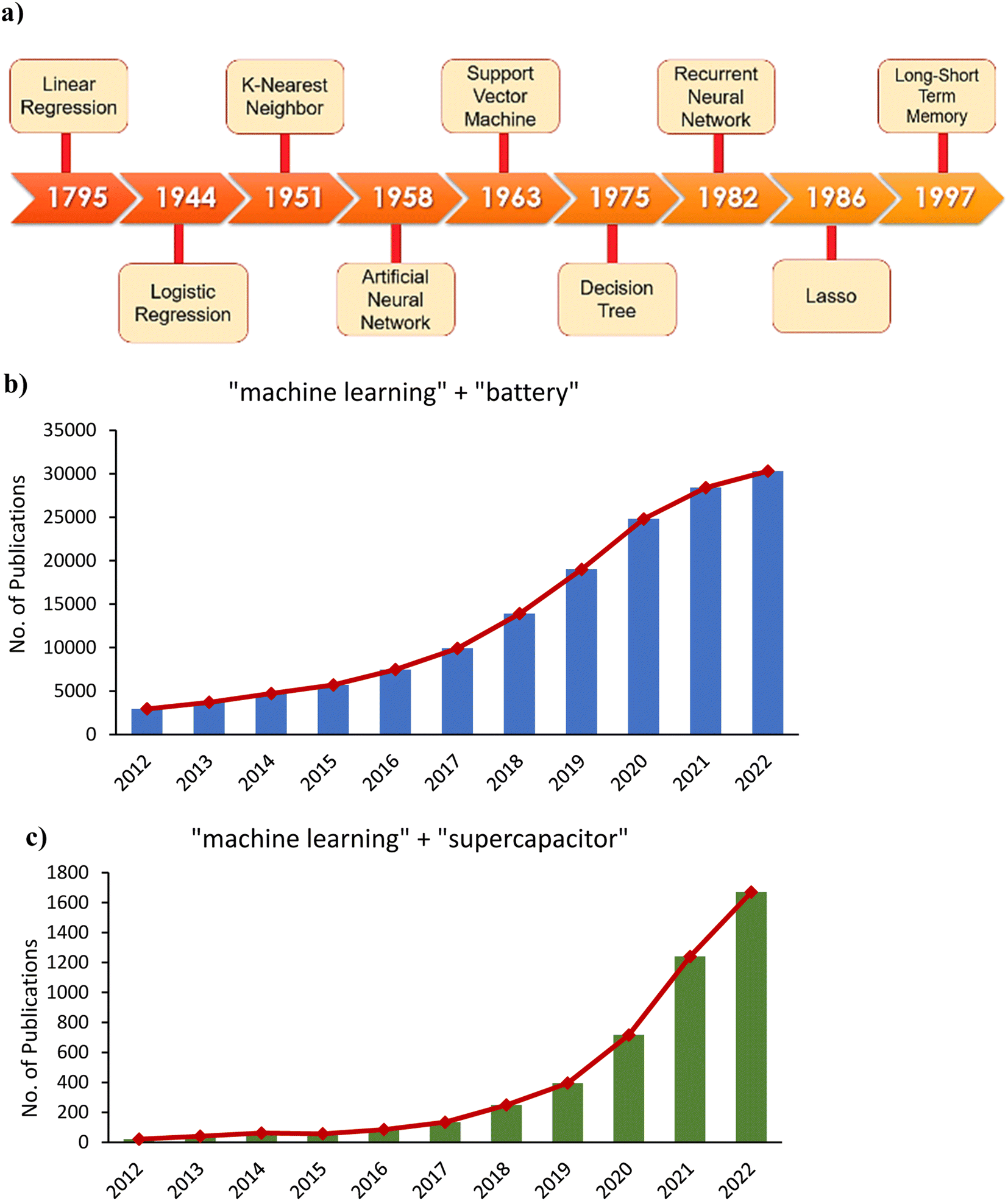Fig. 6 (a) Timeline depicting the introduction of various ML algorithms. The number of publications in 2012–2022 on (b) machine learning and batteries, and (c) machine learning and supercapacitors. Data obtained from Google scholar (https://scholar.google.com/)

ML has demonstrated high-quality results for designing energy storage materials that have been experimentally validated by researchers in a design-to-device process. The design-to-device process is key for confirming the accuracy of ML and simulated optimal materials design. Liow et al. demonstrated a design-to-device approach by training a gradient boosting regression (GBR) model to predict the discharge capacities of Li-ion batteries (LIBs) based on cathode synthesis variables.⁶⁶ Experimental validation of the optimal synthesis parameters demonstrated a high discharge capacity of 209.5 mA h g⁻¹ and coulombic efficiency of 86%. Similarly, for a supercapacitor design-to-device approach, Ghosh et al. used a RF model to predict the specific capacitance of a novel electrode material, cerium oxynitride, and observed a RMSE of 0.3 F g⁻¹.⁶⁷ With experimental validation, the synthesized supercapacitor achieved a high specific capacitance of 214 F g⁻¹ and high cyclic stability of 100% after ∼10 000 cycles. Park et al. employed a combined ML-DFT screening using a multilayer perceptron (MLP) model to screen formation energies of layered-oxide K-ion battery cathode materials.⁶⁸ After screening potential candidates, the predicted material with the greatest stability was K_0.3Mn_0.9Cu_0.1O₂, which was then synthesized to experimentally validate the simulated data. The synthesized compound proved to be in good agreement with the predicted values, with the synthesized battery demonstrating high discharge capacity, power density, and cyclic stability. Dave et al.¹⁴⁵ proposed a closed-loop experimental process that combines robotics for automated experimentation with a Bayesian optimization framework to optimize the ionic conductivity of non-aqueous electrolytes. After 42 experimental iterations, 6 electrolytes were measured with ionic conductivities above 12 mS cm⁻¹. When applied in a cell for validation, the proposed electrolyte demonstrated improved discharging capacity after 4C fast-charging. Overall, this achievement demonstrated a 6-fold time acceleration compared to random search experimentation. Verduzco et al. demonstrated the effectiveness of ML in accelerating the search for high ionic conductivity lithium lanthanum zirconium oxide (LLZO) garnets.⁶⁹ Emulating the search for the highest ionic conductivity LLZO garnet as of 2020, the researchers utilized an active learning framework to guide which experimental data points to train the RF model on and predict the best candidate composition. Ultimately, 30% fewer experimental investigations of different LLZO garnets published since 2005 were necessary to identify the highest ionic conductivity composition. As described above, ML has already demonstrated its potential for accelerating the search for novel high-performing energy storage materials through studies that have carried out the entire design-to-device process.

Previous reviews on ML-guided energy materials and energy storage devices research have demonstrated a trend of novel approaches allowing for an expanding number of more complex applications. Chen et al. provided a critical review of the applications of ML to predict ionic conductivity, elastic moduli, and interatomic potentials of Li compounds.⁷⁰ Wang et al. focused on recent applications of ML for predicting the electrochemical performance of carbon-based supercapacitors.⁷¹ Liu et al. compiled several studies regarding the application of ML to predict the properties of rechargeable battery electrolytes and electrode materials.⁷² Kang et al. portrayed how ML applications for energy materials have assisted quantum chemistry techniques, allowing for the prediction of electronic structure, crystal structure, LIB performance, and the optimization of experimental studies.⁷³ These reviews are mainly focused on the novel applications of ML research in energy materials and storage devices, but there is a need for a review of the predictive accuracy of these approaches to highlight the most promising approaches and the most robust models for specific applications.

This review compares and provides insights into the accuracies of recently developed ML approaches in energy materials research. Here, we provide a review of recently developed ML-guided models applied to predicting energy material properties, discovering materials, and predicting and optimizing the performance of batteries and supercapacitors. We also provide a direct comparison of the various ML algorithms that have been proposed to clearly illustrate their prediction accuracies, highlight the most successful models, and recommend future directions for ML studies in energy storage technology. Finally, we highlight opportunities for future research in applying ML to aid advancements in energy materials.

2. Predicting material properties

The ability to understand complex, nonlinear structure–property relationships is crucial for accelerating the discovery of high-performance energy storage materials.^74,75 To uncover these structure–property relationships, data from experiments and first-principles calculations must be collected. Many researchers have utilized published material datasets, such as the Materials Project,⁷⁶ Open Quantum Materials Database (OQMD),⁷⁷ Automatic FLOW for Materials Discovery (AFLOW),⁷⁸ Novel Materials Discovery (NOMAD),⁷⁹ and several others. By significantly reducing the computational costs of first-principles calculations for screening large datasets of candidate materials, ML can accelerate the discovery of new high-performance energy storage materials.

2.1 Redox potential

Redox potential characterizes a material's tendency to be reduced or oxidized, a crucial property for identifying high voltage and high energy density electrode materials.⁸⁰ When considering candidate electrode materials, predicting the redox potential through DFT modeling is computationally expensive.⁸¹ Organic cathode materials have become extensively researched due to their environmental friendliness, low cost, and tunable electronic nature.⁸² Allam et al. developed ANN, GBR, and kernel ridge regression (KRR) models to predict the redox potential of carbon-based electrode materials.⁵⁸ The researchers utilized LASSO and Pearson correlation to reduce the number of features from 20 875 to 7. KRR achieved the lowest training RMSE of 0.158 V, and when applied to materials outside the range of the training data, the model had a 3.94% MAPE, demonstrating excellent generalizability. Doan et al. trained a Gaussian process regression (GPR) model to predict oxidation potentials of homobenzylic ether (HBE) redoxomers.⁵⁷ With a training set of 1400 HBEs and 49 structural features, PCA reduced the number of features to 15, allowing GPR to achieve a test set RMSE of 0.097 V. The first two principal components are illustrated in Fig. 7, where most of the variance is explained and the molecules are larger towards the right. Furthermore, they were able to incorporate an active learning BO process with a GPR surrogate model to efficiently select desirable redoxomers from an unseen dataset of 112 000 HBEs, starting with 10 randomly selected for training. By fitting a probabilistic model to a dataset, BO can utilize the model uncertainty to guide where to evaluate the function next to find the global optimum in the fewest number of steps.⁸³ The BO process utilized expected improvement (EI) for selecting the next best candidate. EI is an acquisition function that balances between generalizing from current best estimates (exploitation) and searching through regions of higher uncertainty (exploration).⁸⁴ This helps prevent converging at local optimums and expedites the search for target properties. The researchers observed a 5-fold improvement in optimal HBE screening efficiency using the BO approach compared to random selection. Fig. 8a demonstrates the efficient training process through the BO approach in comparison to ground truth DFT values.

Fig. 7 2D representation of homobenzylic ether molecules by reducing 49 features into 2 principal components, and color-coded by oxidation potential. Reprinted with permission from ref. 57. Copyright 2020 American Chemical Society.

Fig. 8 (a) GPR prediction of optimal oxidation potentials (1.40–1.70 V) guided by Bayesian optimization, allowing for a 5-fold increase in efficiency over DFT. Reprinted with permission from ref. 57. Copyright 2020 American Chemical Society.⁸⁵ (b) Examples of designed features based on the number of atoms with the same coordination number, rings, and radicals. Reprinted with permission from ref. 85. Copyright 2018 American Chemical Society.⁹⁰

The redox stability of electrolytes is also essential for ensuring electrochemical stability at the anode and cathode. Okamoto & Kubo applied Gaussian KRR and GBR to predict the redox potentials of electrolyte additives for LIBs using a dataset of 149 entries.⁸⁵ The researchers developed a method for describing the molecular structures using a total of 22 structural features. The features, shown in Fig. 8b, describe the number of atoms with the same coordination number, the number of rings, and indicate any radicals. GBR demonstrated the highest accuracy for predicting both reduction and oxidation potentials, achieving R² scores of 0.851 and 0.643 in the test set, respectively. In contrast to the two previous studies mentioned, performing feature elimination led to slightly lower accuracy. In the test set, model accuracy suffered due to the presence of outliers. Under closer examination, the outliers predicted by ML helped to reveal the possible underestimation of reduction potentials by the ab initio molecular orbital calculations used for ground truth values. This interesting find illustrates how ML can reveal patterns in the dataset that otherwise would have gone unnoticed.

Radical redox-active polymers have gained attention recently as a cleaner and low-cost alternative to metal-based materials in batteries.⁸⁶ This has attracted the attention of ML researchers looking to quickly predict the properties of polymeric materials and avoid the high computational cost of atomistic simulations. Li & Tabor trained a GPR model using electron affinity estimated through the semi-empirical GFN2-xTB method, molecular fingerprints, and 3D descriptors, a relatively simple set of input features, to predict the reduction potential of polymers.⁸⁷ The cross-validation results achieved an R² of 0.83 when compared to experimental values, demonstrating the strong potential for this method to lower the computational cost of DFT calculations by coupling GPR with a semi-empirical method.

With a small dataset, low generalizability and low predictive accuracy are difficult to overcome, even with feature elimination. From these studies, some of the most important features identified include electron affinity, HOMO–LUMO gap, number of tricoordinate carbons, number of tetracoordinate carbons, number of monodentate oxygen atoms, and number of bidentate oxygen atoms. Table 1 summarizes the ML models mentioned here trained for redox potential prediction. Among the studies mentioned here, it is unclear whether KRR or GBR has better performance for redox potential prediction. However, GPR has gained attention for this specific application, achieving an RMSE below 0.01 V due to its nonparametric form, making it useful for more complex mapping functions.⁵⁷ GPR is widely used among computational chemists and material scientists due to its ability to interpolate between high dimensional data points and its probabilistic nature that enables uncertainty quantification.⁸⁸ Through uncertainty quantification, ML can be utilized to expedite high-throughput screening and accelerate the discovery of materials with extraordinary properties in an active learning process.

Table 1 Summary of ML models used for redox potential prediction

Machine learning algorithm	Advantages	Disadvantages	Performance	Ref.
ANN	Effective non-linear modeling, good generalizability, implicit feature selection	Requires extensive hyperparameter tuning, prone to overfitting, error increases with feature elimination	RMSE = 0.179 V	58
KRR	Fits non-linear data well, relatively simple	Strong reliance on kernel selection, unstable with multicollinearity, requires composite features	RMSE = 0.158 V	58
			R ^2 = 0.801 (reduction potential)	85
			R ^2 = 0.512 (oxidation potential)	85
GBR	Effective non-linear modeling, implicitly selects features	Large number of hyperparameters, requires a large training dataset	RMSE = 0.212 V	58
			R ^2 = 0.851 (reduction potential)	85
			R ^2 = 0.643 (oxidation potential)	85
GPR	High accuracy, provides uncertainty quantification	Poor efficiency with large datasets	RMSE = 0.097 V	57
			RMSE = 0.28 V (reduction potential)	87

---

2.2 Crystal structure

Predicting the crystal structure of compounds is an important issue and a priority for materials science research as it governs many physical and chemical properties. Being able to quickly and easily predict the likely crystal structure of a molecule will help researchers better understand how crystal structure is correlated with different material properties.⁵⁶ In an approach to training an ML model capable of predicting crystal structure, Graser et al. constructed a random forest (RF) model trained with a database of 24 215 formulae.⁵⁵ A high accuracy ranging between 97% to 85% was achieved. When predicting class type, average recall decreased from 73% to 54% as more classes were added because many classes had only one or two data points. This result illustrates the deterioration of ML models trained with sparse data, a common challenge faced by material science researchers with limited data availability. In another approach, Cheng et al. developed a graph network (GN) to predict DFT-based formation energies from atomic and structural features and then performed BO to identify the optimal crystal structure.⁸⁹ The researchers' method maps a crystal graph to its formation energy. Therefore, predicting crystal structure entails optimizing a crystal graph to achieve minimum formation energy. With a dataset of 320 000 structures, the GN achieved a test set MAE of 26.9 meV per atom using 50% for training data and 50 meV per atom using 25% for training data. In the BO process, Cheng et al. began with 200 random crystal structures and were able to successfully predict the ground-state rock salt structure in 5000 steps.⁸⁹ Though a perfect crystal structure prediction has not yet been achieved by GNs, this BO framework provides a highly efficient method that avoids performing a prohibitive number of expensive DFT calculations. A later study by Cheng et al. substantiates the potential for a GN approach paired with BO for crystal structure prediction. With a dataset of 132 000 compounds and 50% used for training, an MAE of 20.8 meV per atom was achieved, or a 22.7% improvement over their previous model.⁹⁰ This can be attributed to the two additional features including crystal symmetry and occupancy of the Wyckoff position that was implemented for generating the crystal structures. Although the accuracy of this ML approach may not be at the level of DFT calculations, its computation efficiency is three orders of magnitude greater, as shown in Fig. 9. In an active learning approach using moment tensor potentials, Podryabinkin et al. predicted the low-energy structures of carbon, sodium, and boron allotropes.⁵³ Their ML-based interatomic potential model could accurately predict the low energy structures for carbon, sodium, and boron structures using up to 5 orders of magnitude fewer DFT calculations compared to the number of evaluated configurations.

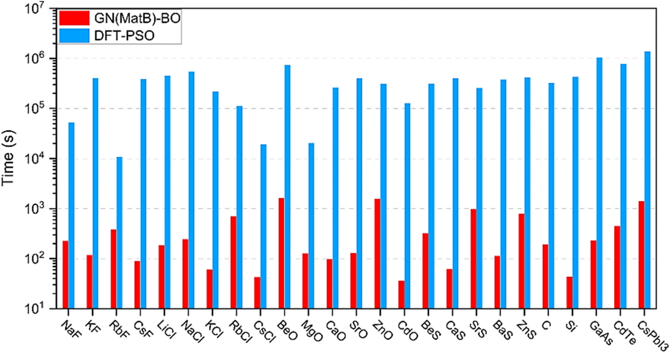Fig. 9 Time comparison of GN paired with Bayesian optimization (GN-BO) to DFT paired with particle swarm optimization (DFT-PSO) for prediction of 25 different crystal structures. GN-BO requires three orders of magnitude less time compared to DFT-PSO. Reprinted with permission from ref. ⁹⁰. Copyright 2022 Springer Nature.

Current research in crystal structure prediction has shown the prevalence of active learning frameworks, specifically BO, and the importance of uncertainty quantification. This approach can drastically decrease computational cost by a few orders of magnitude compared to DFT. However, it is still a challenge for researchers to identify an ML model with high prediction accuracy for predicting crystal structures. Table 2 summarizes the performance of the ML models in the studies mentioned here. GNs show good potential as they can easily represent the structural features as crystal graphs, but this area of research still needs more attention.

Table 2 Summary of ML models used for crystal structure prediction

Machine learning algorithm	Advantages	Disadvantages	Performance	Ref.
RF	High accuracy, not prone to overfitting, provides feature importance, implicitly selects features	Computationally intensive with larger datasets and more trees	Accuracy = 85–97%	55
SVM	Self-adjusts kernel function, scales up to high-dimensional data well	Strong reliance on kernel selection	Accuracy = 87–93%	55
GN	Enables physically meaningful descriptors for crystal structure	Currently low accuracy	MAE = 20.8 meV per atom	89

---

2.3 Dielectric breakdown

Dielectric materials are the building blocks of dielectric capacitors, which are used in many ultrahigh power-density applications.⁹¹ Dielectrics can store electrostatic energy by polarization under an external electric field.⁹² However, as advancements are made to miniaturize electronic devices, the dielectric breakdown strength significantly decreases due to the lower thermal and mechanical stability of a smaller dielectric.^93,94 Additionally, current dielectric materials suffer from low energy densities.⁹⁵ The dielectric breakdown mechanism relies on complex chemical, electrical, thermal, and mechanical interactions that are not fully understood.⁹⁶ A framework for calculating dielectric breakdown strength has been established through DFT calculations, but this is a highly time-consuming method.⁹⁷

Shen et al. performed least squares regression (LSR) to predict the dielectric breakdown of polymer-based nanocomposites as a function of dielectric constant, electrical conductivity, and Young's Modulus, obtaining an R² value of 0.91 for the training/test set combined.⁹⁶ The predictive function generated by LSR demonstrated that adding nanofillers with low dielectric constant and low electrical conductivity to the polymer nanocomposite improves dielectric breakdown strength. Kim et al. utilized KRR, RF, and LASSO to predict the intrinsic dielectric breakdown field of dielectrical insulators with a dataset of 82 entries.⁹³ Though all three models achieved similar predictive accuracies, only LASSO generated an explicit functional formula, which related band gap and maximum phonon frequency to the dielectric breakdown field, achieving a test set R² of 0.72. Their LASSO model revealed that boron-containing compounds were most consistently identified as having a high dielectric breakdown. Using the same dataset as Kim et al., Yuan et al. used genetic programming to search for the best function for predicting dielectric breakdown, also finding that band gap and maximum phonon frequency were the most important features.⁹⁷ Their best model had a lower RMSE of 237 MV m⁻¹ compared to 692 MV m⁻¹ using the LASSO model determined by Kim et al. The genetic programming method was able to improve upon prediction accuracy, while also balancing speed and accuracy. However, in both approaches, overfitting to training data was a common risk. Kumar et al. proposed an approach that addresses the issue of instability and overfitting of ML models to small datasets.⁵⁹ Using the same dataset of materials and 8 features used by Kim et al., Bootstrapped projected gradient descent was used to select the most important features along with dimensional analysis through the Buckingham-Pi Theorem. The researchers arrived at an equation relating band gap and nearest-neighbor distance to the intrinsic breakdown field, achieving an R² of 0.85, outperforming the LASSO model obtained by Kim et al.

Currently, low data availability on dielectric breakdown has significantly affected the accuracy of trained ML models. The most common ML pipeline for predicting dielectric breakdown involves using a nonlinear function to generate compound features. Band gap, nearest neighbor distance, and phonon cutoff frequency have been found to have high importance in dielectric breakdown prediction. Table 3 summarizes the performance of the ML models used in the studies mentioned here. Future studies should continue exploring more ML algorithms and investigate how to overcome the issue of low predictive accuracy and limited generalizability when training on small datasets.

Table 3 Summary of ML models used for dielectric breakdown prediction

Machine learning algorithm	Advantages	Disadvantages	Performance	Ref.
LSR	High accuracy, simple and efficient, outputs mathematical function relating descriptors to target	Strong sensitivity to outliers, requires iterative optimization and good starting parameter values	R ^2 = 0.91	96
KRR	Performs well with high dimensionality, calculates feature importance	Strong reliance on kernel selection	R ^2 = 0.69	93
RF	Calculates feature importance, performs well with high dimensionality	Computationally intensive with larger datasets and more trees, low accuracy	R ^2 = 0.64	93
LASSO	Performs feature selection, outputs mathematical function relating descriptors to target	Unstable with multicollinearity, requires composite features	R ^2 = 0.72	93
Genetic programming	Outputs mathematical function relating descriptors to target, automatically generates composite descriptors	Prone to overfitting, may converge at local minimum	RMSE = 1.48 MV m^−1	97

---

2.4 Band gap

Band gap values are important for the classification of compounds as metals, semiconductors, or insulators for applications in electronic energy storage and conversion devices.^98,99 It is an essential parameter for determining electronic conductivity. A narrow band gap (high electronic conductivity) is generally needed in electrode materials, while a wide band gap (low electronic conductivity) is needed for solid electrolytes.¹⁰⁰ However, the high computational demand and time requirement needed to perform complex band gap calculations prevents DFT-based methods from being practical for characterizing large amounts of materials. In one study by Zhuo et al., SVM, k-nearest neighbors (KNN), KRR, and logistic regression were trained to identify nonmetals from inorganic solids in a dataset of 4916 experimentally determined band gaps.¹⁰¹ With SVM achieving the highest accuracy, the area under the receiver operating characteristic (ROC) curve was 0.97, comparable to the accuracy of DFT. Then, SVR was used for predicting the band gap values of the nonmetals, which attained a test set RMSE of 0.45 eV. When applied to compounds outside the database, SVR attained an RMSE of 1.46 eV, an improvement over a DFT-based model with an RMSE of 2.1 eV. The accuracy of this approach demonstrates that ML can significantly lower the computation requirements of predicting band gaps compared to DFT-based calculations, while simultaneously being more accurate. The researchers observed that SVR underestimated high band gap values, which was attributed to the lack of data for high band gap materials. An approach utilized by Rajan et al. was a GPR model trained to predict band gap values of MXenes.¹⁰² LASSO reduced the features from 47 to 8, and then KRR, SVR, GPR, and bootstrap aggregating (bagging) methods were used to predict GW-calculated band gaps from a training set of 76 MXenes. With GPR performing the best, an R² of 0.83 and an RMSE of 0.14 eV were achieved in the test set. The training set utilized by Rajan et al. was restricted to MXenes with band gaps around 1.5 to 3.5 eV, allowing for a much lower RMSE compared to the wide-ranging band gaps of around 0.06 to 10 eV in the training set utilized by Zhuo et al. Clearly, restricting the training set of a model can prove beneficial for enhancing the predictive accuracy of the model, though at the expense of generalizability.

Materials databases are commonly insufficient in size and diversity for training highly accurate ML models, resulting in underfitting. Zhang et al. found that increasing model accuracy is associated with increasing degrees of freedom (and data size), as demonstrated in Fig. 10a.¹⁰³ This higher degree of freedom leads to lower accuracy in unknown domains. By incorporating a crude estimation property, or a low accuracy prediction of the target property through non-expensive Generalized Gradient Approximation (GGA) calculations, the researchers decreased the RMSE of a KRR model by 33% (0.34 eV) in band gap prediction. This demonstrates a feasible approach for increasing the accuracy of models with high bias, when collecting more data is too expensive or not an option.

Fig. 10 (a) KRR cross-validation RMSE achieved for prediction of band gaps as a function of the average degree of freedom and data size of the training set. Reprinted with permission from ref. 103. Copyright 2018 Springer Nature. (b) Convex hull of Li–Ge calculated through DFT and predicted using SVR and KRR models. Reprinted with permission from ref. 105. Copyright 2019 Elsevier.

Among recent studies on band gap prediction, SVR, GPR, and KRR are the most commonly used. Table 4 summarizes these studies and compares their performances. GPR was demonstrated to have very low prediction error out of these algorithms. As mentioned in a few studies, the lack of data on wide band gap materials has limited the accuracy and generalizability of ML. A potential workaround is to limit the dataset to materials with more narrow band gaps at the expense of generalizability. Another proposal is the use of a crude estimation property that can improve model accuracy with inexpensive computations. Further studies should be performed on overcoming low data availability in band gap prediction.

Table 4 Summary of ML models used for band gap prediction

Machine learning algorithm	Advantages	Disadvantages	Performance	Ref.
SVM	High accuracy, excellent generalizability	Strong reliance on kernel selection	RMSE = 0.45 eV	101
			RMSE = 0.17 eV	102
KNN	Simple to implement, nonparametric modeling	Poor efficiency with larger dataset, challenging optimization of number of neighbors, sensitive to outliers	RMSE = 0.54 eV	101
KRR	Relatively simple	Low accuracy, strong reliance on kernel selection	RMSE = 0.72 eV	101
			RMSE = 0.19 eV	102
GPR	High accuracy, highly efficient, improves with more features	Poor efficiency with larger datasets	RMSE = 0.14 eV	102
Bootstrap aggregating	Not prone to overfitting, calculates feature importance	Low interpretability	RMSE = 0.16 eV	102
LASSO	Outputs mathematical function relating descriptors to target	Unstable with multicollinearity	RMSE = 0.71 eV	103

---

2.5 Formation energy

The stability of a material depends on fundamental thermodynamic properties, such as formation energy, that rely on computationally intensive DFT calculations to determine.¹⁰⁴ The major challenge for developing ML models capable of predicting formation energies is in representing crystal structure data and interatomic interactions in a suitable input format.¹⁰⁵ Faber et al. utilized KRR and varying molecular Coulomb matrix representations of molecules to predict formation energy, training with a dataset of 3938 crystal structures.¹⁰⁶ The researchers found that model accuracy increased with increasing training data size, with their most accurate method of representation achieving a test set MAE of 0.37 eV per atom. Krajewski et al. optimized an ANN model to predict the formation energies of structures by utilizing 271 features, including elemental and crystal structural attributes derived from Voronoi tessellations.¹⁰⁴ Their model achieved a test set MAE of 30 meV per atom after removing less-stable structures with formation energies above 250 meV per atom, and an MAE of 41 meV per atom when applied to a subset of more complex structures. This demonstrated the increased predictive accuracy and generalizability achieved by ML models by restricting the chemical space of the dataset. Honrao et al. utilized KRR and SVR to predict both unrelaxed and relaxed formation energies using a DFT-calculated dataset of 14 168 Li–Ge crystal structures.¹⁰⁵ The researchers represented crystal structure data through partial radial basis functions. The test set RMSE of the KRR model was 20.4 meV per atom and 20.3 meV per atom for unrelaxed and relaxed energies, respectively, while SVR was 20.8 meV per atom and 20.9 meV per atom, respectively.

Noh et al. proposed an approach that applies uncertainty quantification to crystal graph convolutional neural networks (CNNs) through Monte Carlo sampling and dropout for formation energy prediction.¹⁰⁷ In each iteration, interlayer connections between neurons are randomly dropped with a 0.2 probability, and 200 random samples are taken to produce a Bayesian approximation. The Monte Carlo sampling mean and variance correspond with the formation energy prediction and uncertainty, respectively. The materials that pass the formation energy screening criteria within a 95% confidence interval undergo detailed DFT relaxations to refine the prediction of the most promising material candidates. With this scheme and a dataset consisting of >7000 materials, 67% of the materials selected by a direct DFT screening method were successfully identified, while also reducing the required number of DFT calculations by a factor >50. Without uncertainty quantification, only 39% of the materials were successfully identified. This study demonstrates the significant performance boost to high-throughput screening offered by uncertainty quantification of ML models. Further exploration of this uncertainty quantification approach should be applied to other material properties and algorithms in high-throughput screening applications.

Overall, KRR and ANN have both demonstrated good accuracy levels for formation energy prediction, even achieving high accuracy in predicting the convex hull of Li–Ge shown in Fig. 10b. Table 5 summarizes the ML models mentioned here for predicting formation energies. Further studies should continue exploring how crystal structure information can be represented in input formats understandable by ML models. Other algorithms, such as graph neural networks should be further explored for formation energy prediction, as their accuracy is currently low.

Table 5 Summary of ML models used for formation energy prediction

Machine learning algorithm	Advantages	Disadvantages	Performance	Ref.
KRR	Relatively simple, fits non-linear data well	Strong reliance on kernel selection, does not scale to larger datasets well	RMSE = 20.3 meV per atom	105
SVR	Efficient with large datasets	Strong reliance on kernel selection	RMSE = 20.9 meV per atom	105
ANN	Dropout reduces model size with little impact on accuracy, excellent generalizability, capable of transfer learning	Requires extensive hyperparameter tuning, prone to overfitting	RMSE = 66.1 meV per atom	104

---

3. Applications for batteries

Growing efforts toward electrification have accelerated the demand for batteries. LIBs specifically have gained widespread use in applications including portable electronics and electric vehicles. However, further enhancements are still required in battery technology to satisfy future needs in automotive applications, including improvements to energy density, cycle life, cost, safety, fast charging, and more sustainable materials.¹⁰⁸ Accelerating demand for batteries will require aggressive production ramp-up and an increase in raw material supplies. Growing consideration over unsustainable materials and fragile supply chains has directed many research efforts toward eliminating these critical elements.^109,110

3.1 Designing and optimizing electrodes

In the search for novel electrode materials, there is a need for computationally efficient models to aid in the understanding of how composition, pore structure, morphology, ionic conductivity, and charge storage influence each other to design high-performing batteries and supercapacitors.^111–114 Besides materials development, many studies have also explored rational design of these novel electrode materials to enable scalable energy storage material synthesis.¹¹⁵ Trial and error experimentation has provided a majority of current efficient LIB electrode materials,¹¹⁶ and DFT calculations have exposed important rules for designing electrodes.¹¹⁷ However, the high computational expense of DFT methods for modeling large systems would be unreasonable for a vast number of materials.^118,119 This motivates researchers to develop highly efficient ML tools capable of providing fast and accurate performance predictions for electrode materials.

Research on “beyond Li-ion” technologies like Na, K, Ca, Mg, and Al-ion batteries has been gaining attention recently with their potential to achieve lower costs and greater energy density.¹²⁰ Joshi et al. trained deep neural network, SVR, and KRR models for the prediction of the voltage range with a training set of 3977 electrode materials consisting of Li-ion and several alternative metal ion compounds.¹²¹ PCA reduced the feature vector dimensionality from around 237 to 80, allowing all three ML methods to achieve test set MAE of 0.42–0.46 V. Surprisingly, when the models were used to predict Na electrode voltage ranges, MAE improved from 0.93–1.25 V when using the entire training dataset to 0.62–0.70 V when using Li materials only. Though Na materials were not contained in either of these datasets, the dataset containing only Li materials was more coherent than the dataset containing 6 different materials that were comprised of 65% Li materials. This demonstrates the importance of having a coherent training set, and the detriment that can be caused by including sparse material data. However, this may be an issue that can be overcome through the use of transfer learning to predict properties of the sparser materials.

Houchins et al. trained a Behler-Parrinello neural network model for predicting energy–volume curves, entropy, and Gibbs energy of NMC cathodes with a dataset of 12 962 points, performing in good agreement with DFT calculations and experimental measurements.¹¹⁷ Then, using grand canonical Monte Carlo simulations to simulate Li-vacancy ordering or discharging/charging of the cathode, the neural network was able to accurately predict the voltage profiles of the NMC cathode and several other cathode materials. Okubo et al. investigated how well RF can predict the improvement of cathode capacity retention based on coating, doping, electrolyte additives, functional binders, cut-off voltage, and C-rate.¹²² The test set achieved only R² of 0.52, likely a result of the limited dataset size. Most notably, the C-rate and cut-off voltage were identified as having the largest influence on capacity retention improvement. Takagishi et al. developed an ANN regression model for predicting the specific resistance of Li-ion electrode structures, which performed with an R² of 0.99 on validation data.¹²³ Then, BO was applied to solve the inverse problem of optimizing the process parameters for manufacturing a battery electrode with the minimum specific resistance, which was predicted to be 47 Ω m. This framework is demonstrated in Fig. 11.

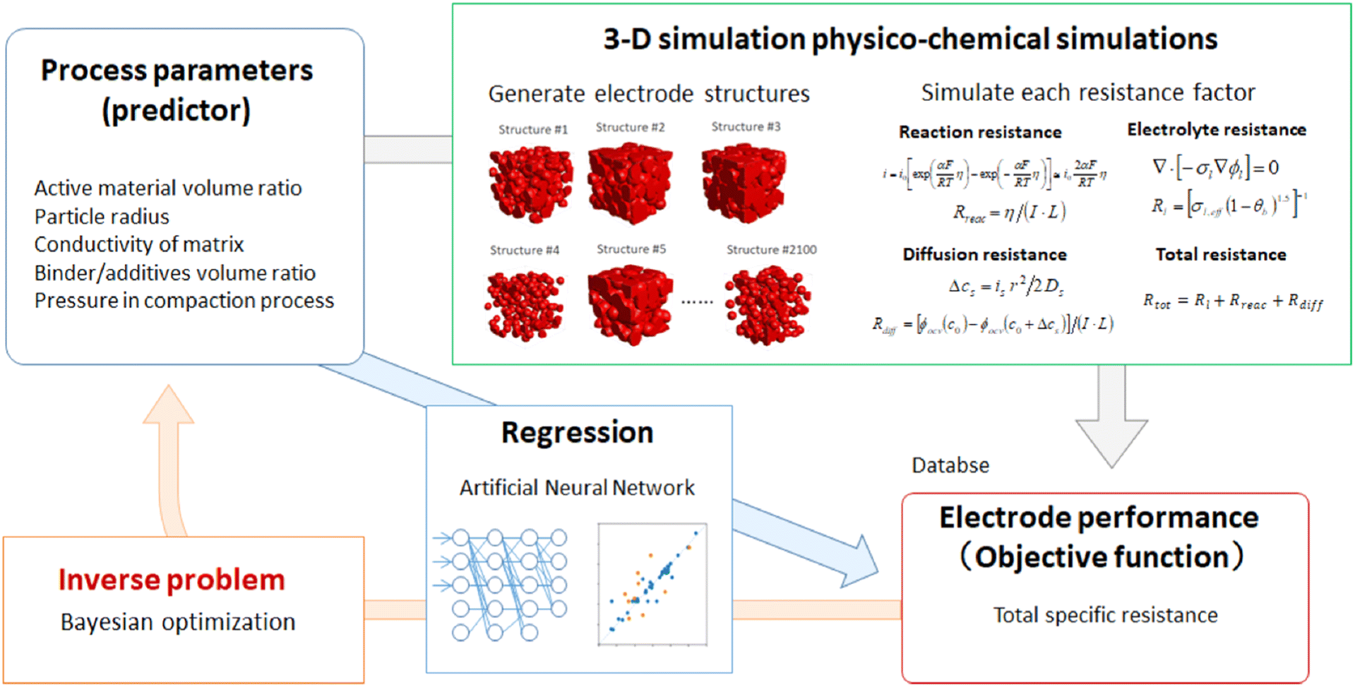Fig. 11 Workflow for predicting Li-ion battery electrode specific resistance by utilizing 3D physio-chemical simulations and an ANN model. Further, Bayesian optimization was performed to identify the optimal electrode properties and processing parameters. Reprinted with permission from ref. ¹²³. Copyright 2019 Multidisciplinary Digital Publishing Institute.

Data from both successful and failed experiments can be leveraged by ML to assist synthetic chemists in determining optimal synthesis conditions. Moosavi et al. developed an approach based on the combination of experimentation, ML, and GA to determine the optimal conditions for synthesizing metal organic frameworks (MOFs) by varying 9 parameters, ultimately achieving a BET surface area of 2045 m² g⁻¹.¹²⁴ The idea behind this approach is to use GAs to guide the selection of the 9 experimental parameters while analyzing crystallinity and phase purity as the objective function. After collecting data from over 120 failed and partly successful experiments, the researchers trained a RF model on the 9 parameters to predict crystallinity and phase purity. From this trained RF model, the importance of each parameter was obtained and used as a quantified form of chemical intuition to search the chemical space more effectively in subsequent experiments. In other words, by varying the most important parameters as determined by RF much more frequently than the least important ones, the chemical space can be explored more efficiently without sacrificing sampling accuracy, significantly increasing the probability of successful synthesis conditions. This study demonstrates the importance of utilizing both failed and successful experiments in training ML models to obtain strong chemical intuition and accuracy for searching chemical spaces much more efficiently. However, researchers and journals typically do not publish failed experimental data, wasting valuable information that could be used in training less biased and more useful ML models.

Quantum mechanical approaches aided by data-driven ML have been proposed to discover structure–property relationships in electrode materials. Deringer et al. utilized Gaussian approximation potential (GAP) trained with DFT data to predict the energies of porous and graphitic carbon systems, with accuracy within 2 kJ mol⁻¹ of DFT calculations.¹¹⁸ Then, nuclear magnetic resonance, pair distribution function, ab initio random structure searching, and MD simulations were utilized to understand the mechanism of Na intercalation useful for both Na-ion batteries and supercapacitors. Fig. 12 illustrates examples of the simulated porous carbon structures using the researchers' proposed GAP-driven MD method. The smaller boxes at the bottom provide a closer view of some examples of porous structures. Dou & Fyta demonstrated the prediction of adsorption energies of alkali elements on 2D transition metal dichalcogenides using DFT-calculated energy features.¹²⁵ An R² of 0.97 was achieved using ordinary least squares regression, which also revealed a strong linear correlation with the energy of the lowest unoccupied state. Choi et al. utilized the 3D distribution of electrostatic potentials (ESP) as features for an ANN model capable of predicting discharge energy density, capacity fading, and discovering novel inorganic crystalline cathode materials for LIBs.¹¹⁶ PCA was utilized to reduce the dimensionality of the ESP vectors, and the trained ANN model achieved an average test set percent error of 12.1% and 19.6% for predicting discharge energy density and capacity fading, respectively.

Fig. 12 Gaussian approximation potential-driven MD simulations used to generate structural models of disordered carbon fragments with varying porosity. Reprinted with permission from ref. ¹¹⁸. Copyright 2018 Royal Society of Chemistry.

The high accuracies achieved by DFT-driven ML models demonstrate its feasibility for rapid electrode optimization and providing insights into energy storage materials, with ANN obtaining some of the highest accuracies. Further research should explore ML potentials for atomistic simulations that can be used to study electrode materials several orders of magnitude faster than quantum mechanical methods.¹²⁶ ML potentials is an emerging area of research that has gained extensive focus recently with its ability to provide atomistic insights into complex materials and even generate new materials by modeling the atomic energies and interatomic potentials.¹²⁷ However, there are still ongoing challenges that limit their accuracy and transferability. One of these limitations is the construction of ML potentials for molecules with several different elements since the configuration space will grow rapidly and to a prohibitively large configuration space.¹²⁸ This consequently requires approximations that limit the accuracy or the transferability of the potentials. As with ML models in general, a large dataset is necessary for training an accurate ML potential model, where the dataset is typically generated by computationally intensive DFT simulations.¹²⁹ Another current limitation is that ML potentials typically only take into account local electrostatic interactions, and systems where long-range interactions are prevalent are less accurate.¹³⁰ The interested reader is referred to state-of-the-art ML potentials research.^131–134

3.2 Designing and optimizing electrolytes

Several approaches for addressing the issue of Li electrodeposition and dendritic growth involve modification of the electrolyte. Electrolyte ionic conductivity, salt concentration, and solvent effects are critical for designing energy storage devices with a long lifespan, high energy density, high power density, and good electrochemical stability.¹³⁵

The ionic conductivity characterizes the mobility of ions traveling through the electrolyte.¹³⁶ This property is the main bottleneck for realizing all-solid-state batteries, a technology that presents significantly enhanced energy density, charge rate, and safety.¹³⁷ Research on solid electrolytes has made slow progress following the high-throughput DFT simulation process.⁴⁰ Sendek et al. utilized logistic regression to identify solid-state superionic conductors from 21 known materials with 90.5% accuracy, while a guess and check method had 14.3% accuracy, and predictions by a group of 6 PhD students had 25% accuracy.⁴⁰ The significant improvement in prediction accuracy demonstrates the potential of ML for accelerating the search for solid electrolyte materials. It is worth noting that DFT-calculated ionic conductivity may stray from experimental values, as seen by Sendek et al., where uncharacterized factors can influence experimental measurements. Wang et al. utilized BO to automate coarse-grained (CG) MD simulations of solid polymer electrolyte (SPE) materials using a BO framework.¹³⁸ The researchers were able to gain a strong understanding of how each CG parameter individually and jointly influences ionic conductivity to identify SPE candidates with optimal ionic conductivity, thus significantly accelerating the search for highly conductive SPE materials. In a study by Xu et al. to predict the ionic conductivity of Li and Na-based superionic conductors, the researchers first selected 8 features from a set of 47 by calculating Pearson correlation coefficients.⁶⁰ A logistic regression model achieved 84.2% and 76.3% accuracy in test sets of unseen NASICON and LISICON compounds, respectively, while classifying ionic conductivities above and below 1 × 10⁻⁶ S cm⁻¹.

Wang et al. and Xu et al. both lacked structural features for training their ML models, however, Kajita et al. incorporated SOAP (smooth overlap of atomic position) and R3DVS (reciprocal 3D voxel space) features.¹³⁹ In an approach employing an ensemble of three ML methods, one using chemical and physical properties in a partial least squares regression (PLS) model, the second using SOAP features in a KRR model, and the last using R3DCS features in a 3D CNN, the researchers trained their model to discover novel oxygen-ion conductors from a small dataset with 29 oxygen-ion conductors. This approach is shown in Fig. 13, where the average ionic conductivity from the three models is output. Additionally, five oxygen-ion conductor compounds were successfully identified from a dataset containing 13 384 oxides, demonstrating the efficiency of ensemble-scope feature learning for use even with limited data. Wheatle et al. performed BO to optimize the ionic conductivity and viscosity of a polymer blend electrolyte simulated through CG MD.¹⁴⁰ However, the results of this study were not in agreement with results from literature, demonstrating a limitation for modeling polar molecules through CG simulations.

Fig. 13 Scheme of three different ML approaches for predicting ionic conductivities of oxygen-ion conductors. Partial least squares (PLS) regression, kernel ridge regression using SOAP features, and a 3D CNN using R3DVS features were developed. Reprinted with permission from ref. ¹³⁹. Copyright 2020 Springer Nature.

Gao et al. demonstrated the optimization of electrolyte channel geometric structure for enhancing specific energy, capacity, and power while reducing lithium plating in thick electrode LIBs by using a deep neural network.¹⁴¹ Their finite element method-verified results demonstrate a potential 78.73% increase in specific energy compared to conventional cells. In Fig. 14a–d, the prediction results by their deep neural network for specific energy, specific power, specific capacity, and Ragone plot are demonstrated. Ahmad et al. employed a series of ML models to screen inorganic solid electrolytes that can suppress dendritic growth and achieve high ionic conductivity in Li metal batteries.¹⁴² First, a crystal graph CNN was used to predict shear and bulk moduli from structural features, then utilized GBR and KRR to predict elastic constants, and finally utilized the logistic regression proposed by Sendek et al. to screen superionic conductors. With a dataset of over 12,950 solid electrolytes, 6 candidates were successfully screened, demonstrating the ability of ensemble ML.

Fig. 14 Deep neural network prediction of (a) specific energy, (b) specific power, (c) specific capacity, and (d) Ragone plot based on varying tapered width of electrolyte channels in Li-ion batteries. W_EA and W_EC are electrolyte channel width and W_H is periodic width. Reprinted with permission from ref. 141. Copyright 2020 IOP Publishing.

Suzuki et al. employed an RF recommender system to propose unknown chemically relevant compositions of Li-conducting oxides.¹⁴³ The system demonstrated the ability to discover novel materials in a third of the time compared to a random material search. Liu et al. developed an automated high-throughput screening method for determining the optimal cations for doping a garnet-type Li₇La₃Zr₂O₁₂ (LLZO) solid-state electrolyte to be used in a Li metal battery.¹⁴⁴ The researchers utilized a dataset of 100 doped-LLZO compounds and up to 15 features mostly from DFT calculations. Using SVM for classifying thermodynamically stable and unstable Li–LLZO interfaces, the researchers were able to uncover the large dependence on chemical bond strength between the dopant and oxygen. Additionally, a KRR model was trained to predict reaction energies at the Li–LLZO interface for the different dopants, which achieved a test set R² of 0.92.

In an approach that introduces complete automation of experimentation through robotics guided by BO, Dave et al. focused on optimizing aqueous electrolyte mixtures.¹⁴⁵ The researchers performed 70 experimental iterations in 2 weeks, where the ML-guided optimization was completely responsible for converging onto the Na and Li aqueous electrolyte blends with the highest electrochemical stability window. As shown in Fig. 15a and b, the highest stability windows for the Na and Li electrolytes reached 3.04 V and 2.74 V, respectively.

Fig. 15 Fully automated experimentation guided by Bayesian optimization for identifying the optimal blend of (a) Na and (b) Li salt aqueous electrolyte systems within 70 experimental iterations. The machine learning guided system was able to search a wide design space and quickly converge on the blends that maximize electrochemical stability. Reprinted with permission from ref. 145. Copyright 2020 Elsevier. (c) Natural language processing text mined temperatures for processing of LLZO garnet solid electrolytes and (d) sintering temperatures grouped by article publication year. Reprinted with permission from ref. 146. Copyright 2020 Elsevier.

Though most researchers train their ML models using DFT-based and experimental data from published material databases, there are still findings in scientific literature not yet published in any databases. Thus, to stay up to date with the most recent findings in literature, natural language processing (NLP) is a method capable of keeping up with the rapid rate at which scientific articles are published. Mahbub et al. utilized NLP for extracting the processing temperatures used for synthesizing Li solid-state electrolytes from various precursors.¹⁴⁶ After extracting data from 891 articles on solid-state electrolyte synthesis, the researchers were able to reveal trends in the processing temperatures utilized for synthesizing different solid-state electrolyte materials, and also identify the resulting ionic conductivities of each of the synthesis parameters, as shown in Fig. 15c and d. This technique is feasible for revealing trends and findings in thousands of published articles, which may prove especially useful for materials science research due to its high-dimensional nature. By creating more comprehensive training datasets, NLP can also prove useful for improving ML model accuracy. Huang & Cole modified a NLP toolkit called ChemDataExtractor for extracting inorganic battery electrode and electrolyte material measurements including capacity, voltage, electrical conductivity, coulombic efficiency, and energy density.¹⁴⁷ This project demonstrates the first automatically generated database of battery materials, which is now publicly available. ChemDataExtractor extracted 292 313 data records from 229 061 academic papers published between 1996–2019 related to batteries. However, text mining is not perfect and requires creating specific rule-based phrase parsers for extracting specific property-value pairs, which can be tedious. The most common error encountered was the mismatching of property data to the chemical compound when more than one compound or value occurs in the same sentence. Another common error was the extraction of incomplete composite material names or invalid chemicals. Overall, the database achieved a precision of 80%, which is relatively high and could potentially be used to aid in training ML models for battery materials design.

4. Applications for supercapacitors

Supercapacitors are attractive energy storage devices, demonstrating longer cycle life, higher power density, and faster charge/discharge rate compared to LIBs, but they suffer from low energy density.¹⁴⁸ The energy density of supercapacitors depends on both the capacitance and potential window. Significant experimental efforts have been devoted to optimizing the capacitance of carbon-based electrode materials, but with little knowledge of how properties such as precursor materials, pore size distribution, specific surface area (SSA), surface chemistries, morphologies, and electrolytes simultaneously influence overall performance.^135,149,150 Thus, identifying structure–property relationships is a key step in designing novel materials for high-performance supercapacitors.

4.1 Capacitance

The capacitance of a supercapacitor can be determined accurately through electrochemical modeling, but require complex parameters that are expensive and time-consuming to measure.¹⁵¹ Besides complex electrochemical models, equivalent circuits,¹⁵² mathematical,¹⁵³ and ML models have also been proposed. Several recent studies have applied experimental data to train ML models by using structural features as inputs, the most common of which include SSA, pore size, pore volume (PV), micropore surface area, I_D/I_G ratio, potential window, N-doping, and O-doping. Su et al. performed regression analyses on a dataset containing 121 carbon-based supercapacitors using linear regression, SVR, regression tree (RT), and ANN.¹⁵⁴ RT achieved the highest R² of 0.76, with potential window and SSA having the highest relative contributions. By obtaining the weights of each of the features used for predicting capacitance in the ANN model, the relative contribution of each feature can be identified as shown in Fig. 16a. Using these same four ML algorithms trained on a dataset of 70 carbon-based supercapacitors with 3 features (micropore surface area, mesopore surface area, scan rate), Zhou et al. observed that ANN achieved the highest R² of 0.72.³⁶ With micropore and mesopore surface area, the researchers were able to determine the optimal pore sizes for obtaining a maximum specific capacitance of 327 F g⁻¹. Fallah et al. were able to achieve higher accuracy of ANN by employing Levenberg–Marquardt backpropagation, with the test set R² reaching up to 0.93.¹⁵⁵ In this study, SSA and Boron doping% had the greatest relative importance. With a dataset of 105 samples of porous carbon materials used for supercapacitors, Liu et al. trained multiple linear regression, ANN, SVM, RF, gradient boosting machines, and XGBoost models.¹⁵⁶ With an initial 11 porous structural features, Pearson correlation was used to reduce multicollinearity and select the 5 features with the highest correlation with capacitance. As shown in Fig. 16b, all of the features had a weak linear correlation with capacitance, revealing the demand for a nonlinear model. XGBoost achieved the highest test set R² of 0.80, with the ratio of micropore surface area to SSA and SSA alone having the greatest relative importance. Jha et al. utilized active material weight ratios and cycle number as features for modeling the variation of capacitance in lignin-based supercapacitors during charge–discharge cycles.²³ The researchers compared linear regression, SVM, DT, and ANN for time series analysis, where ANN achieved the best performance with an average test set R² of 0.64. In addition, the ANN model had an average 84.4% accuracy when predicting capacitance retention after 600 cycles. Though previous studies have not demonstrated the high accuracy of SVM when modeling capacitance with structural features, Gheytanzadeh et al. were able to achieve a test set R² of 0.90 with a dataset of 681 carbon-based supercapacitors.¹⁵⁷ To identify the best SVM parameters, the researchers used the grey wolf optimization technique, a meta-heuristic algorithm. By performing a local sensitivity analysis, the researchers were able to identify SSA as the most important feature. This was attributed to the surface area of the electrode material having a direct influence on the adsorption capability of electrolyte ions, which is important for capacitance.

Fig. 16 (a) Relative contributions of features used to predict supercapacitor capacitance from structural features of a carbon-based supercapacitor as determined by ANN. SSA and PV were identified as having the highest relative importance for predicting capacitance. Adapted with permission from ref. 154. Copyright 2019 Royal Society of Chemistry. (b) Pearson correlation coefficient matrix for all structural features and capacitance from porous carbon-based supercapacitors. Reprinted with permission from ref. 156. Copyright 2021 Elsevier.

In an optimization problem, Mathew et al. performed particle swarm optimization from an ANN regression model to identify the optimal process parameters based on the resulting specific capacitance and equivalent series resistance of an activated carbon supercapacitor.¹⁵⁸ The model achieved an R² of 0.998 and 0.979 for predicting specific capacitance and equivalent series resistance, respectively. However, the optimized synthesis parameters demonstrated no improvement over the highest-performing supercapacitor generated during the experimental trials. This demonstrates the limited ability of the ANN model to extrapolate outside of the dataset.

Electrolytes are also important for determining supercapacitor capacitance due to their influence on ionic conductivity and the formation of the electrical double layer.¹³⁵ In a study performed by Yang et al. to uncover the relationship between surface potential, pore curvature, and electrolyte concentration on capacitance, an RT model was trained on classical DFT calculations.¹⁵⁹ RT, specifically M5P, obtained an R² of 0.84 for capacitance prediction of supercapacitors and generated an equation relating capacitance to pore radius, potential window, and electrolyte concentration. This equation allows for excellent interpretability, revealing that capacitance increases with greater electrolyte concentration, smaller electrode particle radius, and lower surface potential. Oladipo et al. considered the effects of doping percentage and electrolyte on the capacitance and energy density of biocarbon-based supercapacitors.¹⁶⁰ Several experimental samples were prepared and tested while varying S-doping, N-doping, electrolyte type, and electrolyte concentration. An ANN model was trained with Levenberg–Marquardt backpropagation, achieving an average R² of 0.96, where electrolyte type and concentration were the most important features. Supercapacitor capacitance can be enhanced through the addition of small solvent molecules, but the underlying mechanisms are not well understood.¹⁶¹ Su et al. used SVR, ANN, M5P, M5 rule, and linear regression to reveal insights into the impact of solvent effects on the capacitance of supercapacitors.¹⁶² This study used a dataset consisting of 13 different solvents used for supercapacitors collected from a previous experiment by Hou et al.¹⁶³ The M5P model achieved the highest R² of 0.79 and revealed that the solvent molecule size, dielectric constant, and dipole moments have the greatest importance for modeling capacitance. These findings were then followed up by classical DFT used to model the molecular structure of the electric double layer. To demonstrate the practicality of their ANN model, Rahimi et al. maximized the performance of an activated carbon-based supercapacitor using a GA, following the workflow in Fig. 17a.¹⁶⁴ A maximum specific capacitance of 550 F g⁻¹ at 1 A g⁻¹ was achieved through optimization of physiochemical and operational features. Surface area and electrolyte properties are among the most important features for determining capacitance. Further studies should combine both structural and electrolyte properties to determine how both influence overall capacitance behavior.

Fig. 17 (a) ML workflow utilizing MLP and GA to determine optimal operational conditions, physical properties, and chemical features for an activated carbon-based supercapacitor. Reprinted with permission from ref. 164. Copyright 2022 Elsevier. (b) Supercapacitor retention prediction using a GPR model with only 100 training cycles. Reprinted with permission from ref. 166. Copyright 2021 Springer Nature.

Currently, only a limited number of ML models and approaches have been proposed for use in supercapacitor capacitance prediction. Researchers should continue exploring the accuracy of other ML approaches and various optimization strategies to improve model parameterization. Given the large number of features that influence capacitance, active learning models such as BO could prove to be useful for researchers in this area. Currently, few studies have applied this active learning design process to supercapacitor experiments. Making use of GPR uncertainty quantification and optimization algorithms like BO in an active learning approach would thus be highly impactful in supercapacitor materials research.

Capacitance prediction of supercapacitors through ML models has achieved excellent accuracy and provided insights into how various features impact performance. As demonstrated through the collected studies in Table 6, SSA has widely been one of the most important features for predicting specific capacitance. This is due to the role that electrode porosity has in promoting ion diffusion. However, electrochemical kinetics based on pore size distribution is not straightforward. Different pore sizes affect performance in various ways, thus making optimization of pore sizes and the necessary processing parameters to synthesize a specific pore size a critical issue.¹⁶⁵ Further research should consider RT models for modeling capacitance as a function of surface area and pore features. The advantage of RT, like M5P, is its ability to generate equations that relate features to the target property, making for easy interpretation and target optimization.¹⁵⁹ Besides surface area, operational conditions, electrolyte type, and chemical features are highly important for predicting capacitance. This can be attributed to the influence that the electrolyte system has on ionic conductivity and operating voltage window, and thus capacitance.¹³⁵

Table 6 Previous ML studies on carbon-based supercapacitor capacitance prediction and their best test set performance^a

Model	Features	RMSE (R^2)	Ref.
a The listed features are in descending relative importance.
RT	Specific surface area, pore volume, pore size, voltage window, ID/IG, N-doping%, O-doping%	67.62 (0.76)	154
ANN	Specific surface area, B-doping%, electrolyte concentration, pore size, voltage window	0.0089 (0.93)	155
XGBoost	Micropore surface area percentage, specific surface area, pore size, mesopore surface area, mesopore volume percentage	25.50 (0.80)	156
SVM (grey wolf optimization)	Specific surface area, N-doping%, pore size, voltage window, ID/IG	39.22 (0.90)	157
ANN	Electrolyte type, electrolyte concentration, S/N co-doping%, S-doping%, N-doping%	0.385 (0.96)	160
ANN	Current density, micropore volume, micropore surface area, oxidized N-group%, pyrolytic-N group%, carboxyl-O group%, micropore volume/total pore volume, nitrogen/oxygen%, potential window, micropore surface area/specific surface area, hydroxyl-O group%, total pore volume, graphitic-N group, nitrogen%, pyridinic-N group%	10.81 (0.97)	164

---

4.2 Other properties

Few studies have focused on training ML models for predicting supercapacitor properties other than capacitance values. The studies collected in Table 7 highlight the results of attempts by researchers to model power density, energy density, retention, and cyclic voltammetry of supercapacitors. Even with limited data for model training, researchers Ren et al. were able to demonstrate a method based on a GPR model supplemented with an implicit function.¹⁶⁶ An example of the GPR-implicit function approach is shown in Fig. 17b, where only 1% of the data was used in training, with a forecasting error of <2%. Many of the studies in Table 7 utilize ANN, which has notably achieved high accuracy among a range of supercapacitor applications.

Table 7 Performance of various ML models applied to predict supercapacitor behavior

Model	Application	Features	Performance	Ref.
ANN	Specific capacitance, power density, and energy density	Mesopore surface area, micropore surface area, scan rate	R ^2 = 0.956 (capacitance), 0.964 (power density), 0.921 (energy density)	167
RF	Specific capacitance and retention (classification)	Current collector, compositing, material, potential window, morphology, oxide/nitride, specific surface area, current density	R ^2 = 0.593 (capacitance), RMSE = 0.44 (retention)	67
ANN	Specific capacitance and retention	Cycle number, lignin weight%, transition metal oxide weight%, binder weight%	R ^2 = 0.859 (capacitance), MAPE = 6.37% (retention)	23
GPR	Retention	Cycle number	RMSE = 0.0056F	166
ANN	Cyclic voltammetry	Potential, oxidation/reduction, doping concentration	R ^2 = 0.95	168

---

Current studies still lack an understanding of how supercapacitor materials, pore size distribution, SSA, surface chemistries, morphologies, potential window, electrolyte, and operating conditions together influence energy storage. By taking into account these features combined, a more generalizable model that could provide more practical use in screening materials could be achievable. Given that these studies rely on data collected from literature, this would require researchers to provide all of these details. For now, recent training and optimization of ML models have demonstrated compelling evidence of high accuracy, but are limited to specific datasets containing few features.

5. Overcoming challenges of small datasets

As demonstrated throughout this review, small datasets are commonplace throughout materials databases, making applications of ML models for high-throughput screening and materials design less feasible. The consequences of training on small datasets include poor generalizability, high risk of overfitting, and low prediction accuracy. To address these challenges, one method that researchers have developed is transfer learning. Transfer learning has demonstrated potential for improving neural network and RF model performances in many applications, like character recognition,¹⁶⁹ object recognition,¹⁷⁰ structure–property prediction,¹⁷¹ and time series forecasting¹⁷² when data availability is an issue. The framework involves using parameters from a pretrained model to initialize the parameters in a new model that performs a different task. Yamada et al. demonstrated this framework by transferring parameters from a pretrained RF on inorganic compounds to predict the properties of organic compounds.¹⁷³ They observed an R² of 0.69 and ∼92% reduction in MAE compared to a model trained on inorganic compounds directly used to predict structure–property relations in organic compounds. This highlights the adaptability of and unobvious connections between models across different material spaces that can be taken advantage of through transfer learning. In materials science, this transferability could be extremely useful to researchers aiming to achieve higher performance in situations where lack of data is an issue. Yamada et al. have developed an open access library in Python, XenonPy.MDL, containing thousands of pretrained models on a wide range of material properties. This opens many avenues of research pertaining to transferring knowledge between materials databases. Jha et al. demonstrated a transfer learning approach for a deep learning model trained on a large dataset consisting of DFT-computed properties for ∼341,000 materials from OQMD to predict formation energies.¹⁷⁴ Parameters from this pretrained deep neural network were then fine-tuned on a smaller dataset consisting of DFT-computed properties of 23,651 materials from Materials Project. The results from this transfer learning approach illustrated a ∼77% reduction in formation energy prediction MAE (eV per atom) compared to a deep neural network trained directly on the smaller Materials Project dataset. Other researchers have also demonstrated how transfer learning can improve prediction accuracy in models trained across different target properties.^175,176 However, the lack of transparency with neural networks makes interpreting the transfer of knowledge across models and gaining insight from learned structure–property relationships across materials datasets difficult.

6. Analysis plots

A battery's cycle life signifies the amount of charge and discharge cycles that a battery is capable of performing before its end of life, which is indicated by a SOH of 80%.¹⁷⁷ The main obstacle to accurately predicting the cycle life of a battery is due to its nonlinear degradation.¹⁷⁸ Predicting the cycle life of LIBs through ML provides a method for quickly assessing battery quality and reliability. Previous studies have demonstrated the accuracy of these data-driven models, as shown in the bar chart in Fig. 18. One of the highest performing ML algorithms was a model based on a broad learning and extreme learning machine (BL-ELM), which was able to achieve an average RMSE of 75.8 cycles.¹⁷⁹ This method avoids the use of time-consuming and complex deep neural networks by utilizing extreme learning machines, while also allowing for the use of high-dimensional data through broad learning. The next model with considerably high accuracy was the RF-ABC-GRNN model, which achieved an average RMSE of 76 cycles.¹⁸⁰ This method utilizes an RF for feature selection, ABC for parameter optimization, and GRNN, a variation of the radial basis network. Without selecting high-important features through RF, the model achieved an RMSE of 82 cycles.

Fig. 18 Average RMSE of various ML models for cycle life prediction of Li-ion batteries (BL = broad learning, ELM = extreme learning machine, ABC = artificial bee colony, GRNN = general regression neural network, PSO = particle swarm optimization, GBRT = gradient boosted RT).^{177,179,180,199–201}

SOC and SOH are important indicators of a battery's capacity and are essential for battery management.¹⁸¹ The SOC is calculated by dividing the battery's capacity at its current state by the fully charged capacity. Understanding the SOC of a battery is fundamental to calculating a battery's energy availability, analogous to a fuel gauge. This helps to protect the battery from overcharging and discharging, therefore, optimizing its performance and lifetime.¹⁸² Currently, electrochemical models (physics-based) and equivalent circuit models (empirical-based) are the most widely used for predicting SOC.¹⁸³ However, these methods are limited by high computational cost and low accuracy, respectively. For example, Coulomb counting involves calculating the net charge of a cell through the integral of charge and discharge currents over time.¹⁸⁴ This method is fairly accurate but does not account for different operating conditions, self-discharge, coulombic efficiency, and typically relies on sampled measurements of current.¹⁸⁵ These errors accumulate and lead to low accuracies over time, especially as the battery capacity fades. Several ML-based approaches have been explored for SOC prediction. The main challenge is the large amount of training data necessary to model different battery chemistries under varying operating conditions. ML methods are used to identify correlations between these features and battery capacity. The ML algorithms analyzed in Fig. 19a depict the difference in accuracy for predicting the SOH of LIBs. The figure illustrates how SVM had the highest RMSE and XGBoost and RF had the lowest RMSE. In other words, XGBoost and RF can predict the SOH with higher accuracy than any other ML method. Therefore, the use of decision trees utilized in both XGBoost and RF is what sets them apart from other commonly used algorithms.

Fig. 19 (a) Average RMSE of various ML models for predicting the state of health of lithium-ion batteries (LR = linear regression, EL = extreme learning, NN = neural network).^202–204 (b) Average RMSE of various models for the prediction of state of charge for Li-ion batteries (AR-GPR = Autoregressive Recurrent GPR, R-GPR-2 = Recurrent GPR with 2-tap delay, R-GPR-1 = Recurrent GPR with 1-tap delay, RGPR = Regular GPR, G = Gaussian, 2G = 2 side Gaussian, RVM = relevance vector machine).^204,205

Several ML-based SOC estimation methods were compared as depicted in Fig. 19b to determine the most robust model. From our literature review, RVM had the highest RMSE and GPR-based models had the lowest RMSE. Although both use the Bayesian approach to make predictions, GPR's nonparametric form allows it to have simple training, while also generating an accurate predictive function.¹⁸⁶

Remaining useful life (RUL) prediction involves the forecasting of a battery's capacity as it degrades with continued charge–discharge cycles. Recently, researchers have combined filtering algorithm-based approaches with data-driven ML models. Among the approaches explored in this study seen in Fig. 20a, the models that have performed with the greatest accuracy based on RMSE are RVR-KF,¹⁸⁷ LSTM-GPR,¹⁸⁸ and RVR-PF.¹⁸⁹ RVR-KF and RVR-PF both employ relevance vector regression, a data-driven approach using Bayesian inference to produce output in a probabilistic form.¹⁸⁹ Kalman and particle filtering are model-based methods that estimate the state of a dynamic system using measurements from a battery model, while data-driven RVR utilizes historical data to generate a regression between the features and RUL.¹⁸⁷ The fusing of the model-based filtering algorithms and data-driven RVR results in excellent forecasting accuracy by allowing RVR to perform parameterization of the battery models used by the filtering algorithm. Besides this approach, LSTM-GPR is a data-driven approach that combines the benefits of learning long-term capacity degradation through LSTM and capturing local fluctuations from the capacity regeneration phenomena through GPR.¹⁸⁸ This approach demonstrated a significant improvement over using only GPR for LIB RUL prediction. Studies that utilized filtering algorithms alone tend to have lower performance compared to both data-driven and fusion methods.

Fig. 20 (a) Boxplots of various models' RMSE for RUL prediction of LIBs (RVR = relevance vector regression, PF = particle filter, KF = Kalman filter, SVR = support vector regression).^{187–189,206–212} (b) Violin plots of various models' RMSE for RUL prediction of supercapacitors (LSTM = long-short term memory).^190,191,213

Fewer models have been proposed for supercapacitor RUL prediction, as shown in Fig. 20b, compared to battery RUL prediction. Data-driven methods, particularly those based on recurrent neural networks (RNN), have been widely explored by researchers. LSTM and gated recurrent unit, both of which are varieties of RNN, have demonstrated improved accuracy over RNN. LSTM, a deep learning network with a memory unit capable of capturing long-term dependencies, has also shown high predictive accuracy when applied to offline data.¹⁹⁰ Further improvement of LSTM has been achieved through the use of genetic and hybrid GA, which aid in parameter optimization as well as significantly speeding up global optimal convergence.¹⁹¹ Future studies should explore the application of hybrid data-driven and filtering algorithms, similar to those proposed for battery RUL prediction.

7. Summary

In this review, we discussed recent ML models reported for energy storage materials and devices including batteries and supercapacitors. Studies have demonstrated the successful combination of ML and first-principles approaches like DFT, MD, and guided experimentation. These approaches have successfully been used for accelerating the prediction of material properties and device health. Specifically, we examined and evaluated state-of-the-art models trained to predict redox potentials, crystal structures, dielectric breakdown strengths, band gaps, formation energies, electrolyte properties, and electrode material design. Furthermore, the accuracies of ML models developed to estimate battery and supercapacitor health were assessed.

Currently, ML has become a promising route to many computationally intensive or time-consuming problems in materials research, but still lacks accuracy and generalizability. For redox potential prediction, GPR has demonstrated one of the highest accuracies, with the added benefit of being able to pair up with active learning for guided experimentation. Active learning approaches, especially BO, have demonstrated promising results for accelerating material screening efforts by using uncertainty quantification to quickly search for target properties much faster than trial and error experimentation and DFT methods. Crystal structure prediction by random forest has demonstrated high accuracy, while GNs have been gaining significant attention recently due to their unparalleled ability to represent structural features in crystal graphs. However, GNs are still relatively new and further research is needed to implement them. Dielectric breakdown prediction through least squares regression has demonstrated very high accuracy, while also being a very simple method that can generate a mathematical function relating the descriptors to dielectric breakdown. In band gap prediction, GPR has achieved among the highest prediction accuracies, even with high-dimensional data. Formation energies prediction by kernel ridge regression and support vector regression have achieved low prediction error, but more studies are needed to compare their performances. Based on these studies, there is exciting potential for GPR for predicting properties beyond the ones studied so far, due to its unique uncertainty quantification and ability to deal with high-dimensional data. These advantages are particularly advantageous in guiding experimentation, where optimization of a large design space would be impractical.

In applications of materials design for battery and supercapacitor electrodes and electrolytes, many studies have demonstrated ML models for optimizing composition and synthesis parameters in an inverse design approach. Once a model has been trained for predicting a target property from a set of features, solving the inverse problem involves identifying the values for each feature that will achieve the targeted property's output value. In materials design, for example, this entails specifying a specific capacitance, and the trained model will determine the synthesis parameters necessary to achieve this target value.

There are still shortcomings of ML, including low data availability, sparsity of data points, poor generalizability of models to data outside the seen training set, and lack of published data on unsuccessful experiments. Small datasets limit a ML algorithm's ability to correlate features to a target output. In addition, the extensive domain of materials data commonly leads to diverse and sparse datasets, which can limit a model's ability to identify patterns. The insufficiency of training data can make generalizing to materials outside the range of the training dataset less accurate. Moreover, the absence of valuable information pertaining to failed experiments often prove detrimental to model practicality, as this missing information prevents key data-driven relationships to be uncovered. Published datasets typically contain “islands” of successful experiments and data points, which could introduce biases to a model.¹⁹²

One method for overcoming the challenge of small datasets is transfer learning, which takes parameters from a pretrained artificial neural network or random forest model to initialize a model for a related task. This approach has already been demonstrated to improve performance over training from scratch on a small materials dataset. However, more variety of studies in transfer learning is currently needed. Also, the lack of transparency and interpretability calls for further research to demonstrate how to gain insights from the transfer of structure–property relationships between models. Transfer learning has good potential for improving ML model accuracy in low data availability situations common in materials research, while also leveraging large publicly available databases. Another promising tool for overcoming issues with small datasets is NLP, which uses ML to extract data from text-based information. This has exceptional potential in the future as it allows for automatic and efficient dataset generation, like the ChemDataExtractor tool, by extracting data points from thousands of published articles. However, further studies are still needed to improve the accuracy of rule-based data extraction.

Predicting the cycle life of Li-ion batteries through ML provides a highly efficient method for quickly assessing health and reliability. It has been demonstrated that hybrid-based models provided higher accuracies than ML models. General regression neural network-based hybrid models have demonstrated very high accuracies in predicting cycle life. One of the highest performing ML algorithms is a model based on a broad learning and extreme learning machine. This method avoids the use of time-consuming and complex deep neural networks by utilizing extreme learning machines, while also allowing for the use of high-dimensional data through broad learning.

Hybrid models combining model-based filtering algorithms and ML models have demonstrated very promising accuracy for Li-ion battery remaining useful life prediction. Approaches that use only model-based filtering algorithms are limited by their ability to learn long-term dependencies due to the particle impoverishment problem, demonstrating much lower performance compared to utilizing a hybrid model-based and data-driven approach. Using ML algorithms alone has achieved greater accuracy than filtering alone, but is not able to outperform hybrid approaches. Few studies have explored the application of ML to supercapacitor RUL prediction. Mostly recurrent neural networks have been explored, the most accurate of which have been based on LSTM optimized through a genetic algorithm framework.

Carbon-based supercapacitors have been studied through the application of ML methods, especially for capacitance modeling. The highest accuracy models for predicting capacitance have been ANN, RT, and SVM. Features including SSA, pore size, electrolyte type, and electrolyte concentration have repeatedly demonstrated high relative importance for ML models. M5P models have been applied to supercapacitors and provided useful insights through generated equations that relate features, such as pore size, potential window, electrolyte concentration, and solvent molecule properties to capacitance. Linear regression models have also been widely used by researchers for supercapacitor modeling due to their simplicity but to little avail. Supercapacitor properties exhibit complex nonlinear interactions that simple linear models are unable to capture.

As future prospects, we envision several areas of high-impact research in the near future related to ML-assisted materials design and improvement of performance in batteries and supercapacitors. One important area is the use of active learning, such as the combination of GPR with BO, to guide experimentation in the lab, when a prohibitively large number of parameters need to be optimized. With this approach, an expedited optimization process that balances exploitation and exploration can enable much fewer iterations, reducing costs and accelerating the search for target properties. Another significant area for research is NLP used for automatically extracting data from text. This has huge potential in automatically generated databases derived from published articles. Additional research should focus on the continued development of graph neural networks, which is currently a very fast-growing topic. They are particularly useful in the representation of crystal structures with applications for property predictions, but further research is needed on the development of new material representations.

This review provided insights into the predictive accuracy of recent ML-based approaches for predicting material properties, and battery and supercapacitor health prognostics. By combining first principles and ML approaches, researchers have been able to rapidly predict material properties and accelerate the screening and discovery of novel materials. In addition, the complex, high-dimensional data involved in material property datasets and device prognostics are the ideal conditions to use ML approaches.

8. Recommendations

This review has explored various ML models used for predicting material properties, accelerating the discovery of energy materials, predicting battery capacity, cycle life, electrolyte performance, and supercapacitor capacitance, retention, energy density, and power density. Our recommendations for future research are provided in the following:

• Automation of experiments through active learning needs focus: active learning models like BO have already demonstrated promising results for accelerating materials screening efforts. By automating the learning process through posing queries, active learning has proven to be especially advantageous for accurately identifying trends with a small amount of training data. The ability to learn from small datasets is crucial in ML applications in materials science research. Further research should focus on utilizing uncertainty quantification to enable active learning models and perform guided experimentation, which would significantly reduce the time and cost of carrying out trial-and-error experiments.

• Different variations of ensemble ML models need to be developed: ensemble ML makes use of multiple models for making predictions. This approach can be advantageous for application in material datasets due to the high variation in the accuracy of ML models based on available data, noise levels, and input features. As demonstrated in this review paper, it is difficult to pinpoint a single ML model that has the highest accuracy for all applications. By employing multiple models, the most accurate ones can be used for individual predictive tasks that can later be combined in an ensemble approach. Future research should further explore different variations of ensemble ML for predicting material properties and gaining a better understanding of how different material properties affect a target property.

• Further research is needed to implement graph neural networks: graph-based representations of molecules and crystal structures have opened up a novel method for the application of deep learning. Graph neural networks have already demonstrated promising applications through their advanced ability for learning material systems through both quantum chemistry and solid-state physics.¹⁹³ However, current challenges in this emerging field limit accuracy, scalability, and generalizability. Future research should focus on the continued development of novel architectures that incorporate physical principles and additional material information, as well as the development of a labeled materials dataset for model training.¹⁹⁴

• NLP capabilities for data extraction need improvement: NLP text mining has promising applications for energy materials research, especially for creating more comprehensive training datasets that could improve ML model accuracy. NLP greatly depends on the quality of the input text, which means data labels and the amount of data that can be extracted from articles depending on the details provided and terms used by the authors. Therefore, a standardized method for reporting experimental parameters and results would aid in improving the efficiency of text mining methods. Further research should consider how NLP models can be trained to understand synonyms, all the possible meanings of a word, and context. This is crucial for improving its accuracy and usefulness for researchers in automating the collection of data from literature, where the data cannot be found in a database.

• The viability of data augmentation for materials datasets needs more exploration: data augmentation is a promising tool for improving the predictive ability of ML models in unseen domains, an especially critical challenge given the constraint of low data availability in several materials datasets. A data augmentation approach to improving a deep neural network was performed by Kim et al., who were able to gradually expand the domain of a dataset without affecting the degree of accuracy of the model.¹⁹⁵ Future studies should explore other approaches to generative models to improve the generalizability of ML applied to material datasets.

• More studies are needed on the optimization of supercapacitor electrolytes by ML: the electrolyte system influences capacitance, pseudocapacitance, energy density, power density, and cycle life, demonstrating its importance for electrochemical performance optimization.¹³⁵ There is a lack of studies on the topic of optimizing supercapacitor electrolytes using ML models. ML can be used to reveal the structure–property relationships of electrolytes to improve the performance of supercapacitors.

• Hybrid models for supercapacitor RUL prediction need more investigation: hybrid models fusing model-based and data-driven ML approaches have demonstrated high accuracy for RUL prediction of LIBs. However, current supercapacitor RUL prediction approaches have been limited to ANN-based models. Future research should investigate the accuracy of filtering algorithms combined with data-driven models like RVR or ANN.

• Selecting features for supercapacitor capacitance prediction needs attention: future ML studies examining the influence of electrolytes on supercapacitor capacitance should use features for ion concentration, size, and type, while simultaneously taking into account pore size distribution. This could help provide insight into the interaction between the pore structure and ion transport for tailoring surface area to a specific electrolyte.¹⁶⁵

• A convention for reporting model performance metrics is needed: currently, there is no conventional method for reporting model performance. This makes it difficult to grasp how model accuracies compare. Some inconsistencies observed when conducting this literature review include the use of performance metrics (e.g., R², MSE, RMSE, MAPE, MAE), train/test/validation split ratios, reporting train/test results, selecting the number of folds for cross-validation, reporting average scores from cross-validation, specifying whether the reported scores are from the train or test sets, and specifying whether the reported scores are from standardized or normalized or original values.

• Transfer learning from pretrained models in materials science requires further exploration: neural network-based models generally require large training datasets to achieve reliable prediction accuracy, but the current bottleneck lies in the commonly small and inhomogeneous datasets found in materials databases. The approach of transfer learning has been explored extensively for improving the learned structure–property relationships in smaller datasets by using models pretrained on larger, related materials datasets, or different material properties. Researchers have already shown its excellent potential for achieving high prediction accuracy in small datasets. However, there is a lack of understanding on how to gain insights into the relationships between the pretrained model and the derived transfer learning model. This could provide a stronger scientific understanding of the structure–property relationships of different materials and properties.

Author contributions

S. Jha: conceptualization, project administration, wrote the paper. M. Yen: wrote the paper, data curation, visualization. Y. Soto: wrote the paper, data curation. J. Villafuerte: wrote the paper, visualization. E. Palmer: data curation, reviewed, and edited the paper; H. Liang: supervision, reviewed, and edited the paper.

Conflicts of interest

There are no conflicts to declare.

Acknowledgements

The authors would like to thank the Aggie Research Program for providing the opportunity to conduct this literature review.

References

1. A. Jain, Y. Shin and K. A. Persson, Nat. Rev. Mater., 2016, 1, 15004.
2. P. Jena and Q. Sun, J. Phys. Chem. Lett., 2021, 12, 6499–6513.
3. Z. Lu, Mater. Reports Energy, 2021, 1, 100047.
4. G. H. Gu, J. Noh, I. Kim and Y. Jung, J. Mater. Chem. A, 2019, 7, 17096–17117.
5. D. Amodei, S. Ananthanarayanan, R. Anubhai, J. Bai, E. Battenberg, C. Case, J. Casper, B. Catanzaro, Q. Cheng, G. Chen, J. Chen, J. Chen, Z. Chen, M. Chrzanowski, A. Coates, G. Diamos, K. DingN. Du, E. Elsen, J. Engel, W. Fang, L. Fan, C. Fougner, L. Gao, C. Gong, A. Hannun, T. Han, L. Johannes, B. Jiang, C. Ju, B. Jun, P. LeGresley, L. Lin, J. Liu, Y. Liu, W. Li, X. Li, D. MaS. Narang, A. Ng, S. Ozair, Y. Peng, R. Prenger, S. Qian, Z. Quan, J. Raiman, V. Rao, S. Satheesh, D. Seetapun, S. Sengupta, K. Srinet, A. Sriram, H. Tang, L. Tang, C. Wang, J. Wang, K. Wang, Y. Wang, Z. Wang, Z. Wang, S. Wu, L. Wei, B. Xiao, W. Xie, Y. Xie, D. Yogatama, B. Yuan, J. Zhan and Z. Zhu, 33rd I. C. on M. Learning, in Proceedings of Machine Learning Research, ed. M. F. Balcan and K. Q. Weinberger, PMLR, 2016, vol. 48, pp. 173–182.
6. O. Henaff, in Proceedings of the 37th International Conference on Machine Learning, ed. H. D. III and A. Singh, PMLR, 2020, vol. 119, pp. 4182–4192.
7. A. Soni, D. Dharmacharya, A. Pal, V. K. Srivastava, R. N. Shaw and A. Ghosh, in Machine Learning for Robotics Applications, ed. M. Bianchini, M. Simic, A. Ghosh and R. N. Shaw, Springer, Singapore, 2021, vol. 960, pp. 139–151.
8. G. Bontempi, S. Ben Taieb and Y. A. Le Borgne, in Business Intelligence: Second European Summer School (eBISS 2012), ed. M.-A. Aufaure and E. Zimányi, Springer, Berlin, Heidelberg, 2013, vol. 138, pp. 62–77.
9. M. J. Iqbal, Z. Javed, H. Sadia, I. A. Qureshi, A. Irshad, R. Ahmed, K. Malik, S. Raza, A. Abbas, R. Pezzani and J. Sharifi-Rad, Cancer Cell Int., 2021, 21, 270.
10. A. B. Nassif, M. A. Talib, Q. Nasir and F. M. Dakalbab, IEEE Access, 2021, 9, 78658–78700.
11. K. T. Butler, D. W. Davies, H. Cartwright, O. Isayev and A. Walsh, Nature, 2018, 559, 547–555.
12. M. I. Jordan and T. M. Mitchell, Science, 2015, 349, 255–260.
13. G. Carleo, I. Cirac, K. Cranmer, L. Daudet, M. Schuld, N. Tishby, L. Vogt-Maranto and L. Zdeborová, Rev. Mod. Phys., 2019, 91, 45002.
14. M. Usama, J. Qadir, A. Raza, H. Arif, K. A. Yau, Y. Elkhatib, A. Hussain and A. Al-Fuqaha, IEEE Access, 2019, 7, 65579–65615.
15. A. P. Soleimany, A. Amini, S. Goldman, D. Rus, S. N. Bhatia and C. W. Coley, ACS Cent. Sci., 2021, 7, 1356–1367.
16. G. Simm, R. Pinsler and J. M. Hernandez-Lobato, in Proceedings of the 37th International Conference on Machine Learning, ed. H. D. III and A. Singh, PMLR, 2020, vol. 119, pp. 8959–8969.
17. É. D. Fabian Pedregosa, G. Varoquaux, A. Gramfort, V. Michel, T. Bertrand, O. Grisel, M. Blondel, P. Peter, R. Weiss, D. Vincent, J. Vanderplas, A. Passos, D. Cournapeau, M. Brucher and M. Perrot, J. Mach. Learn. Res., 2011, 12, 2825–2830.
18. E. B. Martín Abadi, A. Agarwal, B. Paul, A. D. Zhifeng Chen, C. Craig, G. S. Corrado, I. G. Jeffrey Dean, M. Devin, S. Ghemawat, Y. J. Andrew Harp, G. Irving, M. Isard, R. Jozefowicz, M. S. Lukasz Kaiser, M. Kudlur, J. Levenberg, D. Mané, J. S. Rajat Monga, S. Moore, D. Murray, C. Olah, P. T. Benoit Steiner, I. Sutskever, K. Talwar, F. V. Vincent Vanhoucke, V. Vasudevan, M. W. Oriol Vinyals, P. Warden, W. Martin and X. Z. Yuan Yu, in Proceedings of the 12th USENIX Symposium on Operating Systems Design and Implementation, USENIX Association, 2016, pp. 264–283.
19. A. Paszke, S. Gross, F. Massa, A. Lerer, J. Bradbury, G. Chanan, T. Killeen, Z. Lin, N. Gimelshein, L. Antiga, A. Desmaison, A. Kopf, E. Yang, Z. DeVito, M. Raison, A. Tejani, S. Chilamkurthy, B. Steiner, L. Fang, J. Bai and S. Chintala, in Advances in Neural Information Processing Systems, Curran Associates, Inc., 2019, pp. 8024–8035.
20. F. Chollet, et al., Keras, https://github.com/keras-team/keras.
21. C. Sanderson and R. Curtin, Lect. Notes Comput. Sci., 2018, 10931, 422–430.
22. T. M. H. Hope, in Machine Learning – Methods and Applications to Brain Disorders, ed. A. Mechelli and S. B. T.-M. L. Vieira, Academic Press, 2020, pp. 67–81.
23. S. Jha, S. Bandyopadhyay, S. Mehta, M. Yen, T. Chagouri, E. Palmer and H. Liang, Energy Fuels, 2022, 36(2), 1052–1062.
24. E. Bisong, in Building Machine Learning and Deep Learning Models on Google Cloud Platform: A Comprehensive Guide for Beginners, ed. E. Bisong, Apress, Berkeley, CA, 2019, pp. 243–250.
25. S. Ray, in 2019 International Conference on Machine Learning, Big Data, Cloud and Parallel Computing, COMITCon, 2019, pp. 35–39.
26. A. Topîrceanu and G. Grosseck, Procedia Comput. Sci., 2017, 112, 51–60.
27. B. Gupta, A. Rawat, A. Jain, A. Arora and N. Dhami, Int. J. Comput. Appl., 2017, 163, 15–19.
28. H. Li, F. Chung and S. Wang, Appl. Soft Comput., 2015, 36, 228–235.
29. A. M. Deris, A. M. Zain and R. Sallehuddin, Procedia Eng., 2011, 24, 308–312.
30. J. Cervantes, F. Garcia-Lamont, L. Rodríguez-Mazahua and A. Lopez, Neurocomputing, 2020, 408, 189–215.
31. S. A. Kalogirou, Renewable Sustainable Energy Rev., 2001, 5, 373–401.
32. S. Walczak, Int. J. Sociotechnology Knowl. Dev., 2016, 8, 1–20.
33. I. A. Basheer and M. Hajmeer, J. Microbiol. Methods, 2000, 43, 3–31.
34. T. Gao and W. Lu, iScience, 2021, 24, 101936.
35. S. K. Kauwe, T. D. Rhone and T. D. Sparks, Crystals, 2019, 9, 54.
36. M. Zhou, A. Gallegos, K. Liu, S. Dai and J. Wu, Carbon, 2020, 157, 147–152.
37. Y. Liu, T. Zhao, W. Ju and S. Shi, J. Materiomics, 2017, 3, 159–177.
38. E. Chemali, P. J. Kollmeyer, M. Preindl and A. Emadi, J. Power Sources, 2018, 400, 242–255.
39. J. N. Hu, J. J. Hu, H. B. Lin, X. P. Li, C. L. Jiang, X. H. Qiu and W. S. Li, J. Power Sources, 2014, 269, 682–693.
40. A. D. Sendek, E. D. Cubuk, E. R. Antoniuk, G. Cheon, Y. Cui and E. J. Reed, Chem. Mater., 2019, 31, 342–352.
41. D. H. Wolpert and W. G. Macready, IEEE Trans. Evol. Comput., 1997, 1, 67–82.
42. C. Chen, R. Xiong, R. Yang, W. Shen and F. Sun, J. Cleaner Prod., 2019, 234, 1153–1164.
43. I. Babaeiyazdi, A. Rezaei-Zare and S. Shokrzadeh, Energy, 2021, 223, 120116.
44. M. Feurer and F. Hutter, in Automated Machine Learning: Methods, Systems, Challenges, ed. F. Hutter, L. Kotthoff and J. Vanschoren, Springer International Publishing, Cham, 2019, pp. 3–33.
45. N. H. Paulson, J. Kubal, L. Ward, S. Saxena, W. Lu and S. J. Babinec, J. Power Sources, 2022, 527, 231127.
46. D. H. Barrett and A. Haruna, Curr. Opin. Electrochem., 2020, 21, 160–166.
47. S. Chibani and F.-X. Coudert, APL Mater., 2020, 8, 80701.
48. Z. Niu, V. J. Pinfield, B. Wu, H. Wang, K. Jiao, D. Y. C. Leung and J. Xuan, Energy Environ. Sci., 2021, 14, 2549–2576.
49. Q. Wu, X. Yan, Y. Jia and X. Yao, EnergyChem, 2021, 3, 100059.
50. Y. S. Meng and M. E. Arroyo-de Dompablo, Energy Environ. Sci., 2009, 2, 589–609.
51. K. Ryan, J. Lengyel and M. Shatruk, J. Am. Chem. Soc., 2018, 140, 10158–10168.
52. X. Wu, F. Kang, W. Duan and J. Li, Prog. Nat. Sci.: Mater. Int., 2019, 29, 247–255.
53. E. V Podryabinkin, E. V Tikhonov, A. V Shapeev and A. R. Oganov, Phys. Rev. B, 2019, 99, 64114.
54. C. Wang, K. Aoyagi, P. Wisesa and T. Mueller, Chem. Mater., 2020, 32, 3741–3752.
55. J. Graser, S. K. Kauwe and T. D. Sparks, Chem. Mater., 2018, 30, 3601–3612.
56. O. Egorova, R. Hafizi, D. C. Woods and G. M. Day, J. Phys. Chem. A, 2020, 124, 8065–8078.
57. H. A. Doan, G. Agarwal, H. Qian, M. J. Counihan, J. Rodríguez-López, J. S. Moore and R. S. Assary, Chem. Mater., 2020, 32, 6338–6346.
58. O. Allam, R. Kuramshin, Z. Stoichev, B. W. Cho, S. W. Lee and S. S. Jang, Mater. Today Energy, 2020, 17, 100482.
59. N. Kumar, P. Rajagopalan, P. Pankajakshan, A. Bhattacharyya, S. Sanyal, J. Balachandran and U. V Waghmare, Chem. Mater., 2019, 31, 314–321.
60. Y. Xu, Y. Zong and K. Hippalgaonkar, J. Phys. Commun., 2020, 4, 55015.
61. D. Dai, Q. Liu, R. Hu, X. Wei, G. Ding, B. Xu, T. Xu, J. Zhang, Y. Xu and H. Zhang, Mater. Des., 2020, 196, 109194.
62. D. Dai, T. Xu, X. Wei, G. Ding, Y. Xu, J. Zhang and H. Zhang, Comput. Mater. Sci., 2020, 175, 109618.
63. G. Vishwakarma, A. Sonpal and J. Hachmann, Trends Chem., 2021, 3, 146–156.
64. L. Zhang, Z. Chen, J. Su and J. Li, Renewable Sustainable Energy Rev., 2019, 107, 554–567.
65. D. P. Tabor, L. M. Roch, S. K. Saikin, C. Kreisbeck, D. Sheberla, J. H. Montoya, S. Dwaraknath, M. Aykol, C. Ortiz, H. Tribukait, C. Amador-Bedolla, C. J. Brabec, B. Maruyama, K. A. Persson and A. Aspuru-Guzik, Nat. Rev. Mater., 2018, 3, 5–20.
66. C. H. Liow, H. Kang, S. Kim, M. Na, Y. Lee, A. Baucour, K. Bang, Y. Shim, J. Choe, G. Hwang, S. Cho, G. Park, J. Yeom, J. C. Agar, J. M. Yuk, J. Shin, H. M. Lee, H. R. Byon, E. Cho and S. Hong, Nano Energy, 2022, 98, 107214.
67. S. Ghosh, G. R. Rao and T. Thomas, Energy Storage Mater., 2021, 40, 426–438.
68. S. Park, S. Park, Y. Park, M. H. Alfaruqi, J.-Y. Hwang and J. Kim, Energy Environ. Sci., 2021, 14, 5864–5874.
69. J. C. Verduzco, E. E. Marinero and A. Strachan, Integr. Mater. Manuf. Innov., 2021, 10, 299–310.
70. C. Chen, Y. Zuo, W. Ye, X. Li, Z. Deng and S. P. Ong, Adv. Energy Mater., 2020, 10, 1903242.
71. J. Wang, X. Zhang, Z. Li, Y. Ma and L. Ma, J. Power Sources, 2020, 451, 227794.
72. Y. Liu, B. Guo, X. Zou, Y. Li and S. Shi, Energy Storage Mater., 2020, 31, 434–450.
73. Y. Kang, L. Li and B. Li, J. Energy Chem., 2021, 54, 72–88.
74. M. Käärik, U. Maran, M. Arulepp, A. Perkson and J. Leis, ACS Appl. Energy Mater., 2018, 1, 4016–4024.
75. Z. Yang, L. Gu, Y.-S. Hu and H. Li, Annu. Rev. Mater. Res., 2017, 47, 175–198.
76. A. Jain, S. P. Ong, G. Hautier, W. Chen, W. D. Richards, S. Dacek, S. Cholia, D. Gunter, D. Skinner, G. Ceder and K. A. Persson, APL Mater., 2013, 1, 11002.
77. S. Kirklin, J. E. Saal, B. Meredig, A. Thompson, J. W. Doak, M. Aykol, S. Rühl and C. Wolverton, npj Comput. Mater., 2015, 1, 15010.
78. S. Curtarolo, W. Setyawan, G. L. W. Hart, M. Jahnatek, R. V Chepulskii, R. H. Taylor, S. Wang, J. Xue, K. Yang, O. Levy, M. J. Mehl, H. T. Stokes, D. O. Demchenko and D. Morgan, Comput. Mater. Sci., 2012, 58, 218–226.
79. C. Draxl and M. Scheffler, J. Phys. Mater., 2019, 2, 36001.
80. X. Zhou, A. Khetan and S. Er, Batteries, 2021, 7, 71.
81. O. Allam, B. W. Cho, K. C. Kim and S. S. Jang, RSC Adv., 2018, 8, 39414–39420.
82. A. Jouhara, N. Dupré, A.-C. Gaillot, D. Guyomard, F. Dolhem and P. Poizot, Nat. Commun., 2018, 9, 4401.
83. P. I. Frazier, in Recent Advances in Optimization and Modeling of Contemporary Problems, INFORMS, 2018, pp. 11–255.
84. J. Berk, V. Nguyen, S. Gupta, S. Rana and S. Venkatesh, in Machine Learning and Knowledge Discovery in Databases, ed. M. Berlingerio, F. Bonchi, T. Gärtner, N. Hurley and G. Ifrim, Springer International Publishing, Cham, 2019, pp. 621–637.
85. Y. Okamoto and Y. Kubo, ACS Omega, 2018, 3, 7868–7874.
86. A. Banerjee, N. Khossossi, W. Luo and R. Ahuja, J. Mater. Chem. A, 2022, 10, 15215–15234.
87. C.-H. Li and D. P. Tabor, J. Mater. Chem. A, 2022, 10, 8273–8282.
88. V. L. Deringer, A. P. Bartók, N. Bernstein, D. M. Wilkins, M. Ceriotti and G. Csányi, Chem. Rev., 2021, 121, 10073–10141.
89. G. Cheng, X. Gong, W. Yin, Mater. Sci.2020, 2011.10968.
90. G. Cheng, X.-G. Gong and W.-J. Yin, Nat. Commun., 2022, 13, 1492.
91. G. Liu, Y. Li, B. Guo, M. Tang, Q. Li, J. Dong, L. Yu, K. Yu, Y. Yan, D. Wang, L. Zhang, H. Zhang, Z. He and L. Jin, Chem. Eng. J., 2020, 398, 125625.
92. J. Gao, Y. Wang, Y. Liu, X. Hu, X. Ke, L. Zhong, Y. He and X. Ren, Sci. Rep., 2017, 7, 40916.
93. C. Kim, G. Pilania and R. Ramprasad, Chem. Mater., 2016, 28, 1304–1311.
94. P. Zhao, B. Tang, Z. Fang, F. Si, C. Yang and S. Zhang, Chem. Eng. J., 2021, 403, 126290.
95. S. Luo, T. Q. Ansari, J. Yu, S. Yu, P. Xu, L. Cao, H. Huang and R. Sun, Chem. Eng. J., 2021, 412, 128476.
96. Z.-H. Shen, J.-J. Wang, J.-Y. Jiang, S. X. Huang, Y.-H. Lin, C.-W. Nan, L.-Q. Chen and Y. Shen, Nat. Commun., 2019, 10, 1843.
97. F. Yuan and T. Mueller, Sci. Rep., 2017, 7, 17594.
98. G. Pilania, J. E. Gubernatis and T. Lookman, Comput. Mater. Sci., 2017, 129, 156–163.
99. J. Chen, Y. Chen, L.-W. Feng, C. Gu, G. Li, N. Su, G. Wang, S. M. Swick, W. Huang, X. Guo, A. Facchetti and T. J. Marks, EnergyChem, 2020, 2, 100042.
100. Z. Wang, Q. Wang, Y. Han, Y. Ma, H. Zhao, A. Nowak and J. Li, Energy Storage Mater., 2021, 39, 45–53.
101. Y. Zhuo, A. Mansouri Tehrani and J. Brgoch, J. Phys. Chem. Lett., 2018, 9, 1668–1673.
102. A. C. Rajan, A. Mishra, S. Satsangi, R. Vaish, H. Mizuseki, K.-R. Lee and A. K. Singh, Chem. Mater., 2018, 30, 4031–4038.
103. Y. Zhang and C. Ling, npj Comput. Mater., 2018, 4, 25.
104. A. M. Krajewski, J. W. Siegel, J. Xu and Z.-K. Liu, Comput. Mater. Sci., 2022, 208, 111254.
105. S. Honrao, B. E. Anthonio, R. Ramanathan, J. J. Gabriel and R. G. Hennig, Comput. Mater. Sci., 2019, 158, 414–419.
106. F. Faber, A. Lindmaa, O. A. von Lilienfeld and R. Armiento, Int. J. Quantum Chem., 2015, 115, 1094–1101.
107. J. Noh, G. H. Gu, S. Kim and Y. Jung, J. Chem. Inf. Model., 2020, 60, 1996–2003.
108. A. Masias, J. Marcicki and W. A. Paxton, ACS Energy Lett., 2021, 6, 621–630.
109. Z. Cui, F. Zou, H. Celio and A. Manthiram, Adv. Funct. Mater., 2022, 32, 2203779.
110. S. Lee and A. Manthiram, ACS Energy Lett., 2022, 7, 3058–3063.
111. S. Jha, S. Mehta, Y. Chen, R. Likhari, W. Stewart, D. Parkinson and H. Liang, Energy Storage, 2020, 2, e184.
112. S. Jha, Y. Chen, B. Zhang, A. Elwany, D. Parkinson and H. Liang, J. Appl. Electrochem., 2020, 50, 231–244.
113. S. Jha, S. Mehta, Y. Chen, P. Renner, S. S. Sankar, D. Parkinson, S. Kundu and H. Liang, J. Mater. Chem. C, 2020, 8, 3418–3430.
114. S. Jha, S. Mehta, Y. Chen, L. Ma, P. Renner, D. Y. Parkinson and H. Liang, ACS Sustainable Chem. Eng., 2020, 8, 498–511.
115. W. Li, X. Guo, P. Geng, M. Du, Q. Jing, X. Chen, G. Zhang, H. Li, Q. Xu, P. Braunstein and H. Pang, Adv. Mater., 2021, 33, 2105163.
116. H. Choi, K.-S. Sohn, M. Pyo, K.-C. Chung and H. Park, J. Phys. Chem. C, 2019, 123, 4682–4690.
117. G. Houchins and V. Viswanathan, J. Chem. Phys., 2020, 153, 54124.
118. V. L. Deringer, C. Merlet, Y. Hu, T. H. Lee, J. A. Kattirtzi, O. Pecher, G. Csányi, S. R. Elliott and C. P. Grey, Chem. Commun., 2018, 54, 5988–5991.
119. S. Jha, V. Ponce and J. M. Seminario, J. Mol. Model., 2018, 24, 290.
120. Y. Tian, G. Zeng, A. Rutt, T. Shi, H. Kim, J. Wang, J. Koettgen, Y. Sun, B. Ouyang, T. Chen, Z. Lun, Z. Rong, K. Persson and G. Ceder, Chem. Rev., 2021, 121, 1623–1669.
121. R. P. Joshi, J. Eickholt, L. Li, M. Fornari, V. Barone and J. E. Peralta, ACS Appl. Mater. Interfaces, 2019, 11, 18494–18503.
122. M. Okubo, S. Ko, D. Dwibedi and A. Yamada, J. Mater. Chem. A, 2021, 9, 7407–7421.
123. Y. Takagishi, T. Yamanaka and T. Yamaue, Batteries, 2019, 5.
124. S. M. Moosavi, A. Chidambaram, L. Talirz, M. Haranczyk, K. C. Stylianou and B. Smit, Nat. Commun., 2019, 10, 539.
125. M. Dou and M. Fyta, J. Mater. Chem. A, 2020, 8, 23511–23518.
126. V. L. Deringer, JPhys Energy, 2020, 2, 41003.
127. Q. Tong, P. Gao, H. Liu, Y. Xie, J. Lv, Y. Wang and J. Zhao, J. Phys. Chem. Lett., 2020, 11, 8710–8720.
128. J. Behler and G. Csányi, Eur. Phys. J. B, 2021, 94, 142.
129. D. Bayerl, C. M. Andolina, S. Dwaraknath and W. A. Saidi, Digit. Discov., 2022, 1, 61–69.
130. V. L. Deringer, M. A. Caro and G. Csányi, Adv. Mater., 2019, 31, 1902765.
131. N. Artrith, JPhys Energy, 2019, 1, 32002.
132. C. G. Staacke, H. H. Heenen, C. Scheurer, G. Csányi, K. Reuter and J. T. Margraf, ACS Appl. Energy Mater., 2021, 4, 12562–12569.
133. A. Hajibabaei and K. S. Kim, J. Phys. Chem. Lett., 2021, 12, 8115–8120.
134. S. Kang, W. Jeong, C. Hong, S. Hwang, Y. Yoon and S. Han, npj Comput. Mater., 2022, 8, 108.
135. S. Mehta, S. Jha and H. Liang, Renewable Sustainable Energy Rev., 2020, 134, 110345.
136. Q. Zhou, J. Ma, S. Dong, X. Li and G. Cui, Adv. Mater., 2019, 31, 1902029.
137. L. Froboese, J. F. van der Sichel, T. Loellhoeffel, L. Helmers and A. Kwade, J. Electrochem. Soc., 2019, 166, A318–A328.
138. Y. Wang, T. Xie, A. France-Lanord, A. Berkley, J. A. Johnson, Y. Shao-Horn and J. C. Grossman, Chem. Mater., 2020, 32, 4144–4151.
139. S. Kajita, N. Ohba, A. Suzumura, S. Tajima and R. Asahi, NPG Asia Mater., 2020, 12, 31.
140. B. K. Wheatle, E. F. Fuentes, N. A. Lynd and V. Ganesan, Macromolecules, 2020, 53, 9449–9459.
141. T. Gao and W. Lu, J. Electrochem. Soc., 2020, 167, 110519.
142. Z. Ahmad, T. Xie, C. Maheshwari, J. C. Grossman and V. Viswanathan, ACS Cent. Sci., 2018, 4, 996–1006.
143. K. Suzuki, K. Ohura, A. Seko, Y. Iwamizu, G. Zhao, M. Hirayama, I. Tanaka and R. Kanno, J. Mater. Chem. A, 2020, 8, 11582–11588.
144. B. Liu, J. Yang, H. Yang, C. Ye, Y. Mao, J. Wang, S. Shi, J. Yang and W. Zhang, J. Mater. Chem. A, 2019, 7, 19961–19969.
145. A. Dave, J. Mitchell, K. Kandasamy, H. Wang, S. Burke, B. Paria, B. Póczos, J. Whitacre and V. Viswanathan, Cell Rep. Phys. Sci., 2020, 1, 100264.
146. R. Mahbub, K. Huang, Z. Jensen, Z. D. Hood, J. L. M. Rupp and E. A. Olivetti, Electrochem. Commun., 2020, 121, 106860.
147. S. Huang and J. M. Cole, Sci. Data, 2020, 7, 260.
148. A. González, E. Goikolea, J. A. Barrena and R. Mysyk, Renewable Sustainable Energy Rev., 2016, 58, 1189–1206.
149. Y. Bai, C. Liu, T. Chen, W. Li, S. Zheng, Y. Pi, Y. Luo and H. Pang, Angew. Chem., Int. Ed., 2021, 60, 25318–25322.
150. C. Liu, Y. Bai, J. Wang, Z. Qiu and H. Pang, J. Mater. Chem. A, 2021, 9, 11201–11209.
151. B. Pozo, J. I. Garate, S. Ferreiro, I. Fernandez and E. Fernandez de Gorostiza, Electronics, 2018, 7, 44.
152. S. Allu, B. Velamur Asokan, W. A. Shelton, B. Philip and S. Pannala, J. Power Sources, 2014, 256, 369–382.
153. S. Fletcher, V. J. Black and I. Kirkpatrick, J. Solid State Electrochem., 2014, 18, 1377–1387.
154. H. Su, S. Lin, S. Deng, C. Lian, Y. Shang and H. Liu, Nanoscale Adv., 2019, 1, 2162–2166.
155. A. Fallah, A. A. Oladipo and M. Gazi, J. Mater. Sci.: Mater. Electron., 2020, 31, 14563–14576.
156. P. Liu, Y. Wen, L. Huang, X. Zhu, R. Wu, S. Ai, T. Xue and Y. Ge, J. Electroanal. Chem., 2021, 899, 115684.
157. M. Gheytanzadeh, A. Baghban, S. Habibzadeh, A. Mohaddespour and O. Abida, RSC Adv., 2021, 11, 5479–5486.
158. S. Mathew, P. B. Karandikar and N. R. Kulkarni, Chem. Eng. Technol., 2020, 43, 1765–1773.
159. J. Yang, A. Gallegos, C. Lian, S. Deng, H. Liu and J. Wu, Chin. J. Chem. Eng., 2021, 31, 145–152.
160. A. A. Oladipo, Mater. Chem. Phys., 2021, 260, 124129.
161. I.-T. Kim, M. Egashira, N. Yoshimoto and M. Morita, Electrochim. Acta, 2010, 55, 6632–6638.
162. H. Su, C. Lian, J. Liu and H. Liu, Chem. Eng. Sci., 2019, 202, 186–193.
163. Y. Hou, K. J. Aoki, J. Chen and T. Nishiumi, J. Phys. Chem. C, 2014, 118, 10153–10158.
164. M. Rahimi, M. H. Abbaspour-Fard and A. Rohani, J. Power Sources, 2022, 521, 230968.
165. D. I. Abouelamaiem, G. He, I. Parkin, T. P. Neville, A. B. Jorge, S. Ji, R. Wang, M.-M. Titirici, P. R. Shearing and D. J. L. Brett, Sustainable Energy Fuels, 2018, 2, 772–785.
166. J. Ren, J. Cai and J. Li, Sci. Rep., 2021, 11, 12112.
167. S. I. Ahmed, S. Radhakrishnan, B. B. Nair and R. Thiruvengadathan, J. Phys. Commun., 2021, 5, 115011.
168. S. Parwaiz, O. A. Malik, D. Pradhan and M. M. Khan, J. Chem. Inf. Model., 2018, 58, 2517–2527.
169. H. Parikshith, S. M. Naga Rajath, D. Shwetha, C. M. Sindhu and P. Ravi, IOP Conf. Ser.: Mater. Sci. Eng., 2021, 1110, 12003.
170. Z. Huang, Z. Pan and B. Lei, Remote Sens., 2017, 9, 907.
171. X. Li, Y. Zhang, H. Zhao, C. Burkhart, L. C. Brinson and W. Chen, Sci. Rep., 2018, 8, 13461.
172. S. Shao, S. McAleer, R. Yan and P. Baldi, IEEE Trans. Industr. Inform., 2019, 15, 2446–2455.
173. H. Yamada, C. Liu, S. Wu, Y. Koyama, S. Ju, J. Shiomi, J. Morikawa and R. Yoshida, ACS Cent. Sci., 2019, 5, 1717–1730.
174. D. Jha, K. Choudhary, F. Tavazza, W. Liao, A. Choudhary, C. Campbell and A. Agrawal, Nat. Commun., 2019, 10, 5316.
175. V. Gupta, K. Choudhary, F. Tavazza, C. Campbell, W. Liao, A. Choudhary and A. Agrawal, Nat. Commun., 2021, 12, 6595.
176. S. Kong, D. Guevarra, C. P. Gomes and J. M. Gregoire, Appl. Phys. Rev., 2021, 8, 21409.
177. K. A. Severson, P. M. Attia, N. Jin, N. Perkins, B. Jiang, Z. Yang, M. H. Chen, M. Aykol, P. K. Herring, D. Fraggedakis, M. Z. Bazant, S. J. Harris, W. C. Chueh and R. D. Braatz, Nat. Energy, 2019, 4, 383–391.
178. S. Zhu, N. Zhao and J. Sha, Energy Storage, 2019, 1, e98.
179. Y. Ma, L. Wu, Y. Guan and Z. Peng, J. Power Sources, 2020, 476, 228581.
180. Y. Zhang, Z. Peng, Y. Guan and L. Wu, Energy, 2021, 221, 119901.
181. M.-F. Ng, J. Zhao, Q. Yan, G. J. Conduit and Z. W. Seh, Nat. Mach. Intell., 2020, 2, 161–170.
182. M. A. Hannan, M. S. H. Lipu, A. Hussain and A. Mohamed, Renewable Sustainable Energy Rev., 2017, 78, 834–854.
183. H. Tian and P. Qin, Int. J. Energy Res., 2021, 45, 2383–2397.
184. K. S. Ng, C.-S. Moo, Y.-P. Chen and Y.-C. Hsieh, Appl. Energy, 2009, 86, 1506–1511.
185. State of Charge (SOC) Determination, https://mpoweruk.com/soc.htm, accessed 24 February 2022.
186. C. E. Rasmussen, in Advanced Lectures on Machine Learning, ed. O. Bousquet, U. von Luxburg and G. Rätsch, Springer Berlin Heidelberg, Berlin, Heidelberg, 2004, pp. 63–71.
187. Y. Song, D. Liu, Y. Hou, J. Yu and Y. Peng, Chin. J. Aeronaut., 2018, 31, 31–40.
188. K. Liu, Y. Shang, Q. Ouyang and W. D. Widanage, IEEE Trans. Ind. Electron., 2021, 68, 3170–3180.
189. Y. Zhang, R. Xiong, H. He and M. Pecht, J. Cleaner Prod., 2019, 212, 240–249.
190. Y. Zhou, Y. Huang, J. Pang and K. Wang, J. Power Sources, 2019, 440, 227149.
191. Y. Zhou, Y. Wang, K. Wang, L. Kang, F. Peng, L. Wang and J. Pang, Appl. Energy, 2020, 260, 114169.
192. P. Raccuglia, K. C. Elbert, P. D. F. Adler, C. Falk, M. B. Wenny, A. Mollo, M. Zeller, S. A. Friedler, J. Schrier and A. J. Norquist, Nature, 2016, 533, 73–76.
193. W. Gong and Q. Yan, Comput. Mater. Sci., 2021, 195, 110332.
194. P. Reiser, M. Neubert, A. Eberhard, L. Torresi, C. Zhou, C. Shao, H. Metni, C. van Hoesel, H. Schopmans, T. Sommer and P. Friederich, Commun. Mater., 2022, 3, 93.
195. Y. Kim, Y. Kim, C. Yang, K. Park, G. X. Gu and S. Ryu, npj Comput. Mater., 2021, 7, 140.
196. Y. Wang, M. Zhang, Y. Li, T. Ma, H. Liu, D. Pan, X. Wang and A. Wang, Electrochim. Acta, 2018, 290, 12–20.
197. X. Han, C. Liu, J. Sun, A. D. Sendek and W. Yang, RSC Adv., 2018, 8, 7196–7204.
198. K. C. Wasalathilake, M. Roknuzzaman, K. Ken Ostrikov, G. A. Ayoko and C. Yan, RSC Adv., 2018, 8, 2271–2279.
199. F. Yang, D. Wang, F. Xu, Z. Huang and K.-L. Tsui, J. Power Sources, 2020, 476, 228654.
200. W. Liu, Early Prediction of Battery Cycle Life Using Machine Learning, MS thesis, Department of Electrical and Computer Engineering, University of Victoria, 2021.
201. Z. Fei, F. Yang, K.-L. Tsui, L. Li and Z. Zhang, Energy, 2021, 225, 120205.
202. Y. Li, S. Zhong, Q. Zhong and K. Shi, IEEE Access, 2019, 7, 8754–8762.
203. S. Song, C. Fei and H. Xia, Energies, 2020, 13.
204. X. Hu, Y. Che, X. Lin and S. Onori, IEEE Trans. Transp. Electrif., 2021, 7, 382–398.
205. X. Hu, S. E. Li and Y. Yang, IEEE Trans. Transp. Electrif., 2016, 2, 140–149.
206. Z. Xue, Y. Zhang, C. Cheng and G. Ma, Neurocomputing, 2020, 376, 95–102.
207. Y. Song, D. Liu, C. Yang and Y. Peng, Microelectron. Reliab., 2017, 75, 142–153.
208. X. Zheng and H. Fang, Reliab. Eng. Syst. Saf., 2015, 144, 74–82.
209. L. Li, A. A. Saldivar, Y. Bai and Y. Li, Energies, 2019, 12, 2784.
210. H. Zhang, Q. Miao, X. Zhang and Z. Liu, Microelectron. Reliab., 2018, 81, 288–298.
211. Y. Zhou, M. Huang, Y. Chen and Y. Tao, J. Power Sources, 2016, 321, 1–10.
212. R. Zhang and S. Fujimori, Environ. Res. Lett., 2020, 15, 34019.
213. A. Soualhi, M. Makdessi, R. German, F. R. Echeverría, H. Razik, A. Sari, P. Venet and G. Clerc, IEEE Trans. Industr. Inform., 2018, 14, 24–34.

---