 Open Access Article
SyntaLinker: automatic fragment linking with deep conditional transformer neural networks†
Yuyao
Yang‡
 ab,
Shuangjia
Zheng‡
a,
Shimin
Su
ab,
Chao
Zhao
a,
Jun
Xu
ab,
Shuangjia
Zheng‡
a,
Shimin
Su
ab,
Chao
Zhao
a,
Jun
Xu
 *a and
Hongming
Chen
*b
aResearch Center for Drug Discovery, School of Pharmaceutical Sciences, Sun Yat-Sen University, 132 East Circle at University City, Guangzhou 510006, China. E-mail: junxu@biochemomes.com
bCenter of Chemistry and Chemical Biology, Guangzhou Regenerative Medicine and Health Guangdong Laboratory, Guangzhou 510530, China. E-mail: chen_hongming@grmh-gdl.cn
First published on 22nd July 2020
Abstract
Linking fragments to generate a focused compound library for a specific drug target is one of the challenges in fragment-based drug design (FBDD). Hereby, we propose a new program named SyntaLinker, which is based on a syntactic pattern recognition approach using deep conditional transformer neural networks. This state-of-the-art transformer can link molecular fragments automatically by learning from the knowledge of structures in medicinal chemistry databases (e.g. ChEMBL database). Conventionally, linking molecular fragments was viewed as connecting substructures that were predefined by empirical rules. In SyntaLinker, however, the rules of linking fragments can be learned implicitly from known chemical structures by recognizing syntactic patterns embedded in SMILES notations. With deep conditional transformer neural networks, SyntaLinker can generate molecular structures based on a given pair of fragments and additional restrictions. Case studies have demonstrated the advantages and usefulness of SyntaLinker in FBDD.
Introduction
Over the past two decades, the fast development of gene sequencing technologies, together with high-throughput screening1 (HTS) and combinatorial chemistry2 for library synthesis, has largely changed the drug discovery paradigm from a phenotypic centric approach to a target centric approach.3,4 Lead identification by screening a large compound collection has become a standard exercise among large pharmaceutical companies.5 Despite its success in drug discovery, the high cost for maintaining the large compound collection and launching a screening campaign is a big hurdle for drug developers in academics and small biotech companies.6 Also, there are many factors influencing the quality of HTS hits such as technology hitter, sample purity, and sample aggregation.7,8In recent years, fragment-based drug design (FBDD) has gained considerable attention as an alternative drug discovery strategy due to its lower cost in running the assay and potential advantages in identifying hits for difficult targets.9–11 The concept of FBDD dates back to the pioneering work of William Jencks in the mid-1990s.12 It usually starts from screening low molecular weight molecules (for example, MW < 300 daltons; binding affinity of the order of mM), which have weak, but efficient interactions against a target protein.13 The fragment screening is usually carried out at high concentration and a typical fragment collection is around a few thousands of compounds in contrast to millions of compounds in HTS.14 The effective use of fragments as starting points for step-wise optimization has shown capability to overcome the major obstacles for further drug development, such as limited chemical space, low structural diversity, and unfavourable drug absorption, distribution, metabolism, excretion, and toxicity (ADMET) properties.15 Therefore, the popularity of fragment-based drug design has grown at a remarkable rate in both industry and academic institutions.16
There are two key factors for successfully utilizing FBDD in drug discovery: (i) finding suitable fragments (ii) growing and optimizing these fragments to develop lead-like molecules. Many experimental and computational efforts for finding the fragments have been developed in the past decade,17 such as nuclear magnetic resonance (NMR), X-ray crystallography, surface plasmon resonance (SPR) and virtual screening.18 Fragment growing, merging, and linking are three main techniques to convert fragments to leads.19–22 Linking fragments is still challenging because it is difficult to retain the binding modes of the fragments after the linking. Thus, linking fragments is a key problem to be resolved to improve the ligand efficiency of the fragments.23–25 Conventional fragment linking techniques26 are database search27,28 and quantum mechanical (QM) calculations (such as fragment molecular orbital (FMO)).29–31 These techniques are limited by the size of the database or computational complexity.
Recently, advances in the development of deep generative models have spawned a mass of promising methods to address the structure generation issue in drug design.32–34 The deep generative models have been applied in de novo molecular design35–38 and lead optimization.39–41 Many generative architectures, such as RNNs,42 autoencoders,43,44 and generative adversarial networks45 (GANs), have been proposed to generate desired molecules, which are either represented in chemical structure linear notations46 (such as SMILES) or connection tables. Recently, Imrie and co-workers reported a fragment linking technique with a generative model47 (aka DeLinker), which can link fragments while keeping the relative positions of the fragments intact.
In the current study, we propose a new technique (aka SyntaLinker) for fragment linking. The algorithm works by recognizing syntactic patterns embedded in the SMILES representation. Inspired by the machine translation task in natural language processing (NLP), we regard the fragment linking as an NLP-like task (sentence completion48), and develop a new conditional transformer architecture (SyntaLinker) for linker generation in a controllable manner. In the current study, we divide ChEMBL compounds into terminal fragments and linkers, which are used to train our transformer models to learn syntactic patterns for linking fragments. Thus, it is unnecessary to use any rigid transformation rule.
Our model takes terminal fragments and linker constraints, such as the shortest linker bond distance (SLBD), the existence of the hydrogen bond donor, hydrogen bond acceptor, rotatable bond and ring etc., as the input and generates product compounds containing input fragments. Compared to DeLinker, our approach achieved higher recovery rate in terms of rational linker prediction. Finally, through a few case studies, we demonstrate the effectiveness of our approach on some common drug design tasks such as fragment linking, lead optimization and scaffold hopping.
Methods
Task definition
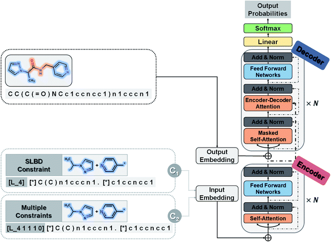
Our goal is to generate lead-like molecules by connecting pairs of fragments with constraints to the linker as shown in Fig. 1.There are two types of linking constraints used as control codes during training. One is the SLBD between two anchor points, which are used to maintain the relative position of a pair of fragments. The other one is the constraint with multiple features, such as the presence (1) or absence (0) of hydrogen bond donors (HBDs), hydrogen bond acceptors (HBAs), rotatable bonds (RBs) and rings, which can be regarded as additional pharmacophoric constraints.
This process can be regarded as an end-to-end sentence completion process, where a pair of fragments is the input signal and the full compound is the output signal. Schwaller et al.49 used encoder–decoder neural network architecture to predict reaction products in an end-to-end manner, where the reactants serve as the source sequence and the reaction product as the target sequence, whereas in our case, a pair of fragments and the constraints of the SLBD (as a prepended token) are defined as the source sequence, and the full molecule as the target sequence. Examples of the sequence expression are shown in Fig. 1. A training example with SLBD as the constraint is described as “[L_4]c1ccccc1[*].[*]C1CCOCC1 ≫ c1ccc(CNCC2CCOCC2)cc1”, where “[L_4]c1ccccc1[*].[*]C1CCOCC1” is the source sequence, “c1ccc(CNCC2CCOCC2)cc1” is the target sequence, and “[L_4]” is the SLBD (equal to four bond distance) as the control code. In the other example, “[L_4 1 1 1 0]” represents the multiple constraints, where “1 1 1 0” represents the presence of HBD, HBA, RB and the absence of a ring.
Throughout the study, SLBD only and SLBD plus multiple pharmacophore constraint model are named SyntaLinker and SyntaLinker_multi model respectively. Additionally, a reference model without using any constraint, SyntaLinker_n, was also trained for comparison.
Model architecture
A novel conditional generative model (SyntaLinker) with transformer architecture is proposed to generate molecular structures with user-defined conditions. Compared to the conventional transformer model,50 SyntaLinker (Fig. 2) introduces prepended control codes51,52 to the generated molecules complying with the user-defined criterion.All source and target sequences of our data set were first tokenized to construct a vocabulary. For each example sequence containing n tokens, where a token is referred to as an individual letter of the SMILES string, it was first encoded into a one-hot matrix by the vocabulary and then transformed into an embedding matrix Ms = (e1, …, en) by a word embedding algorithm53 as we did in our previous work.54Ms was composed of n corresponding vectors in Rd, where d is the embedding dimension.
The core architecture of SyntaLinker consists of multiple encoder–decoder stacks. The encoder and decoder consist of six identical layers. Each encoder layer has a multi-head self-attention sub-layer and a position-wise feedforward network (FFN) sub-layer. A multi-head attention consists of several scaled dot-product attention functions running in parallel and concatenates their outputs into final values, which allows the model to focus on information from different subspaces at different positions. An attention mechanism computes the dot products of the query (Q) with all keys (K), introduces a scaling factor dk (equal to the size of weight matrices) to avoid excessive dot products, and then applies a softmax function to obtain the weights on the values (V). Formally,
 | (1) |
For better understanding of the attention mechanism, we convert the mathematical expression in formula (1) into a chemically meaningful expression via a graphical illustration (as shown in Fig. S2†).
The FFN sub-layer adopts Rectified Linear Unit (ReLU) activation.55 Then, layer normalization56,57 and a residual connection58 are introduced to integrate the above two core sub-layers. Each decoder layer has three sub-layers, including two attention sub-layer and an FFN sub-layer. The decoder self-attention sub-layer uses a mask to preclude attending to future tokens, while the encoder–decoder attention sub-layer helps the decoder to focus on important characters in the source sequence, and capture the relationship between the encoder and decoder.
For a given source sequence, its input embedding is processed by encoder layers into a latent representation L = (l1, …, ln). Given L, the decoder output is normalized with a softmax function, yielding a probability distribution for sampling a token, and then generates an output sequence Y = y1, …, ym of one token at a time until the ending token “〈/s〉” is generated. Finally, the cross-entropy loss between the target sequence Mt = (e1, …, ek) and the output sequence Y is minimized during training.
 | (2) |
Data preparation
Our data were derived from the ChEMBL59 database and pre-processed in the same way as our previous study35 did, then filtered with Lipinski's “Rules of Five”,60 pan assay interference compounds7 (PAINS) substructures and, synthetic accessibility score61 (SAscore, the cut-off value set to 6.5) to guarantee that the generated molecules are lead-like and likely to be synthesizable.To mimic the fragment linking scenario, we constructed the data set using the matched molecular pairs (MMPs) cutting algorithm62 proposed by Hussain et al. Firstly, each molecule was deconstructed using the MMPs cutting algorithm, which executed double cuts of non-functional groups, acyclic single bonds in every compound and this will transform the compound into a quadruple form like “fragment 1, linker, fragment 2, molecule”, which corresponds to the two terminal fragments, a linker and the original compound. In total 5![[thin space (1/6-em)]](https://www.rsc.org/images/entities/char_2009.gif) 873
873![[thin space (1/6-em)]](https://www.rsc.org/images/entities/char_2009.gif) 503 fragment molecule quadruples (FMQs) were enumerated; secondly, the FMQs were further filtered using “Rule of three”63 criteria, i.e. an FMQ will be removed if any of its terminal fragment violates the “Rule of three” criteria; considering that the requirement of linking fragments in reality is to connect two close fragments using a linker as simple as possible, the remaining FMQs were then filtered by the SLBD of the linker (SLBD less than 15) and SAscore according to eqn (1) to ensure the terminal fragments have reasonable synthesis feasibility (SAscore is less than 5) and the SAscore of the linker is lower than the sum of the fragments, which can prevent the generation of highly complicated linkers. In our experience, applying these filters does help the generation of lead-like molecules.
503 fragment molecule quadruples (FMQs) were enumerated; secondly, the FMQs were further filtered using “Rule of three”63 criteria, i.e. an FMQ will be removed if any of its terminal fragment violates the “Rule of three” criteria; considering that the requirement of linking fragments in reality is to connect two close fragments using a linker as simple as possible, the remaining FMQs were then filtered by the SLBD of the linker (SLBD less than 15) and SAscore according to eqn (1) to ensure the terminal fragments have reasonable synthesis feasibility (SAscore is less than 5) and the SAscore of the linker is lower than the sum of the fragments, which can prevent the generation of highly complicated linkers. In our experience, applying these filters does help the generation of lead-like molecules.
 | (3) |
In the end, only terminal fragments and original compounds were kept as the fragment molecule triplet (FMT) for model training and all chemical structures in the FMTs were transformed to the canonicalized SMILES format46,64 with RDKit.65
Our ChEMBL data set was further divided into three sets with a ratio of 8![[thin space (1/6-em)]](https://www.rsc.org/images/entities/char_2009.gif) :
:![[thin space (1/6-em)]](https://www.rsc.org/images/entities/char_2009.gif) 1
1![[thin space (1/6-em)]](https://www.rsc.org/images/entities/char_2009.gif) :
:![[thin space (1/6-em)]](https://www.rsc.org/images/entities/char_2009.gif) 1 for training, validating, and testing, respectively. All FMTs were grouped by the corresponding SLBD. When splitting the ChEMBL set into those three sets, a random sampling strategy was adopted to make sure the distribution of SLBD is similar among all three sets.
1 for training, validating, and testing, respectively. All FMTs were grouped by the corresponding SLBD. When splitting the ChEMBL set into those three sets, a random sampling strategy was adopted to make sure the distribution of SLBD is similar among all three sets.
In addition, for further evaluating the generalization capability of our model, we also considered an external validation set derived from the CASF-2016 data set,66 which consists of 285 protein–ligand complexes with high-quality crystal structures.
Moreover, the SyntaLinker method was validated in three case studies derived from the literature to demonstrate the capability of fragment linking, lead optimization, and scaffold hopping. To make sure diverse structures are generated, only the SyntaLinker model was used in the case studies. It is worthwhile to mention that the ground truth compounds in these examples were not included in the training set of our SyntaLinker models.
Evaluation metrics for the SyntaLinker model
The ultimate goal of our model is to generate diverse molecules, containing a pair of fragments. Therefore, four different metrics on 2D level, validity, uniqueness, recovery and novelty, were employed to compare generated molecules and their ground truth in the test set.67,68 Here, validity refers to the percentage of generated chemically valid molecules with a pair of fragments; novelty is the percentage of generated chemically valid molecules with novel linkers (not present in the training set); uniqueness is the number of unique structures generated and recovery means the percentage of ground truth generated among test set compounds. Formally, | (4) |
 | (5) |
 | (6) |
The quality of compounds generated by the SyntaLinker model at the 3D level was also examined. In this case, the 3D conformations of compounds are generated and docked into protein binding pockets; the root mean square deviation (RMSD), and shape and colour combo-similarity score (SC) to the X-ray bound conformation of the actual ligand are generated to evaluate the model performance for selected cases. Here, RMSD is merely calculated among a pair of fragments of the X-ray and generated structures. The SC score is calculated by the pharmacophoric feature similarity69 and the shape similarity70 between the X-ray conformation of the actual ligand and the docking pose of the generated structure. The SC score is a real number in the range of [0,1] and the higher its value, the more similar the generated molecule is to the original ligand. For each molecule, the best similarity score among all docking conformers was taken as the SC score. In the current study, converting SMILES to the 3D conformation and docking were done by using the Molecular Operating Environment (MOE) software.71 The RMSD and SC score for each conformation were calculated via RDkit.65
Model training and optimization of hyperparameters
SyntaLinker was implemented in OpenNMT.72 All scripts were written in Python73 (version 3.7). We trained the models on GPU (Nvidia 2080Ti), and saved the checkpoint per 1000 steps. The best hyperparameters were obtained based on the recovery metric of the ChEMBL validation set. We built our model with the best hyperparameters (shown in Table S1†) and adopted the beam search procedure74 to generate multiple candidates with a special beam width. All generated candidates were canonicalized in RDkit and compared with the ground-truth molecules.Results and discussion
Eventually, we obtained 784![[thin space (1/6-em)]](https://www.rsc.org/images/entities/char_2009.gif) 728 FMQs from 718
728 FMQs from 718![[thin space (1/6-em)]](https://www.rsc.org/images/entities/char_2009.gif) 652 unique molecules from our data preparation process. As mentioned in the above section, three types of models were trained, i.e. SLBD only (SyntaLinker) and SLBD plus pharmacophore constraints (SyntaLinker_multi) and the reference model without using any constraint (SyntaLinker_n). The performance of our models on the ChEMBL test set and CASF validation set was examined. It is worth noting that the SyntaLinker method merely uses 2D molecular topology for model building, while the DeLinker method requires pre-generated three-dimensional conformations of a molecule as well as the relative 3D spatial information between fragments for creating the training set.
652 unique molecules from our data preparation process. As mentioned in the above section, three types of models were trained, i.e. SLBD only (SyntaLinker) and SLBD plus pharmacophore constraints (SyntaLinker_multi) and the reference model without using any constraint (SyntaLinker_n). The performance of our models on the ChEMBL test set and CASF validation set was examined. It is worth noting that the SyntaLinker method merely uses 2D molecular topology for model building, while the DeLinker method requires pre-generated three-dimensional conformations of a molecule as well as the relative 3D spatial information between fragments for creating the training set.
Model performance on the ChEMBL test set
We first validated the performance of SyntaLinker on the ChEMBL test set using 2D metrics. Top 10 candidates for each pair of starting fragments were generated. The results are listed in Table 1. All the models achieved over 95% validity, 90% linker novelty and recovered over 80% of the original molecules, demonstrating that the conditional transformer model can learn to identify the linker part of the structures, generate the linker accordingly, and also the models are generalized well enough to create new linkers. It seems that the constraint models are better than the model without using any constraint in terms of recovery, novelty and validity. Especially, the most detailed constraint model SyntaLinker_multi achieves a recovery rate of 87.1% in the top 10 recommendations. This is due to the fact that more prior knowledge about the linker is defined in the multiple constraint model than others.| Metrics | Models | ||
|---|---|---|---|
| SyntaLinker (%) | SyntaLinker_multi (%) | SyntaLinker_n (%) | |
| Validity | 97.2 | 97.8 | 96.0 |
| Uniqueness | 88.1 | 84.9 | 86.7 |
| Recovery | 84.7 | 87.1 | 80. |
| Novelty | 91.8 | 92.3 | 90.3 |
Model performance on CASF
To compare with the DeLinker model (downloaded from https://github.com/oxpig/DeLinker), we further evaluated the models on the external validation set CASF-2016,66 which was used in the DeLinker model. Following the same sampling strategy as DeLinker, we generated 250 molecules for each pair of starting fragments. The detailed performance of various models on the same validation set is listed in Table 2.| Metrics | Models | |||
|---|---|---|---|---|
| DeLinker (%) | SyntaLinker (%) | SyntaLinker_multi (%) | SyntaLinker_n (%) | |
| Validity | 95.5 | 96.4 | 96.5 | 86.8 |
| Uniqueness | 51.9 | 69.9 | 63.8 | 65.6 |
| Recovery | 53.7 | 62.7 | 60.2 | 55.4 |
| Novelty | 51.0 | 75.4 | 77.2 | 71.3 |
These metrics indicate that the performance of our models is significantly improved over the DeLinker model on the CASF validation set. Especially, our model improves the linker novelty of the DeLinker model by a margin of 20% without losing the recovery, meaning SyntaLinker can sample a diverse range of linkers more effectively.
Efficiency of controlling structure generation
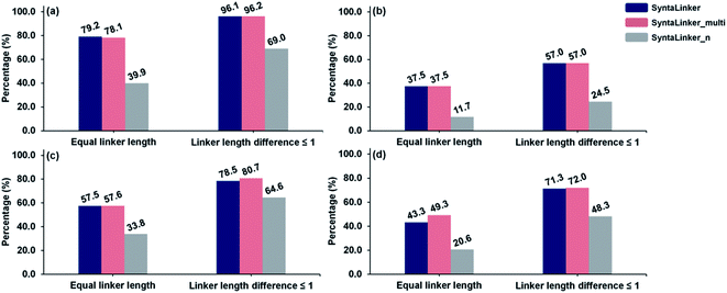
SyntaLinker aims to generate molecular structures that comply with the given criteria. We further calculated the SLBD and pharmacophore properties of the linkers in the generated molecules to verify whether these constraints were complied. The original linker bond length and pharmacophore properties of compounds in test sets were set as the control criterion when generating structures using the constrained model SyntaLinker and SyntaLinker_multi respectively, while SyntaLinker_n (unconstrained model) had no control criterion. For structures generated by all three models, the linker length and pharmacophore properties were examined for comparison purpose. Besides evaluating the control efficiency on the ChEMBL test set and CASF validation set, the effect of beam search width (top 10 and top 250) was also assessed.SLBD controlling efficiency of three SyntaLinker models on the ChEMBL test set in top 10 and top 250 are shown in Fig. 3a and b. They contain the percentage of structures with correct SLBD and structures whose SLBD variation is less than one bond distance. 79.2%, 78.1% and 39.9% of structures have exactly the same SLBD as the control for SyntaLinker, SyntaLinker_multi and SyntaLinker_n models respectively. That is, the models with length constraints (SyntaLinker, SyntaLinker_multi) outperform the model without constraints (SyntaLinker_n). Moreover, if SLBD is allowed to vary within one bond, then the percentage of structures complying the criteria from three models are 96.1%, 96.2% and 69% respectively.
For the CASF validation set, the same trend was observed in Fig. 3c. When we increase the beam search width from 10 to 250, the control efficiency of the shortest bond length for all three models will decrease (Fig. 3b and d). However, the conditional model still demonstrates superior performance to the one without condition restrictions.
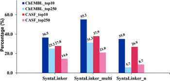
The percentage of structures with exactly equivalent pharmacophore properties to their ground truth from all three SyntaLinker models on the ChEMBL test set in top-10 and top-250 is depicted in Fig. 4. As expected, the model with pharmacophore constraints (SyntaLinker_multi) outperforms the model without this constraint (SyntaLinker, SyntaLinker_n), where 36.5%, 55.2% and 35.0% of structures have exactly the same pharmacophore properties as the control for SyntaLinker, SyntaLinker_multi and, SyntaLinker_n models on the ChEMBL test set. For the CASF validation set also the same trend was observed. Furthermore, when the beam search width was increased from 10 to 250, the control efficiency of the pharmacophore for all three models decreased. Due to the combination of multiple constraints, the control efficiency of pharmacophore constraints is lower than the one with the bond length constraint (Fig. 3). Nevertheless, the model with the constraints is superior to the model without constraints.
Properties of the generated molecules
To evaluate the quality of the generated molecules from SyntaLinker models, drug-likeness score (QED score), synthetic accessibility score (SAscore), the calculated water–octanol partition coefficient (log![[thin space (1/6-em)]](https://www.rsc.org/images/entities/char_2009.gif) P) and molecular weight (MW) were calculated using RDkit. For each pair of fragments in the ChEMBL test set, the properties of its top 10 and top 250 candidates were calculated and averaged to obtain a final value. A comparison with the properties of the original ChEMBL data (Fig. 5) showed that molecules generated from SyntaLinker models have significantly higher QED and lower SAscore values than the ones for ChEMBL compounds, suggesting that SyntaLinker generated molecules are more lead-like and have lower complexity for synthesis comparing with ChEMBL molecules. This is probably due to the fact that the chosen starting fragment pairs restraint the properties of the generated structures. The distributions of log
P) and molecular weight (MW) were calculated using RDkit. For each pair of fragments in the ChEMBL test set, the properties of its top 10 and top 250 candidates were calculated and averaged to obtain a final value. A comparison with the properties of the original ChEMBL data (Fig. 5) showed that molecules generated from SyntaLinker models have significantly higher QED and lower SAscore values than the ones for ChEMBL compounds, suggesting that SyntaLinker generated molecules are more lead-like and have lower complexity for synthesis comparing with ChEMBL molecules. This is probably due to the fact that the chosen starting fragment pairs restraint the properties of the generated structures. The distributions of log![[thin space (1/6-em)]](https://www.rsc.org/images/entities/char_2009.gif) P and MW are similar among ChEMBL and SyntaLinker generated molecules. Differences of all calculated properties among SyntaLinker models are trivial.
P and MW are similar among ChEMBL and SyntaLinker generated molecules. Differences of all calculated properties among SyntaLinker models are trivial.
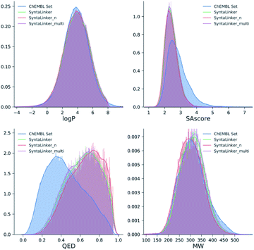 | ||
| Fig. 5 Distribution of chemical properties for ChEMBL molecules and the molecules generated from SyntaLinker models. | ||
Attention analysis
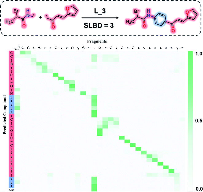
To investigate what the SyntaLinker has learned, we further analysed the attention weights for a linker generation example (as shown in Fig. 6). The attention weights provide clues on the importance of SMILES tokens in the input fragments for individual output character when the output sequence was generated. Fig. 6, for example, maps out the top candidate's attention weights extracted from the SyntaLinker model (with the SLBD constraint of 3), where the darker colour refers to larger importance of the character in the input. It is observed that in the left upper and right lower region of the attention map, diagonal cells obviously have larger weights, which corresponds to the high similarity between the SMILES substrings of input fragments and the terminal sections of the output structure. The attachment point token “[*]” has a very low weight, suggesting that it has a very low probability to be generated in the output structure. For the tokens in the linker part of the output structure, the token “.” in the input structure has larger weight than other tokens, which means the model recognizes the separation token between two fragments of the input structure and fills in the linker part in the correct place.In other words, the SyntaLinker model is able to identify the SMILES substrings for the terminal fragments of the input sequence and rearrange them correctly in the output sequence. Meanwhile, the breaking position in the input sequence can also be identified and the linker tokens are successfully added in, even though they are not arranged sequentially. As we can see that, in this example, an additional ring is created as the linker, ring number tokens can still be correctly assigned. This suggests that the SyntaLinker model has learned the implicit rules from the ChEMBL dataset and can nicely deal with both the local and global information during the structure generation.
Fragment linking case
Fragment linking aims to increase the affinity. For example, Trapero and colleagues identified phenylimidazole derivatives with low affinities against IMPDH through a virtual screening campaign. By linking fragments from original lead compound, they discovered a new molecule increased with more than 1000-fold binding affinity.75 Using the same fragments (PDB: 5OU2), we also generated the linked molecule (PDB: 5OU3) through the SyntaLinker model (Fig. 7). | ||
| Fig. 7 Fragment linking case study. (a) The binding poses of the pair of starting fragments (PDB: 5OU2). (b) The binding mode of the molecule generated by SyntaLinker (PDB: 5OU3). (c) The starting fragments and the linked molecule. | ||
Starting from the fragments in 5OU2 with the SLBD condition of 3 to 5, we generated 500 candidates with SyntaLinker. The native molecule (Fig. 7b) was successfully recovered and after 3D conformer generation and docking, most of the generated structures actually have a better docking score than the native molecule (Table 3). Three generated molecules with the highest 3D fragment similarity and favourable MOE docking scores are depicted in Fig. 8, where the native ligand binding poses are recovered by SyntaLinker (Fig. 8c).
| Metrics | Cases | ||
|---|---|---|---|
| Fragment linking | Lead optimization | ||
| Top 100 | Top 500 | Top 100 | |
| Unique structures | 47 | 341 | 808 |
| MOE score < lead | 35 | 306 | 107 |
| MOE score < −8.0 | 7 | 153 | 462 |
| MOE score < −9.0 | 1 | 22 | 22 |
| RMSD < 2.0 Å | 22 | 152 | 179 |
| SC > 0.5 | 9 | 36 | 44 |
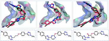 | ||
| Fig. 8 Overlays of the native ligand (PDB: 5OU3, green carbons) and three generated molecules (pink carbons, chemical structures shown in blue boxes) with the highest 3D fragment similarities and high MOE docking scores. | ||
Lead optimization case
Lead optimization is an iterative process of continuously modifying lead structures to improve potency and ADMET properties after initial lead compounds are identified. Here, we mimicked a typical lead optimization process via SyntaLinker. Dequalinium (Fig. 9c) has an inhibitory effect on chitinase A in the low nanomolar range (Ki: 70 nM), and is a promising lead against chitinase-mediated pathologies.76 Previous studies have demonstrated dequalinium's binding mode (PDB: 3ARP), and proven that linking two fragments (Fig. 9d) with a decane linker is critical, as it occupies the hydrophobic areas in the binding pocket.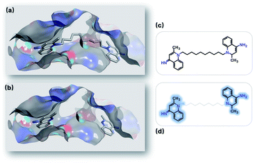 | ||
| Fig. 9 Optimizing leads by linking fragments. (a) Binding mode of chitinase A and dequalinium (PDB: 3ARP). (b) Binding modes of the two fragments derived from dequalinium. (c) Dequalinium structure. (d) Two fragments derived from dequalinium (marked in blue). | ||
To optimize dequalinium, we used the MMPs algorithm to derive fragment pairs from the molecule. This resulted in 45 non-redundant fragment pairs. They were used as terminal fragments for running SyntaLinker and 100 candidates were generated for each pair. The original linker bond length in dequalinium is set as the SLBD constraint for each pair. Dequalinium (native ligand) was recovered in these trials, and after removing redundant molecules, the RMSDs of two fragments were calculated. Details are also listed in Table 3.
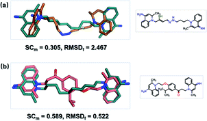
SyntaLinker can generate a large number of novel molecules. Among these molecules, 179 molecules have RMSD values less than 2 Å comparing with dequalinium, and 30 molecules have an RMSD value less than 1 Å comparing with dequalinium. For comparison, the best RMSD value for the top-5 molecules generated from DeLinker was 2.5 Å. Some molecules similar to dequalinium (the lead) are depicted in Fig. 10. Fig. 11 lists three molecules generated by SyntaLinker and their RMSD values in comparison with dequalinium structure. Our SyntaLinker model seems to give chemically reasonable compounds (three examples are shown in Fig. 11) and also better RMSD and SC metrics. This may be because chemically more attractive linkers existed in our ChEMBL training set and also the ease of learning chemical syntactics by a sequence generation model comparing with the graph generation model.
 | ||
| Fig. 11 Three molecules generated by SyntaLinker and their RMSD values in comparison with dequalinium structure. | ||
Scaffold hopping case
Scaffold hopping aims to explicitly change the scaffold topology while still preserving the biological activity. In this study, to test the scaffold hopping capacity of SyntaLinker, two JNK3 inhibitors, indazole (PDB: 3FI3) and aminopyrazole (PDB: 3FI2) derivatives, were used as examples.77 Both inhibitors have almost the same binding modes as JNK3 (Fig. 12). | ||
| Fig. 12 Scaffold of JNK3 inhibitors. (a) Overlay of the indazole (PDB: 3FI3, green) and aminopyrazole (PDB: 3FI2, pink) structures. (b) Chemical structure and Murcko scaffold of the indazole (upper) and aminopyrazole (down) compounds. The highlighted substructures are fragmental pairs for linking. | ||
SyntaLinker generated 2500 molecules with the restriction of SLBD ranging from 6 to 8. This resulted in 2138 non-redundant molecules, in which more than thousand molecules had RMSD values less than 1 Å and SC values greater than 0.5. 634 linkers are novel (not found in the training set) covering 186 unique Murcko scaffolds.78 Both indazole (Fig. 13a) and aminopyrazole native molecules (Fig. 13b) were also recovered. This result highlights that our SyntaLinker model is well generalized to design novel linkers by combining the chemical information of starting fragments, not merely remembering the linkers in the ChEMBL training set.
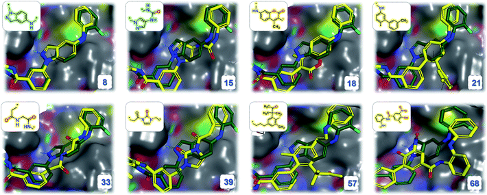 | ||
| Fig. 13 Overlay of the indazole inhibitor (PDB: 3FI3, green) and several example structures (yellow) with high 3D similarity. The linker structures are shown (novel scaffolds are coloured yellow, the recovered ground truth scaffolds are coloured green) in the upper left, and the order numbers (sorted by the SC score) are shown in the bottom right. | ||
Fig. 13 demonstrates the binding modes for eight generated structures with novel scaffolds. These new molecules are superimposed nicely with the native ligand.
Conclusions
Conventional fragment linking paradigm requires pre-defining a set of fragments (aka substructures or chemotypes) and then, assembling them into molecules with rigid transformation rules or reaction rules. By implementing SyntaLinker, we prove that linking fragments can be accomplished by the syntactic pattern recognition technique. We used deep transformer neural networks to learn the implicit rules of linking fragments among ChEMBL compounds by recognizing syntactic patterns embedded in SMILES. Our results demonstrate that the SyntaLinker model is able to generate molecular structures based on a given pair of fragments and additional restrictions. The attention map analysis shows that the transformer model can successfully recognize the terminal fragments in the input sequence, learn the implicit rules in generating linkers, as well as assemble these substructures together. Furthermore, SyntaLinker can be used in drug design processes, such as virtual library construction from fragments, lead optimization, and scaffold hopping, as we have demonstrated in this work.Notes
The source code and data of SyntaLinker are available online at https://github.com/YuYaoYang2333/SyntaLinker.Conflicts of interest
There are no conflicts to declare.Acknowledgements
This work was funded in part of the National Key R&D Program of China (2017YFB0203403), the Science and Technology Program of Guangzhou (201604020109), the Guangdong Provincial Key Lab. of New Drug Design and Evaluation (Grant 2011A060901014).References
- R. Macarron, M. N. Banks, D. Bojanic, D. J. Burns, D. A. Cirovic, T. Garyantes, D. V. S. Green, R. P. Hertzberg, W. P. Janzen, J. W. Paslay, U. Schopfer and G. S. Sittampalam, Nat. Rev. Drug Discovery, 2011, 10, 188–195 CrossRef CAS PubMed.
- D. J. Ecker and S. T. Crooke, Biotechnol., 1995, 13, 351–360 CAS.
- P. J. Hajduk and J. Greer, Nat. Rev. Drug Discov., 2007, 6, 211–219 CrossRef CAS PubMed.
- D. Fattori, A. Squarcia and S. Bartoli, Drugs R, 2008, 9, 217–227 CrossRef CAS PubMed.
- K. H. Bleicher, H.-J. Böhm, K. Müller and A. I. Alanine, Nat. Rev. Drug Discovery, 2003, 2, 369–378 CrossRef CAS PubMed.
- C. W. Murray and D. C. Rees, Nat. Chem., 2009, 1, 187–192 CrossRef CAS PubMed.
- J. B. Baell and G. A. Holloway, J. Med. Chem., 2010, 53, 2719–2740 CrossRef CAS PubMed.
- A. Jadhav, R. S. Ferreira, C. Klumpp, B. T. Mott, C. P. Austin, J. Inglese, C. J. Thomas, D. J. Maloney, B. K. Shoichet and A. Simeonov, J. Med. Chem., 2010, 53, 37–51 CrossRef CAS PubMed.
- P. J. Hajduk, Nat. Chem. Biol., 2006, 2, 658–659 CrossRef CAS PubMed.
- P. J. Hajduk, J. Med. Chem., 2006, 49, 6972–6976 CrossRef CAS PubMed.
- M. Baker, Nat. Rev. Drug Discovery, 2013, 12, 5–10 CrossRef CAS PubMed.
- W. P. Jencks, Proc. Natl. Acad. Sci. U. S. A., 1981, 78, 4046–4050 CrossRef CAS PubMed.
- D. A. Erlanson, S. W. Fesik, R. E. Hubbard, W. Jahnke and H. Jhoti, Nat. Rev. Drug Discovery, 2016, 15, 605–619 CrossRef CAS PubMed.
- T. G. Davies and I. J. Tickle, in Fragment-Based Drug Discovery and X-Ray Crystallography, ed. T. G. Davies and M. Hyvönen, Springer Berlin Heidelberg, Berlin, Heidelberg, 2012, pp. 33–59, DOI:10.1007/128_2011_179.
- H. Chen, X. Zhou, A. Wang, Y. Zheng, Y. Gao and J. Zhou, Drug Discov. Today, 2015, 20, 105–113 CrossRef CAS PubMed.
- W. Zhang, Med. Res. Rev., 2013, 33, 554–598 CrossRef PubMed.
- D. Joseph-McCarthy, A. J. Campbell, G. Kern and D. Moustakas, J. Chem. Inf. Model., 2014, 54, 693–704 CrossRef CAS PubMed.
- H. Chen, L. Knerr, T. Åkerud, K. Hallberg, L. Öster, M. Rohman, K. Österlund, H.-G. Beisel, T. Olsson, J. Brengdhal, J. Sandmark and C. Bodin, Bioorg. Med. Chem. Lett., 2014, 24, 5251–5255 CrossRef CAS PubMed.
- D. C. Rees, Annu. Rep. Med. Chem., 2007, 42, 431–448 Search PubMed.
- H. Möbitz, R. Machauer, P. Holzer, A. Vaupel, F. Stauffer, C. Ragot, G. Caravatti, C. Scheufler, C. Fernandez, U. Hommel, R. Tiedt, K. S. Beyer, C. Chen, H. Zhu and C. Gaul, ACS Med. Chem. Lett., 2017, 8, 338–343 CrossRef PubMed.
- S. B. Shuker, P. J. Hajduk, R. P. Meadows and S. W. Fesik, Science, 1996, 274, 1531 CrossRef CAS PubMed.
- A. Medek, P. J. Hajduk, J. Mack and S. W. Fesik, J. Am. Chem. Soc., 2000, 122, 1241–1242 CrossRef CAS.
- M. Mondal, N. Radeva, H. Fanlo-Virgós, S. Otto, G. Klebe and A. K. H. Hirsch, Angew. Chem., Int. Ed. Engl., 2016, 55, 9422–9426 CrossRef CAS PubMed.
- V. Borsi, V. Calderone, M. Fragai, C. Luchinat and N. Sarti, J. Med. Chem., 2010, 53, 4285–4289 CrossRef CAS PubMed.
- J. D. Chodera and D. L. Mobley, Annu. Rev. Biophys., 2013, 42, 121–142 CrossRef CAS PubMed.
- O. Ichihara, J. Barker, R. J. Law and M. Whittaker, Mol. Inform., 2011, 30, 298–306 CrossRef CAS PubMed.
- M. Glick, J. Med. Chem., 2008, 51, 2481–2491 CrossRef PubMed.
- S. Chung, J. B. Parker, M. Bianchet, L. M. Amzel and J. T. Stivers, Nat. Chem. Biol., 2009, 5, 407–413 CrossRef CAS PubMed.
- D. G. Fedorov and K. Kitaura, J. Comput. Chem., 2007, 28, 222–237 CrossRef CAS PubMed.
- K. Kitaura, E. Ikeo, T. Asada, T. Nakano and M. Uebayasi, Chem. Phys. Lett., 1999, 313, 701–706 CrossRef CAS.
- D. G. Fedorov and K. Kitaura, J. Phys. Chem. A, 2007, 111, 6904–6914 CrossRef CAS PubMed.
- H. Chen, O. Engkvist, Y. Wang, M. Olivecrona and T. Blaschke, Drug Discov. Today, 2018, 23, 1241–1250 CrossRef PubMed.
- Y. Xu, K. Lin, S. Wang, L. Wang, C. Cai, C. Song, L. Lai and J. Pei, Future Med. Chem., 2019, 11, 567–597 CrossRef CAS PubMed.
- D. C. Elton, Z. Boukouvalas, M. D. Fuge and P. W. Chung, CoRR, 2019, arXiv:abs/1903.04388 Search PubMed.
- M. Olivecrona, T. Blaschke, O. Engkvist and H. Chen, J. Cheminf., 2017, 9, 48 Search PubMed.
- M. H. S. Segler, T. Kogej, C. Tyrchan and M. P. Waller, CoRR, 2017, arXiv:abs/1701.01329 Search PubMed.
- R. Gómez-Bombarelli, D. Duvenaud, J. M. Hernández-Lobato, J. Aguilera-Iparraguirre, T. D. Hirzel, R. P. Adams and A. Aspuru-Guzik, CoRR, 2016, arXiv:abs/1610.02415 Search PubMed.
- O. Prykhodko, S. V. Johansson, P.-C. Kotsias, J. Arús-Pous, E. J. Bjerrum, O. Engkvist and H. Chen, J. Cheminf., 2019, 11, 74 Search PubMed.
- W. Jin, K. Yang, R. Barzilay and T. S. Jaakkola, CoRR, 2018, arXiv:abs/1812.01070 Search PubMed.
- Z. Zhou, S. M. Kearnes, L. Li, R. N. Zare and P. Riley, CoRR, 2018, arXiv:abs/1810.08678 Search PubMed.
- T. Fu, C. Xiao and J. Sun, 2020, arXiv:abs/1912.05910.
- T. Mikolov, M. Karafiát, L. Burget, J. Černocký and S. Khudanpur, INTERSPEECH, 2010 Search PubMed.
- D. P. Kingma and M. Welling, CoRR, 2014, arXiv:abs/1312.6114 Search PubMed.
- A. Makhzani, J. Shlens, N. Jaitly and I. J. Goodfellow, 2015, arXiv:abs/1511.05644.
- I. J. Goodfellow, J. Pouget-Abadie, M. Mirza, B. Xu, D. Warde-Farley, S. Ozair, A. C. Courville and Y. Bengio, 2014, arXiv:abs/1406.2661.
- D. Weininger, J. Chem. Inf. Comput. Sci., 1988, 28, 31–36 CrossRef CAS.
- F. Imrie, A. R. Bradley, M. van der Schaar and C. M. Deane, J. Chem. Inf. Model., 2020, 60, 1983–1995 CrossRef CAS PubMed.
- G. Zweig, J. C. Platt, C. Meek, C. J. C. Burges, A. Yessenalina and Q. Liu, presented in part at the Proceedings of the 50th Annual Meeting of the Association for Computational Linguistics: Long Papers - Volume 1, Jeju Island, Korea, 2012 Search PubMed.
- P. Schwaller, T. Gaudin, D. Lányi, C. Bekas and T. Laino, Chem. Sci., 2018, 9, 6091–6098 RSC.
- A. Vaswani, N. Shazeer, N. Parmar, J. Uszkoreit, L. Jones, A. N. Gomez, L. Kaiser and I. Polosukhin, CoRR, 2017, arXiv:abs/1706.03762 Search PubMed.
- C. W. Pfaff, Language, 1979, 55, 291–318 CrossRef.
- P. Shana, Linguistics, 1980, 18, 581–618 Search PubMed.
- T. Chen, R. Xu, Q. Lu, B. Liu, J. Xu, L. Yao and Z. He, Computational Linguistics and Intelligent Text Processing, Berlin, Heidelberg, 2014 Search PubMed.
- S. Su, Y. Yang, H. Gan, S. Zheng, F. Gu, C. Zhao and J. Xu, J. Chem. Inf. Model., 2020, 60, 1165–1174 CrossRef CAS PubMed.
- V. Nair and G. E. Hinton, presented in part at the ICML, 2010 Search PubMed.
- J. Ba, J. R. Kiros and G. E. Hinton, 2016, arXiv:abs/1607.06450.
- L. Barrault, O. e. Bojar, M. R. Costa-jussà, C. Federmann, M. Fishel, Y. Graham, B. Haddow, M. Huck, P. Koehn, S. Malmasi, C. Monz, M. Müller, S. Pal, M. Post and M. Zampieri, presented in part at the Proceedings of the Fourth Conference on Machine Translation Volume 2: Shared Task Papers, Day 1, Florence, Italy, 2019 Search PubMed.
- K. He, X. Zhang, S. Ren and J. Sun, CoRR, 2015, arXiv:abs/1512.03385 Search PubMed.
- A. Gaulton, L. J. Bellis, A. P. Bento, J. Chambers, M. Davies, A. Hersey, Y. Light, S. McGlinchey, D. Michalovich, B. Al-Lazikani and J. P. Overington, Nucleic Acids Res., 2011, 40, D1100–D1107 CrossRef PubMed.
- C. Lipinski and A. Hopkins, Nature, 2004, 432, 855–861 CrossRef CAS PubMed.
- P. Ertl and A. Schuffenhauer, J. Cheminf., 2009, 1, 8 Search PubMed.
- J. Hussain and C. Rea, J. Chem. Inf. Model., 2010, 50, 339–348 CrossRef CAS PubMed.
- H. Jhoti, G. Williams, D. C. Rees and C. W. Murray, Nat. Rev. Drug Discovery, 2013, 12, 644 CrossRef CAS PubMed.
- D. Weininger, A. Weininger and J. L. Weininger, J. Chem. Inf. Comput. Sci., 1989, 29, 97–101 CrossRef CAS.
- G. Landrum, RDKit: Open-source cheminformatics, accessed December 20, 2018, http://www.rdkit.org Search PubMed.
- M. Su, Q. Yang, Y. Du, G. Feng, Z. Liu, Y. Li and R. Wang, J. Chem. Inf. Model., 2019, 59, 895–913 CrossRef CAS PubMed.
- N. Brown, M. Fiscato, M. H. S. Segler and A. C. Vaucher, J. Chem. Inf. Model., 2019, 59, 1096–1108 CrossRef CAS PubMed.
- D. Polykovskiy, A. Zhebrak, B. Sanchez-Lengeling, S. Golovanov, O. Tatanov, S. Belyaev, R. Kurbanov, A. Artamonov, V. Aladinskiy, M. Veselov, A. Kadurin, S. I. Nikolenko, A. Aspuru-Guzik and A. Zhavoronkov, CoRR, 2018, arXiv:abs/1811.12823 Search PubMed.
- S. Putta, G. A. Landrum and J. E. Penzotti, J. Med. Chem., 2005, 48, 3313–3318 CrossRef CAS PubMed.
- G. A. Landrum, J. E. Penzotti and S. Putta, J. Comput.-Aided Mol. Des., 2006, 20, 751–762 CrossRef CAS PubMed.
- MOE, Chemical Computing Group, 1010 Sherbrooke St. W, Suite 910, Montreal, Quebec, Canada H3A 2R7, accessed February 16, 2020, http://www.chemcomp.com.
- G. Klein, Y. Kim, Y. Deng, J. Senellart and A. M. Rush, CoRR, 2017, arXiv:abs/1701.02810 Search PubMed.
- Python Core Team, Python: A dynamic, open source programming language, Python Software Foundation, http://https://www.python.org/ Search PubMed.
- P. S. Ow and T. E. Morton, Int. J. Prod. Res., 1988, 26, 35–62 CrossRef.
- A. Trapero, A. Pacitto, V. Singh, M. Sabbah, A. G. Coyne, V. Mizrahi, T. L. Blundell, D. B. Ascher and C. Abell, J. Med. Chem., 2018, 61, 2806–2822 CrossRef CAS PubMed.
- S. Pantoom, I. R. Vetter, H. Prinz and W. Suginta, J. Biol. Chem., 2011, 286, 24312–24323 CrossRef CAS PubMed.
- T. Kamenecka, J. Habel, D. Duckett, W. Chen, Y. Y. Ling, B. Frackowiak, R. Jiang, Y. Shin, X. Song and P. LoGrasso, J. Biol. Chem., 2009, 284, 12853–12861 CrossRef CAS PubMed.
- G. W. Bemis and M. A. Murcko, J. Med. Chem., 1996, 39, 2887–2893 CrossRef CAS PubMed.
Footnotes |
| † Electronic supplementary information (ESI) available. See DOI: 10.1039/d0sc03126g |
| ‡ These authors contributed equally. |
| This journal is © The Royal Society of Chemistry 2020 |


