The TensorMol-0.1 model chemistry: a neural network augmented with long-range physics

Abstract

Traditional force fields cannot model chemical reactivity, and suffer from low generality without re-fitting. Neural network potentials promise to address these problems, offering energies and forces with near ab initio accuracy at low cost. However a data-driven approach is naturally inefficient for long-range interatomic forces that have simple physical formulas. In this manuscript we construct a hybrid model chemistry consisting of a nearsighted neural network potential with screened long-range electrostatic and van der Waals physics. This trained potential, simply dubbed “TensorMol-0.1”, is offered in an open-source Python package capable of many of the simulation types commonly used to study chemistry: geometry optimizations, harmonic spectra, open or periodic molecular dynamics, Monte Carlo, and nudged elastic band calculations. We describe the robustness and speed of the package, demonstrating its millihartree accuracy and scalability to tens-of-thousands of atoms on ordinary laptops. We demonstrate the performance of the model by reproducing vibrational spectra, and simulating the molecular dynamics of a protein. Our comparisons with electronic structure theory and experimental data demonstrate that neural network molecular dynamics is poised to become an important tool for molecular simulation, lowering the resource barrier to simulating chemistry.

---

1 Introduction

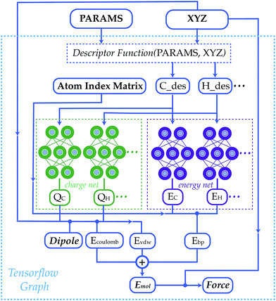
Statistical models from machine learning experienced growing popularity in many areas of chemistry, such as in reducing the cost of simulating chemical systems,^1–13 improving the accuracy of quantum methods,^14–22 generating force field parameters,^23,24 predicting molecular properties^25–32 and designing new materials.^33–38 Neural network model chemistries (NNMCs) are one of the most powerful methods among this class of models.^39–45 They are shown to be capable of generating high quality potential energy surfaces (PESs) with different schemes such as summing over atoms or bonds,^46–57 many-body expansions^58–60 and permutation invariant polynomials.^61–64 They are also used to predict the properties of materials,^65–73 and even to find new drugs.^74–79 In spite of their growing popularity, traditional force fields remain more popular than NNMCs, even for screening and reactive applications. This paper develops an open-source, transferable neural network model chemistry called TensorMol-0.1 (Fig. 1). This model hybridizes a NNMC with the physical contributions to molecular energies that are familiar from Molecular Mechanics and corrections to Density Functional Theory (DFT).⁸⁰ This approach yields a predictable reproduction of physical long-range forces, and features a linear-scaling inductive charge model. The charges do not depend on a quadratic-scaling polarization equation like a Thole-model,⁸¹ instead they are not fixed and respond well to geometry changes as we will show with reproduction of IR spectra.

Fig. 1 A schematic graph of TensorMol-0.1. Each element has its own charge network and energy network. The charge network predicts the atomic charges that yield the ab initio dipole moment. An atom index matrix is used to reassemble the molecular energies/dipoles from atom energies/charges. The Behler–Parinello type energy network produces a short-range embedded atomic energy, which is summed with the electrostatic energy and van der Waals energy to predict the total atomization energy of molecules at and away from equilibrium.

Our group is one of several who have been pursuing transferable and black-box neural network model chemistries.^{7,16,46,50,54,82,83} The state of the art in this field is progressing rapidly. Readers may not appreciate that a model can achieve chemical accuracy for energies but have uselessly noisy forces. Models that provide energies at equilibrium, and those treating a fixed molecule or stoichiometry, are nowadays reliably produced.⁵⁰ We will show that TensorMol-0.1 yields usefully accurate predictions of forces out-of-equilibrium by showing the reproduction of infrared spectra that closely approximate our source model chemistry (ωB97X-D, 6-311G**),⁸⁴ and molecular dynamics. We outline several tricks that are required to ensure the stability of long-time molecular dynamics.

This force model is implemented in an open-source package that uses the TensorFlow tensor algebra system to compute descriptors and forces. The methodology can be used to propagate the dynamics of large molecules (10⁵ atoms) on simple laptop computers. No force field refinement, atom assignment, or other interventions are needed to apply the method to a molecule of interest, so long as the elements are supported. The package is also interfaced with the I-PI path integral package,⁸⁵ to allow for quantum simulations and enhanced sampling.

2 Methods

The community of neural network model chemistry developers is rapidly improving the accuracy and generality of these reactive force fields.^{4,48,49,63,82,86} The model developed in this paper includes several components that were the subject of recent developments in other groups.^{46,49,52,82,87} We will describe the details here from the bottom up, citing prior studies. Our notational convention will be that i, j, k… are the indices of atoms, q_i is the charge on atom i, x, y and z are atomic numbers, A, B and C are molecules, and α, β… are the indices of basis functions which are the products of radial and angular functions. If a function depends on all the atomic coordinates of a molecule it will be written as a vector, and those functions which depend on only a few coordinates will be given explicit indices. The energy of TensorMol-0.1 is expressed as a sum of a short-range embedded n-body potential,⁴⁹ long-range electrostatic potential and van der Waals force:

In the above expression E_zi is a Behler–Parinello type energy network for the element z for atom i. This n-body potential takes as its argument S_α, the modified symmetry functions of Isayev and coworkers:⁸²

Modern machine learning frameworks provide automatic differentiation of tensor algebraic expressions, allowing a force field developer to obtain the gradient of a molecular potential in a single line of code, once the expression for E(R⃑) has been written. An important feature of our code is that this symmetry function is coded within the TensorFlow system,⁸⁸ so all the parameters of this descriptor can be optimized alongside the network weights to minimize error. Our implementation of the symmetry function employs a list of nearest-pairs and triples within radial cutoffs such that the scaling of the overall network is asymptotically linear. On an ordinary laptop equipped with only a CPU, a force/energy call on 20 000 atoms takes less than a minute.

The second term of our energy expression is the damped-shifted force (DSF) Coulomb energy of Gezelter and coworkers.⁸⁹ The charges are obtained from a sub-network which reproduces molecular dipole moments. Previous studies^90,91 included electrostatic energy by training the networks to learn Hirshfeld charges. Our charge model enforces conservation of total charge by evenly spreading any required neutralizing charge over the entire molecule or unit cell. The damped-shifted force ensures the long range continuity and differentiability of the effective Coulomb potential with smooth cutoffs. We modify the DSF kernel at short range with an “elu” type non-linearity,⁹² such that the forces within the radius of the Behler–Parinello symmetry function smoothly approach zero, avoiding singularities and interference with the Behler–Parinello many-body potential. The range separation concept has a long history in chemistry whenever two models of a physical force have complementary cost or accuracy range advantages.⁸⁴ The energy of the DSF kernel is expressed as:

where E_{DSF(original)} is the energy of the DSF kernel⁸⁹ and R_switch is the short range cutoff for the “elu” kernel. α_elu and β_elu are chosen so that the value and the gradient of E_DSF are continuous at R_switch. The damped-shifted force is well-suited to being combined with neural network models because it requires no Fourier transformation to treat periodic systems with linear scaling, and maps well onto TensorFlow. The last term is the van der Waals energy, which is calculated by following Grimme’s C6 scheme.⁸⁰

We employed a two step training approach. First, the charge networks are trained to learn the atom charges that predict the dipole moment. The loss function can be written as follows:

After the charge training is converged, we train the energy network. During the energy network training, the weights in charge networks are kept frozen, but they are still evaluated to calculate the electrostatic energy that is added to construct the total energy. Our Behler–Parinello many-body potential also absorbs the shape of the transition between the many-body and electrostatic regions. The learning target for the energy network includes both the DFT energy and DFT force. The loss function for the energy network training is:

where E^NN is obtained according to eqn (1) and F^NN is calculated by taking the gradient of E^NN with respect to the coordinates of the atoms. N_atom is the number of the atoms in the system and γ is a parameter that controls the portion of force loss. We employ γ = 0.05. We trained two neural networks based on two sets of data (see Table 1). One network (the “water network”) was trained on a database that includes ∼370 000 water clusters with 1 to 21 water molecules. The other network was trained on ∼3 000 000 different geometries of ∼15 000 different molecules that only contain C, H, O and N and up to 35 atoms. Since these 15 000 molecules were sampled randomly from the Chemspider database, we will refer to this network as the “Chemspider network” in the following text. The training geometries were sampled with metadynamics⁹³ and their energies calculated using the QChem⁹⁴ program and ωB97X-D⁸⁴ exchange correlation functional and a 6-311G** basis set.

Table 1 Training details and test RMSE of each learning target. The unit of energy RMSE, gradient RMSE and dipole RMSE is kcal mol⁻¹ per atom, kcal mol⁻¹ Å⁻¹ per atom and Debye per atom, respectively

	Water network	Chemspider network
a Training was done on a single Nvidia K40 GPU
Number of training cases	370 844	2 979 162
Training time (days)^a	3	10
Energy RMSE	0.054	0.24
Gradient RMSE	0.49	2.4
Dipole RMSE	0.0082	0.024

---

Each charge network and energy network contains three fully-connected hidden layers with 500 hidden neurons in each layer. For the Chemspider network, a network with three hidden layers, with 2000 hidden neurons in each layer, is used for each charge network and energy network. L2 regularization is used for both networks and dropout⁹⁵ on the last layer was used for the Chemspider network to prevent overfitting, with a dropout probability of 0.3. We chose a soft-plus function (ln(1.0 + e^αx)/α) with α = 100 as the non-linear activation function and used the Adaptive moment solver (Adam)⁹⁶ to fix the weights of the network. The test sets were separated from the training data by randomly choosing 20% of the molecules at the outset, which were kept independent throughout. Besides water, we will present calculations from molecules strictly absent from either the training or test set.

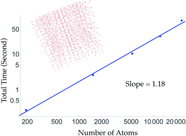
To obtain linear scaling, TensorMol uses atom neighbor lists within cutoffs. This allows double precision energy, charge and force calculations of up to 24 000 atoms to be executed in less than 90 seconds on a 2015 Intel i7 2.5 GHz MacBook Pro (Fig. 2). Periodic evaluations are achieved by tessellation of a unit cell with summation of the energies of atoms within the cell. Periodic calculations require about three times more wall time to execute. Speedups greater than a factor of two are obtained automatically when using computers with GPUs (Fig. S7†) or single-precision calculations.

Fig. 2 Aperiodic timings of an energy, charge and force call for cubic water clusters at a density of 1 g cm⁻³. The largest ∼60 Angstrom cube is 4× larger than the electrostatic cutoff. The slope of a log–log version of this curve is near unity, indicating the wall-time scaling of TensorMol. Inset figure: the cubic water cluster used for timing containing 1728 water molecules.

3 Results

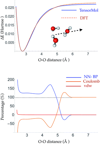
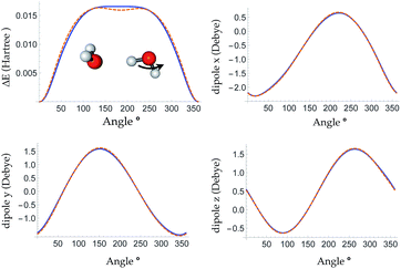
The root mean square error (RMSE) on the independent test set of the energy is 0.054 kcal mol⁻¹ atom⁻¹ and the RMSE of the force is 0.49 kcal mol⁻¹ Å⁻¹. The top panel of Fig. 3 is a plot of the potential energy surface (PES) of a water trimer when one of the water molecules is pulled away from the other two. One can see our neural network PES is not only in good agreement with the PES of the target method but is also smooth. To achieve this we use a variation of the soft-plus neuron rather than the rectified linear units that are popular in computer science. The latter train more efficiently, but produce discontinuous forces.

Fig. 3 Top panel: the PES of a water trimer when one water is pulled away from the other two. Bottom panel: the percentage contribution of the Behler–Parrinello atom-wise energy, electrostatic energy and van der Waals energy to the binding energy between the water that is pulled away and the other two waters. The Behler–Parrinello atom-wise energy contributes most of the binding energy at short range and the electrostatic energy is the dominant contribution at long range.

The bottom panel shows the fractional contribution of each of the three energy components in eqn (1) to the binding energy along the trimer dissociation coordinate. At short range, most of the binding energy is contributed by the n-body neural network potential. When the distance between the monomer and the dimer approaches the cutoff distance of the neural network, the contribution of the neural network potential starts to decrease and the contribution of the electrostatic potential increases. After 6 Å, where the neural network symmetry functions on the atoms in the monomer have no contribution from the dimer, the neural network force drops smoothly to zero and the electrostatic interaction dominates. The small difference in the energy at 7 Å is due to the difference between the Madelung energy given by the learned charges, and the genuine physical cohesive forces at this distance. The dimer and monomer are beyond the symmetry function sensory radius, and so the charges are constant in this region. Future iterations of the charge network will use local-field information to improve this region of the PES. The learned inductive charges are of high quality considering their linear scaling cost. Fig. 4 shows the PES and dipole change of a water dimer when the hydrogen bond is broken by rotating the OH bond. Both the PES and dipole change fit well with the DFT results.

Fig. 4 Top left panel: the PES of breaking a hydrogen bond between two waters by rotating one water around the O–H bond. Top right, bottom left and bottom right panels: change in the x, y and z dipole components during the rotation, respectively. DFT (ωB97X-D/6-311G**) results are shown in dashed orange line and the TensorMol force field results are plotted in solid blue line.

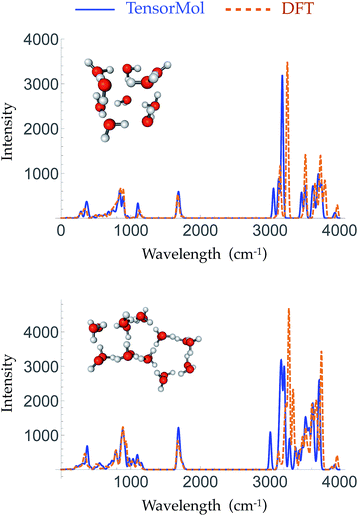
Given the increased dimensions of the Hessian, it is naturally a more stringent test to reproduce forces and infrared spectra than it is to simply produce energies. The top panel and bottom panel of Fig. 5 show the optimized geometries and IR spectra of a 10 water cluster and a 20 water cluster, respectively, generated using our force field and DFT. Each method uses its own equilibrium geometry, so this also tests the ability of TensorMol-0.1 to reproduce non-covalent geometries. Our force field quantitatively reproduces the IR spectra generated using DFT, both in terms of frequencies and intensities, especially for the water bend modes and inter-monomer modes. The Mean Absolute Error (MAE) of the frequencies in those two regions is 33.2 cm⁻¹ for the 10 water cluster and 16.2 cm⁻¹ for the 20 water cluster. The error is slightly larger in the water OH stretching region with a MAE of 34.2 cm⁻¹ and 13.1 cm⁻¹ for the 10 and 20 water clusters, respectively. This accuracy is comparable to high quality polarizable water force fields.⁶

Fig. 5 The simulated harmonic IR spectra of a 10 water cluster (top panel) and a 20 water cluster (bottom panel) generated using ωB97X-D/6-311G** (dashed orange line) and the TensorMol force field (solid blue line).

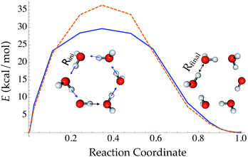
Compared with traditional force fields, one major advantage of TensorMol is its reactivity. TensorMol is able to simulate a concerted proton transfer in a water hexamer, finding a minimum energy transition path. The PES calculated using a nudged elastic band (NEB) method⁹⁷ with the TensorMol force field and the PES calculated using DFT are shown in Fig. 6. The barrier height predicted by TensorMol is 29.7 kcal mol⁻¹, which is 6.7 kcal mol⁻¹ lower than the prediction from DFT, which is remarkable considering the dearth of transition structures in the training data. Our method of sampling molecular geometries uses a meta-dynamics procedure described elsewhere,⁹³ so these proton transfers do occur in the training data although extremely infrequently.

Fig. 6 The reaction energy profile converged from a nudged elastic band method along the reaction coordinate of conservative proton transfer in a water hexamer cluster. The reaction coordination is defined as (R_OH − R_ini)/(R_final − R_ini).

Encouraged by our results from studying water, we developed a force field with applicability across the chemical space spanned by C, N, O and H. The Chemspider dataset that we used to train our force field covers a vast area of chemical space containing 15 thousand different molecules and 3 million geometries. The geometries are generated using a meta-dynamics procedure,⁹⁸ which ensures that each new geometry is a fresh part of chemical space; energies up to 400k_bT are sampled in the data. We describe the details of this meta-dynamics sampling algorithm, which we have found vital to achieving robust and transferable force fields elsewhere.⁹³ The diversity of structures makes learning the Chemspider dataset a much harder task for the TensorMol-0.1 network; the test set RMSE of energy is 0.24 kcal mol⁻¹ atom⁻¹ and the RMSE of force is 2.4 kcal mol⁻¹ atom⁻¹. More importantly, the model usefully reproduces several elements of molecular structures, at and away from equilibrium, for molecules outside its training set. It robustly optimizes the geometries of typical organic molecules to structures that match DFT well, and yields infrared frequencies and intensities that are in good agreement with ab initio calculations. It is a black-box method that does not rely on any specific atom type, connectivity, etc., which one would need to specify in a traditional classical force field. The few proteins we have examined remain stable and near their experimental structures when optimized or propagated at room temperature using the TensorMol-0.1 force field.

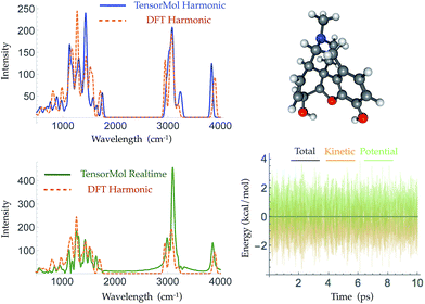
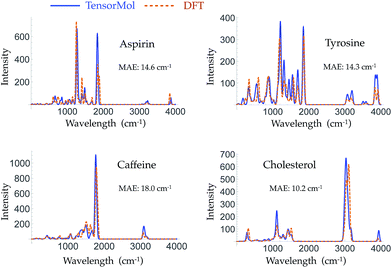
Morphine was not included in our training set. The top right panel of Fig. 7 shows the geometry of morphine that is optimized with our force field. The RMSE of the bond lengths predicted by our force field is 0.0067 Å and the RMSE of the angles is 1.04 degrees, compared with the source DFT model chemistry. The upper left panel plots the harmonic IR spectra generated using DFT and the TensorMol force field, at their respective optimized geometries. One can see the IR spectrum generated using our force field is in good agreement with the DFT-generated IR spectrum. The MAE in our force field frequencies is 13.7 cm⁻¹ compared with the DFT frequencies, which is about half of the MAE in the prediction using MMFF94⁹⁹ (Fig. S3†). Fig. 8 shows comparisons of the IR spectra that are generated using these two methods for aspirin, typrosine, caffeine and cholesterol. All four of these molecules were not included in the training set. The MAE in the frequencies predicted by our field is less than 20 cm⁻¹ for all four molecules, compared with the target DFT frequencies. As Fig. S4† shows, the MAE in the frequencies calculated using MMFF94 are 2 to 3 times larger than the MAE in the frequencies calculated using our force field for these four molecules. The intensities calculated using MMFF94 are also qualitatively different to the DFT intensities. The concept of a chemical bond and force constant are not enforced in any way, yet good agreement with DFT is obtained at a tiny fraction of the original cost.

Fig. 7 The geometry of morphine as optimized by TensorMol-0.1 (upper right panel) and its harmonic IR spectra simulated using ωB97X-D/6-311G** (dashed orange line) and the TensorMol force field (solid blue line) (upper left panel). The lower panels show the real-time IR spectra obtained using TensorMol (solid green line), and the DFT results (dashed orange line) (left), and the conservation of energy maintained by the smoothness of the energy (right).

Fig. 8 Harmonic IR spectra of four different molecules simulated using ωB97X-D/6-311G** (dashed orange line) and TensorMol-0.1 (solid blue line). All these molecules were not included in the training set.

Traditional harmonic vibrational spectra require quadratic computational effort, which works against the speed advantage of a NNMC. For large systems, one can use the molecular dynamics functionality of TensorMol to simulate infrared spectra, Fourier transforming the dipole–dipole correlation function of conservative Newtonian dynamics, whose cost grows linearly with the size of the system. The lower left panel of Fig. 7 shows the infrared spectrum produced by propagation in TensorMol-0.1, also showcasing the good energy conservation of TensorMol. Unlike when using a traditional force field, in this case it is non-trivial to obtain smoothly differentiable NNMCs. 64-bit precision needs to be used as the network cannot be made too flexible, and smooth versions of the typical rectified linear units need to be used. Our package can be used in this way to simulate IR spectra of large systems with linear cost.

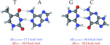
TensorMol-0.1 uses a relatively simple treatment of the electrostatic and van der Waals forces, which we would like to augment in the future with a many-body dispersion scheme.¹⁰⁰ However, a main advantage of the approach used by TensorMol-0.1 is that no self-consistent polarization equation is solved even though the charges are inductive, which results in linear scaling and ease of inexpensively calculating the electrostatic energies of even very large molecules. At shorter ranges, non-covalent interactions like hydrogen bonds are dealt with by the Behler–Parinello portion of the network. The Chemspider training data include some examples of dimers and intra-molecular hydrogen bonds. To our surprise, the treatment of the inter-molecular interactions that were not targets for TensorMol-0.1 are satisfactory. Fig. 9 shows the optimized geometries and binding energies of two DNA base pairs calculated using our force field. The target DFT method predicts a binding energy of 18.3 kcal mol⁻¹ for the thymine–adenine (TA) pair and a binding energy of 32.4 kcal mol⁻¹ for the guanine–cytosine (GC) pair. The prediction using our force field is 1.2 kcal mol⁻¹ smaller for the TA pair and 2.0 kcal mol⁻¹ larger for the GC pair relative to DFT.

Fig. 9 The binding energy between DNA base pairs at their optimized geometries, calculated using DFT (ωB97x-D) and TensorMol methods. The difference between the binding energies calculated using DFT and TensorMol is <2 kcal mol⁻¹.

One holy grail in the field of neural network model chemistries is to simulate biological chemistry without QM-MM or bespoke force fields. Protein simulation also demonstrates several important features of neural network model chemistry: reasonable inter-molecular forces, stability, scalability and generalization far from small-molecule training data. TensorMol-0.1 was not trained on any peptide polymers and includes no biological data of any sort. To our pleasant surprise, even this first iteration of neural network model chemistry is accurate enough to perform rudimentary studies on small proteins. Fig. 10 shows geometries sampled from a 1 picosecond, periodic, 300 K TensorMol dynamics NVT trajectory in explicit solvent. The initial structure (included in the supplementary information) was generated from the PDB structure 2MZX using OpenMM’s automatic solvation and hydrogenation scripts,¹⁰¹ but includes nothing but atom coordinates. This short alpha-helix is stable, both in optimizations and dynamics, and the structures sampled during the dynamics simulation superficially resemble the solution NMR structure. Traditional force fields will always be less expensive (by some prefactor) than NNMCs, yet the reactivity advantages of NNMCs and the ease of set up will probably lead to a rapid adoption of these methods in the biological community.

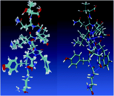Fig. 10 The left panel shows samples from a 1 picosecond NVT (Nosé) trajectory of solvated 2MZX at 300 K, simulated by our TensorMol force field in explicit water. The right panel is the NMR structure of 2MZX from the PDB database.

4 Discussion and conclusions

We have presented a transferable neural network model chemistry, TensorMol-0.1, with long-range coulombic physics and a short-range n-body potential. The model is integrated in an open-source Python package, which provides many of the types of simulation commonly used in chemistry. The method can be used to scan conformational and chemical space along the singlet neutral potential energy surface with high throughput using bare atomic coordinates.

TensorMol-0.1 is not the final iteration of a neural network model chemistry, although it shows that DFT-quality predictions can be made by models with five orders of magnitude lower cost. Inexpensive post-DFT corrections such as many-body dispersion¹⁰⁰ will become even more powerful when integrated with these potentials, opening the door to quantitative treatments of large systems. NNMCs may compete strongly with DFT packages, and provide an interesting complement to QM-MM-type simulations in the near future.

There are several clear paths to extend this work:

• generalize the descriptors to encode other physical atom properties besides charge (spin or polarizability)

• develop accurate descriptors whose cost grows linearly with the number of elements treated

• extend the range of the n-body embedding

• explore the hierarchy of physical detail between force fields and semi-empirical electronic structures

These are the directions of continuing study in our group and others.

Conflicts of interest

There are no conflicts to declare.

References

1. A. Lopez-Bezanilla and O. A. von Lilienfeld, Phys. Rev. B, 2014, 89, 235411.
2. G. Pilania, C. Wang, X. Jiang, S. Rajasekaran and R. Ramprasad, Sci. Rep., 2013, 3, 2810.
3. K. Schütt, H. Glawe, F. Brockherde, A. Sanna, K. Müller and E. Gross, Phys. Rev. B, 2014, 89, 205118.
4. A. P. Bartok, M. C. Payne, R. Kondor and G. Csanyi, Phys. Rev. Lett., 2010, 104, 136403.
5. I. Kruglov, O. Sergeev, A. Yanilkin and A. R. Oganov, Sci. Rep., 2017, 7, 8512.
6. G. R. Medders, A. W. Götz, M. A. Morales, P. Bajaj and F. Paesani, J. Chem. Phys., 2015, 143, 104102.
7. G. R. Medders, V. Babin and F. Paesani, J. Chem. Theory Comput., 2013, 9, 1103–1114.
8. S. K. Reddy, S. C. Straight, P. Bajaj, C. Huy Pham, M. Riera, D. R. Moberg, M. A. Morales, C. Knight, A. W. Götz and F. Paesani, J. Chem. Phys., 2016, 145, 194504.
9. M. Riera, N. Mardirossian, P. Bajaj, A. W. Götz and F. Paesani, J. Chem. Phys., 2017, 147, 161715.
10. D. R. Moberg, S. C. Straight, C. Knight and F. Paesani, J. Phys. Chem. Lett., 2017, 8(12), 2579–2583.
11. S. T. John and G. Csanyi, J. Phys. Chem. B, 2017, 121(48), 10934–10949.
12. S. Chmiela, A. Tkatchenko, H. E. Sauceda, I. Poltavsky, K. T. Schütt and K.-R. Müller, Sci. Adv., 2017, 3, e1603015.
13. L. Mones, N. Bernstein and G. Csanyi, J. Chem. Theory Comput., 2016, 12, 5100–5110.
14. K. Yao and J. Parkhill, J. Chem. Theory Comput., 2016, 12, 1139–1147.
15. J. C. Snyder, M. Rupp, K. Hansen, L. Blooston, K.-R. Müller and K. Burke, J. Chem. Phys., 2013, 139, 224104.
16. F. Brockherde, L. Vogt, L. Li, M. E. Tuckerman, K. Burke and K.-R. Müller, Nat. Commun., 2017, 8, 872.
17. J. C. Snyder, M. Rupp, K. Hansen, K.-R. Müller and K. Burke, Phys. Rev. Lett., 2012, 108, 253002.
18. L. Li, J. C. Snyder, I. M. Pelaschier, J. Huang, U.-N. Niranjan, P. Duncan, M. Rupp, K.-R. Müller and K. Burke, Int. J. Quantum Chem., 2016, 116, 819–833.
19. L. Li, T. E. Baker, S. R. White and K. Burke, et al. , Phys. Rev. B, 2016, 94, 245129.
20. K. Vu, J. C. Snyder, L. Li, M. Rupp, B. F. Chen, T. Khelif, K.-R. Müller and K. Burke, Int. J. Quantum Chem., 2015, 115, 1115–1128.
21. R. T. McGibbon, A. G. Taube, A. G. Donchev, K. Siva, F. Hernández, C. Hargus, K.-H. Law, J. L. Klepeis and D. E. Shaw, J. Chem. Phys., 2017, 147, 161725.
22. J. Wu, L. Shen and W. Yang, J. Chem. Phys., 2017, 147, 161732.
23. F. Fracchia, G. Del Frate, G. Mancini, W. Rocchia and V. Barone, J. Chem. Theory Comput., 2018, 14(1), 255–273.
24. Y. Li, H. Li, F. C. Pickard IV, B. Narayanan, F. G. Sen, M. K. Chan, S. K. Sankaranarayanan, B. R. Brooks and B. Roux, J. Chem. Theory Comput., 2017, 13, 4492–4503.
25. M. Rupp, A. Tkatchenko, K.-R. Müller and O. A. Von Lilienfeld, Phys. Rev. Lett., 2012, 108, 058301.
26. K. Hansen, F. Biegler, R. Ramakrishnan, W. Pronobis, O. A. Von Lilienfeld, K.-R. Müller and A. Tkatchenko, J. Phys. Chem. Lett., 2015, 6, 2326–2331.
27. Y. T. Sun, H. Bai, M.-Z. Li and W. Wang, J. Phys. Chem. Lett., 2017, 8, 3434–3439.
28. R. Jinnouchi and R. Asahi, J. Phys. Chem. Lett., 2017, 8, 4279–4283.
29. L. M. Ghiringhelli, J. Vybiral, E. Ahmetcik, R. Ouyang, S. V. Levchenko, C. Draxl and M. Scheffler, New J. Phys., 2017, 19, 023017.
30. R. Ouyang, S. Curtarolo, E. Ahmetcik, M. Scheffler and L. M. Ghiringhelli, arXiv preprint arXiv:1710.03319, 2017.
31. O. Isayev, C. Oses, C. Toher, E. Gossett, S. Curtarolo and A. Tropsha, Nat. Commun., 2017, 8, 15679.
32. A. Grisafi, D. M. Wilkins, G. Csanyi and M. Ceriotti, arXiv preprint arXiv:1709.06757, 2017.
33. E. Kim, K. Huang, A. Tomala, S. Matthews, E. Strubell, A. Saunders, A. McCallum and E. Olivetti, Sci. Data, 2017, 4, 170127.
34. J. Hachmann, R. Olivares-Amaya, S. Atahan-Evrenk, C. Amador-Bedolla, R. S. Sánchez-Carrera, A. Gold-Parker, L. Vogt, A. M. Brockway and A. Aspuru-Guzik, J. Phys. Chem. Lett., 2011, 2, 2241–2251.
35. J. Hachmann, R. Olivares-Amaya, A. Jinich, A. L. Appleton, M. A. Blood-Forsythe, L. R. Seress, C. Roman-Salgado, K. Trepte, S. Atahan-Evrenk and S. Er, Energy Environ. Sci., 2014, 7, 698–704.
36. O. Isayev, D. Fourches, E. N. Muratov, C. Oses, K. Rasch, A. Tropsha and S. Curtarolo, Chem. Mater., 2015, 27, 735–743.
37. R. Olivares-Amaya, C. Amador-Bedolla, J. Hachmann, S. Atahan-Evrenk, R. S. Sánchez-Carrera, L. Vogt and A. Aspuru-Guzik, Energy Environ. Sci., 2011, 4, 4849–4861.
38. Z. W. Ulissi, M. T. Tang, J. Xiao, X. Liu, D. A. Torelli, M. Karamad, K. Cummins, C. Hahn, N. S. Lewis and T. F. Jaramillo, et al. , ACS Catal., 2017, 7, 6600–6608.
39. C. M. Handley and P. L. Popelier, J. Phys. Chem. A, 2010, 114, 3371–3383.
40. J.-P. Piquemal and K. D. Jordan, J. Chem. Phys., 2017, 147, 161401.
41. K. Mills, M. Spanner and I. Tamblyn, Phys. Rev.A, 2017, 96, 042113.
42. M. Malshe, L. Raff, M. Hagan, S. Bukkapatnam and R. Komanduri, J. Chem. Phys., 2010, 132, 204103.
43. A. A. Peterson, J. Chem. Phys., 2016, 145, 074106.
44. E. D. Cubuk, B. D. Malone, B. Onat, A. Waterland and E. Kaxiras, J. Chem. Phys., 2017, 147, 024104.
45. B. K. Carpenter, G. S. Ezra, S. C. Farantos, Z. C. Kramer and S. Wiggins, J. Phys. Chem. B, 2017 DOI:10.1021/acs.jpcb.7b08707.
46. J. Behler and M. Parrinello, Phys. Rev. Lett., 2007, 98, 146401.
47. J. Behler, Phys. Chem. Chem. Phys., 2011, 13, 17930–17955.
48. K. Shakouri, J. Behler, J. Meyer and G.-J. Kroes, J. Phys. Chem. Lett., 2017, 8, 2131–2136.
49. J. Behler, Angew. Chem., Int. Ed., 2017, 56, 12828–12840.
50. J. Han, L. Zhang, R. Car and W. E, Comm Comput Phys, 2018, 23, 629–639.
51. R. Z. Khaliullin, H. Eshet, T. D. Kühne, J. Behler and M. Parrinello, Nat. Mater., 2011, 10, 693–697.
52. M. Gastegger, J. Behler and P. Marquetand, Chem. Sci., 2017, 8, 6924–6935.
53. R. Kobayashi, D. Giofré, T. Junge, M. Ceriotti and W. A. Curtin, Phys. Rev. B: Condens. Matter Mater. Phys., 2017, 1, 053604.
54. K. Yao, J. E. Herr, S. N. Brown and J. Parkhill, J. Phys. Chem. Lett., 2017, 8(12), 2689–2694.
55. B. Kolb, L. C. Lentz and A. M. Kolpak, Sci. Rep., 2017, 7, 1192.
56. N. Lubbers, J. S. Smith and K. Barros, arXiv preprint arXiv:1710.00017, 2017.
57. A. Khorshidi and A. A. Peterson, Comput. Phys. Commun., 2016, 207, 310–324.
58. K. Yao, J. E. Herr and J. Parkhill, J. Chem. Phys., 2017, 146, 014106.
59. S. Manzhos, R. Dawes and T. Carrington, Int. J. Quantum Chem., 2015, 115, 1012–1020.
60. S. Manzhos, K. Yamashita and T. Carrington Jr, Comput. Phys. Commun., 2009, 180, 2002–2012.
61. K. Shao, J. Chen, Z. Zhao and D. H. Zhang, J. Chem. Phys., 2016, 145, 071101.
62. Z. Zhang and D. H. Zhang, J. Chem. Phys., 2014, 141, 144309.
63. J. Li, J. Chen, Z. Zhao, D. Xie, D. H. Zhang and H. Guo, J. Chem. Phys., 2015, 142, 204302.
64. R. Conte, C. Qu and J. M. Bowman, J. Chem. Theory Comput., 2015, 11, 1631–1638.
65. X. Ma, Z. Li, L. E. Achenie and H. Xin, J. Phys. Chem. Lett., 2015, 6, 3528–3533.
66. J. P. Janet and H. J. Kulik, Chem. Sci., 2017, 8, 5137–5152.
67. J. P. Janet and H. J. Kulik, J. Phys. Chem. A, 2017, 121(46), 8939–8954.
68. F. Häse, C. Kreisbeck and A. Aspuru-Guzik, Chem. Sci., 2017, 8, 8419–8426.
69. T. Bereau, R. A. DiStasio Jr, A. Tkatchenko and O. A. von Lilienfeld, arXiv preprint arXiv:1710.05871, 2017.
70. F. A. Faber, L. Hutchison, B. Huang, J. Gilmer, S. S. Schoenholz, G. E. Dahl, O. Vinyals, S. Kearnes, P. F. Riley and O. A. von Lilienfeld, J. Chem. Theory Comput., 2017, 13(11), 5255–5264.
71. K. T. Schütt, F. Arbabzadah, S. Chmiela, K. R. Müller and A. Tkatchenko, Nat. Commun., 2017, 8, 13890.
72. X.-X. Zhou, W.-F. Zeng, H. Chi, C. Luo, C. Liu, J. Zhan, S.-M. He and Z. Zhang, Anal. Chem., 2017, 89(23), 12690–12697.
73. J. Timoshenko, D. Lu, Y. Lin and A. I. Frenkel, J. Phys. Chem. Lett., 2017, 8(20), 5091–5098.
74. J. Li, D. Cai and X. He, arXiv preprint arXiv:1709.03741, 2017.
75. B. Ramsundar, B. Liu, Z. Wu, A. Verras, M. Tudor, R. P. Sheridan and V. Pande, J. Chem. Inf. Model., 2017, 57, 2068–2076.
76. M. Segler, M. Preuß and M. P. Waller, arXiv preprint arXiv:1702.00020, 2017.
77. G. L. Guimaraes, B. Sanchez-Lengeling, P. L. C. Farias and A. Aspuru-Guzik, arXiv preprint arXiv:1705.10843, 2017.
78. J. N. Wei, D. Duvenaud and A. Aspuru-Guzik, ACS Cent. Sci., 2016, 2, 725–732.
79. R. Gómez-Bombarelli, D. Duvenaud, J. M. Hernández-Lobato, J. Aguilera-Iparraguirre, T. D. Hirzel, R. P. Adams and A. Aspuru-Guzik, arXiv preprint arXiv:1610.02415, 2016.
80. S. Grimme, J. Comput. Chem., 2006, 27, 1787–1799.
81. B. T. Thole, Chem. Phys., 1981, 59, 341–350.
82. J. S. Smith, O. Isayev and A. E. Roitberg, Chem. Sci., 2017, 8, 3192–3203.
83. J. S. Smith, O. Isayev and A. E. Roitberg, Sci. Data, 2017, 4, 170193.
84. J.-D. Chai and M. Head-Gordon, Phys. Chem. Chem. Phys., 2008, 10, 6615–6620.
85. M. Ceriotti, J. More and D. E. Manolopoulos, Comput. Phys. Commun., 2014, 185, 1019–1026.
86. V. L. Deringer and G. Csanyi, Phys. Rev. B, 2017, 95, 094203.
87. T. Morawietz and J. Behler, J. Phys. Chem. A, 2013, 117, 7356–7366.
88. M. Abadi, A. Agarwal, P. Barham, E. Brevdo, Z. Chen, C. Citro, G. S. Corrado, A. Davis, J. Dean, M. Devin, S. Ghemawat, I. Goodfellow, A. Harp, G. Irving, M. Isard, Y. Jia, R. Jozefowicz, L. Kaiser, M. Kudlur, J. Levenberg, D. Mané, R. Monga, S. Moore, D. Murray, C. Olah, M. Schuster, J. Shlens, B. Steiner, I. Sutskever, K. Talwar, P. Tucker, V. Vanhoucke, V. Vasudevan, F. Viégas, O. Vinyals, P. Warden, M. Wattenberg, M. Wicke, Y. Yu and X. Zheng, TensorFlow: Large-Scale Machine Learning on Heterogeneous Systems, 2015, http://tensorflow.org/.
89. C. J. Fennell and J. D. Gezelter, J. Chem. Phys., 2006, 124, 234104.
90. T. Morawietz, V. Sharma and J. Behler, J. Chem. Phys., 2012, 136, 064103.
91. N. Artrith, T. Morawietz and J. Behler, Phys. Rev. B, 2011, 83, 153101.
92. D.-A. Clevert, T. Unterthiner and S. Hochreiter, arXiv preprint arXiv:1511.07289, 2015.
93. J. E. Herr, K. Yao, R. McIntyre, D. Toth and J. Parkhill, arXiv preprint arXiv:1712.07240, 2017.
94. Y. Shao, Z. Gan, E. Epifanovsky, A. T. Gilbert, M. Wormit, J. Kussmann, A. W. Lange, A. Behn, J. Deng and X. Feng, et al. , Mol. Phys., 2015, 113, 184–215.
95. N. Srivastava, G. E. Hinton, A. Krizhevsky, I. Sutskever and R. Salakhutdinov, J. Mach. Learn. Res., 2014, 15, 1929–1958.
96. D. Kingma and J. Ba, arXiv preprint arXiv:1412.6980, 2014.
97. G. Henkelman, B. P. Uberuaga and H. Jónsson, J. Chem. Phys., 2000, 113, 9901–9904.
98. A. Barducci, G. Bussi and M. Parrinello, Phys. Rev. Lett., 2008, 100, 020603.
99. T. A. Halgren, J. Comput. Chem., 1996, 17, 553–586.
100. A. Tkatchenko, R. A. DiStasio Jr, R. Car and M. Scheffler, Phys. Rev. Lett., 2012, 108, 236402.
101. P. Eastman, J. Swails, J. D. Chodera, R. T. McGibbon, Y. Zhao, K. A. Beauchamp, L.-P. Wang, A. C. Simmonett, M. P. Harrigan, C. D. Stern, R. P. Wiewiora, B. R. Brooks and V. S. Pande, PLoS Comput. Biol., 2017, 13, 1–17.

---

Footnote

† Electronic supplementary information (ESI) available. See DOI: 10.1039/c7sc04934j

---