Experimental design and machine learning strategies for parameters screening and optimization of Hantzsch condensation reaction for the assay of sodium alendronate in oral solution
Mohamed A. Koranya,
Marwa A. A. Ragab*a,
Rasha M. Youssefa and
Mostafa A. Afifyb
aFaculty of Pharmacy, Department of Pharmaceutical Analytical Chemistry, University of Alexandria, El-Messalah, Alexandria 21521, Egypt. E-mail: marmed_2001@yahoo.com; Fax: +20 3 4873273; Tel: +20 3 4871317
bBorg Pharmaceutical Industries, Borg El-Arab new city – Industrial Zone 3 – Area 3 – district 17, Alexandria, Egypt
First published on 4th December 2014
Abstract
An experimental design was adopted to attain the optimum reaction parameters of chemical derivatization of anhydrous sodium alendronate in an oral solution formula via Hantzsch condensation reaction. All reaction controlling variables, namely, time of reaction, temperature, reagent ratio and volume and buffer type, pH and volume were studied using the Plackett–Burman screening design to determine significant variables. Reaction temperature and pH of the buffer solution were found to be significant variables. Optimization was performed using the central composite design to get the optimum levels of these variables. Moreover, a comparison was made with artificial neural networks and support vector machines. The same results were obtained with low percentage relative error. After carrying out the spectrophotometric analysis, interferences from oral solution excipients were eliminated with a simple extraction procedure before measuring the absorbance at 340 nm. Satisfactory results of sample analysis were obtained and they were in good agreement with the label claim. A linear calibration graph of absorbance versus concentration was obtained with very low value of intercept and high value of correlation coefficient (0.9999) in the range of 2.44–34.10 μg mL−1. The proposed spectrophotometric method was fully validated in accordance with ICH guidelines. Statistical comparison with a reported reference method showed similar results with respect to accuracy and precision.
1. Introduction
Anhydrous sodium alendronate (ALN); (4-amino-1-hydroxybutylidene) diphosphonic acid mono sodium salt; (Fig. 1) is an aminobisphosphonate with general properties similar to those of the other bisphosphonates.1,2 It is a potent inhibitor of bone resorption and is given for the management of osteoporosis either alone or with vitamin D. ALN is used for the treatment of Paget's disease of bone. It has also been given in the treatment of bone metastases and hypercalcaemia of malignancy. ALN tablet formulation has a precaution that patients should swallow entire tablets with plenty of water. Thus, a single dose 75 mL of ALN oral solution was formulated.1,2 ALN structure lacks any chromophore, and hence it cannot be determined by direct spectrophotometric methods. ALN is official in the USP 36 and BP 2013. The official methods reported for ALN assay exhibit some difficulties and need sophisticated instruments.2,3 For the USP method of ALN assay in tablets, the reagent used for precolumn derivatization is very toxic and carcinogenic, 9-fluorenylmethyl chloroformate. Furthermore, separation from excess reagent is needed by carrying out an extraction step using methylene chloride. Next, chromatographic separation was conducted using the styrene–DVB polymer column with UV detection.2 The BP method depends on direct assay using ion exchange chromatography, which is known to be time consuming as the equilibration of the column takes a long time, and inverse UV detection.3Therefore, several methods were reported for ALN assay. Spectrophotometric methods were reported for the assay of ALN.4–14 However, the proposed method has limits of detection and quantitation that are considerably lower than those of many other published methods.5–7,12,13 Moreover, some of the mentioned spectrophotometric methods have a narrow linear dynamic range when compared to the proposed method.4,13,14 In addition, spectrophotometric methods depending on the reaction of the amino group of ALN with ninhydrin reagent are non-specific as only the amino group moiety of the drug will be contained in the reaction product without the rest of the molecule, thus the colored derivative is the same irrespective of the primary amine precursor.11,13 Moreover, HPLC methods were described for its analysis.2,3,6,15 ALN was electrochemically16 determined. A fluorimetric method was reported for the quantification of alendronate and clodronate in aqueous samples and in serum.17 Some capillary electrophoresis methods were described for the determination of ALN.18 A literature review reports some methods for the determination of ALN in tablets5,6,19–21 but it lacks any reported method for the assay of ALN in oral solution.
The Hantzsch condensation reaction depends on the formation of dihydrolutidine derivatives when a β-dicarbonyl compound condenses with an aldehyde and a primary amine or ammonia.22 This reaction is widely used by different analytical techniques, including spectrophotometric, spectrofluorimetric and chromatographic methods.23–27
The Hantzsch condensation reaction is considered to be a perfect example for investigating the effectiveness of the experimental design and machine learning strategies in screening and optimizing the high number of parameters affecting such reaction. These parameters include time of reaction, temperature, reagent ratio and volume and buffer type, pH and volume.
Few examples were found in literature screening and optimization the experimental parameters affecting dispersive liquid–liquid microextraction,28 solid-phase extraction29 and chromatographic separations.30 No literature was found for the investigation of the effectiveness of experimental design31,32 and machine learning strategies in screening and optimizing parameters affecting such reaction.
The different conditions for the optimization of the condensation reaction were studied using the experimental design (DOE) approach in two stages. The first involves screening design, which is Plackett–Burman design (PBD) for variable screening. The second involves the application of circumscribed central composite design (CCCD) for the optimization of significant variables. A comparison was performed among CCCD, artificial neural networks (ANN) and support vector machines (SVM).
The theoretical background of these methods was extensively discussed in literature.33–37 Although the univariate procedures (one variable at a time; OVAT) are time and effort consuming, they are still being used in routine methods. In this work, the multivariate design of experiments (DOE or experimental design) is considered because it takes less time, effort and resources than the OVAT method. DOE and the response surface methodology (RSM) were useful for improving and optimizing processes. The RSM has been widely used in analytical and industrial applications.33
Screening designs are used to specify the most significant factors from those potentially affecting the considered responses. Most often, two-level screening designs, such as fractional factorial or Plackett–Burman designs, are used, which allow examining a relatively high number of factors f at L = 2 levels in a relatively small number of experiments (N ≥ f + 1). When f is small, two-level full factorial designs might also be applied for screening purposes.34
A Plackett–Burman design (PBD) is used here for screening, which allows examining maximally f = N − 1 factors in N experiments, where N is a multiple of four (N = 8, 12, 16, 20, …). When f exceeds the number of real factors to be examined, the remaining columns of the PBD are defined as dummy factor columns.34
A central composite design (CCD) contains a two-level full factorial design (2f experiments), a star design (2f experiments) and a centre point, requiring N = 2f + 2f + 1 experiments to examine f factors. As a result, 9 experiments are needed for two factors, while 15 are needed for three factors. The points of the full factorial design are situated at the factor levels −1 and +1, those of the star design at the factor levels 0, −α and +α (where α is the distance from centre point to star points in CCD (axial distance)), and the centre point at the factor levels 0. Depending on the value, two CCDs exist, i.e. a face-centred CCD (FCCD) with |α| = 1 examining the factors at three levels, and a circumscribed CCD (CCCD) with |α| > 1 examining the factors at five levels. For a so-called rotatable CCCD, the level should be |α| = (2f)1/4, i.e. 1.41 and 1.68 for 2 and 3 factors, respectively (Fig. 2).34,35 A CCCD was used for the optimization of significant factors of this work in 2 blocks. If the number of experiments exceeds the number of experiments that can be performed in one day, the experiments should be performed in blocks.33
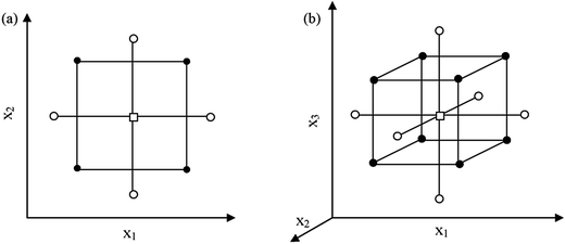 | ||
| Fig. 2 Central composite designs for the optimization of: (a) two variables (α = 1.41) and (b) three variables (α = 1.68). (●) points of factorial design, (○) star points and (□) central point. | ||
The artificial neural networks (ANN) methodology is an information-processing chemometric technique specially created to model non-linear information, which simulates some properties of the human brain. The so called multilayer feed-forward networks, or multi-layer perceptron (MLP) networks, are often used for prediction, as well as for classification.
It is important to stress that ANN have a notable advantage, as there is no need to know the exact form of the analytical function on which the model should be built. Furthermore, neither the functional type nor the number of model parameters need to be given. This is the main difference between modeling by LS regression and ANN.33
In a short period of time, support vector machines (SVM) found many applications in chemistry. For example in drug design, it was used for discriminating between ligands and non-ligands, inhibitors and non-inhibitors. Moreover, in quantitative structure-activity relationships (QSAR), SVM regression is used to predict various physical, chemical, or biological properties. Moreover, SVM was a very useful tool in chemometrics dealing with the optimization of chromatographic separation or compound concentration prediction from spectral data as examples, in sensors (for qualitative and quantitative prediction from sensor data), in chemical engineering (fault detection and modeling of industrial processes) and text mining (automatic recognition of scientific information).37
Support vector machines represent an extension to nonlinear models of the generalized portrait algorithm developed by Vapnik and Lerner. The SVM algorithm is based on the statistical learning theory and the Vapnik–Chervonenkis (VC) dimension. SVM models were originally defined for the classification of linearly separable classes of objects.37 SVR is famous for handling nonlinear data through kernels, however, it can also handle linear data.38
In this work, we use a radial basis function-support vector machines regression (RBF-SVR) model, in which nonlinearity of the used data is the case due to the presence of interactions between the reaction variables.
The aim of this work is to investigate, for the first time, the effectiveness of experimental design and machine learning strategies for screening and optimizing the Hantzsch condensation reaction. This reaction was successfully applied for the indirect spectrophotometric determination of ALN, which contains no chromophore, in oral solution. Hantzsch condensation reaction was a suitable example for investigating the effectiveness of such methods as it is affected by a large number of parameters. Plackett–Burman screening design was used to determine significant variables. After that, optimization was performed using the central composite design to get the optimum levels of these variables. A comparison was performed with artificial neural networks and support vector machines. The same results were obtained with low percentage relative error. Moreover, a full validation of the spectrophotometric method was performed in accordance with ICH guidelines. The optimized method was then applied to the spectrophotometric determination of the drug in oral solutions.
2. Experimental
2.1. Materials and Reagents
Pharmaceutical grade ALN was supplied as a gift sample by Borg Pharmaceutical Industries, Alexandria, Egypt. All the reagents used were of analytical grade. Formaldehyde solution (37% w/w) was purchased from Merck KGaA, Darmstadt, Germany. Sodium hydroxide and glacial acetic acid (Sigma-Aldrich®, St. Louis, MO, United States), methylene chloride (CDH Limited, New Delhi, India) and sodium acetate trihydrate and citric acid monohydrate (Fisher Scientific UK Ltd, Bishop Meadow Road, Loughborough) were used. The water used was reverse osmosis water. Borgalendro® oral solution (Batch no. 082001) labeled to contain 91.35 mg of anhydrous sodium alendronate (equivalent to 70 mg alendronic acid) per 75 mL unit dose bottle was supplied as a gift sample by Borg Pharmaceutical Industries, Alexandria, Egypt.2.2. Instrumentation
An Agilent UV-vis Spectrophotometer model no: 8453, equipped with 1 cm quartz cell and running with ChemStation software (Germany), a Sartorius balance TE 214S, Sartorius (Germany), a Jenway pH meter equipped with a glass combination electrode (UK), an Elma ultrasonic sonicator, model: Elmasonic S 120. (Singen/Hohentwiel, Germany) and a Memmert GmbH & Co. KG water bath type WNB 22 (Germany) were used throughout the work.2.3. Preparation of reagents
2.4. Stock solutions
Stock solution of 6.09 mg mL−1 of ALN was prepared in purified water and further diluted with the same solvent to obtain different working standard solutions of suitable concentrations (121.8, 243.6, 974.4, 1218.0 and 1705.2 μg mL−1).2.5. Construction of calibration graph
To prepare different final standard solutions in the linearity range, a volume of 1 mL from each working standard solution is quantitatively transferred into a series of test tubes and a blank was prepared using 1 mL water instead of drug working standard solutions. Then, 3 mL reagent was added to each test tube and these test tubes were placed in a boiling water bath for 15 minutes. Next, the test tubes were cooled and their contents were quantitatively transferred into 50 mL volumetric flasks and the volume was completed to mark using purified water. From each volumetric flask, a volume of 10 mL was transferred into a series of centrifuge tubes containing 20 mL methylene chloride. The centrifuge tubes were shaken for 1 minute, sonicated for 30 minutes and allowed to cool for 15 minutes. The absorbance of the aqueous layer of each final standard solution (2.44, 4.87, 19.49, 24.36 and 34.10 μg mL−1) was measured against blank in a 1 cm cell at 340 nm.2.6. Preparation of oral solution
One mL oral solution was quantitatively transferred into a test tube and the procedure was completed on the prepared solution as under Construction of calibration graph section in order to obtain a final dilution of 24.36 μg mL−1.3. Results and discussion
3.1. Condensation reaction
Based on the Hantzsch condensation reaction, ALN reacts with a β-dicarbonyl compound (acetylacetone) and an aldehyde (formaldehyde) to produce a yellow colored product, which was measured spectrophotometrically at λ = 340 nm. The reaction mechanism of ALN with acetylacetone and formaldehyde is proposed in Fig. 3.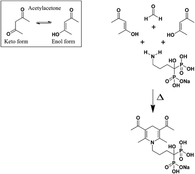 | ||
| Fig. 3 A proposed reaction mechanism for Hantzsch condensation reaction of ALN with acetylacetone and formaldehyde. | ||
3.2. Selection of variables and screening of significant variables
Variables that may affect the condensation reaction, illustrated in Table 1, were selected for PBD for screening. Four central points were added for error estimation.33 The design was generated using StatSoft STATISTICA 10 software.| Trial no. | t (min) | T (°C) | RR (A![[thin space (1/6-em)]](https://www.rsc.org/images/entities/char_2009.gif) : :![[thin space (1/6-em)]](https://www.rsc.org/images/entities/char_2009.gif) F)c F)c |
RV (mL) | pH | BTd | BV (mL) | Maximum absorbancee |
|---|---|---|---|---|---|---|---|---|
| a t is the reaction time, T is the reaction temperature, RR is the reagent ratio, RV is the reagent volume, pH is the pH of the buffer used, BT is the buffer type, and BV is the buffer volume.b “(C)” denotes center points.c “A” stands for acetylacetone while “F” stands for 37% w/w formaldehyde solution. 0.5: 2.0 mL of A + 4.0 mL of F + 4.0 mL of water. 2: 4.0 mL of A + 2.0 mL of F + 4.0 mL of water. 1.25: 2.5 mL of A + 2.0 mL of F + 3.0 mL of water.d Both buffer types are of 0.1 M strength.e Ranging from λ = 330–340 nm. | ||||||||
| 1 | 15.00 (−1) | 21.50 (−1) | 0.50 (−1) | 1.00 (1) | 5.80 (1) | Acetate (1) | 0.50 (−1) | 0.12941 |
| 2 | 15.00 (−1) | 21.50 (−1) | 2.00 (1) | 1.00 (1) | 3.80 (−1) | Citrate (−1) | 2.00 (1) | 0.01378 |
| 3 | 15.00 (−1) | 95.00 (1) | 0.50 (−1) | 0.25 (−1) | 5.80 (1) | Citrate (−1) | 2.00 (1) | 0.28700 |
| 4 | 15.00 (−1) | 95.00 (1) | 2.00 (1) | 0.25 (−1) | 3.80 (−1) | Acetate (1) | 0.50 (−1) | 0.47332 |
| 5 | 60.00 (1) | 21.50 (−1) | 0.50 (−1) | 0.25 (−1) | 3.80 (−1) | Acetate (1) | 2.00 (1) | 0.13053 |
| 6 | 60.00 (1) | 21.50 (−1) | 2.00 (1) | 0.25 (−1) | 5.80 (1) | Citrate (−1) | 0.50 (−1) | 0.0104 |
| 7 | 60.00 (1) | 95.00 (1) | 0.50 (−1) | 1.00 (1) | 3.80 (−1) | Citrate (−1) | 0.50 (−1) | 0.36474 |
| 8 | 60.00 (1) | 95.00 (1) | 2.00 (1) | 1.00 (1) | 5.80 (1) | Acetate (1) | 2.00 (1) | 0.52309 |
| 9 (C)b | 37.50 (0) | 58.25 (0) | 1.25 (0) | 0.63 (0) | 4.80 (0) | Citrate (−1) | 1.25 (0) | 0.19312 |
| 10 (C)b | 37.50 (0) | 58.25 (0) | 1.25 (0) | 0.63 (0) | 4.80 (0) | Acetate (1) | 1.25 (0) | 0.19876 |
| 11 (C)b | 37.50 (0) | 58.25 (0) | 1.25 (0) | 0.63 (0) | 4.80 (0) | Citrate (−1) | 1.25 (0) | 0.19791 |
| 12 (C)b | 37.50 (0) | 58.25 (0) | 1.25 (0) | 0.63 (0) | 4.80 (0) | Acetate (1) | 1.25 (0) | 0.19711 |
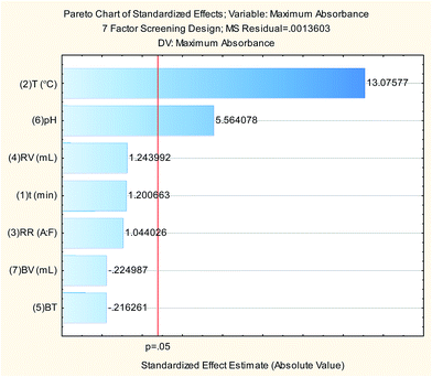
The 7-factors 4-center points PBD trials shown in Table 1 were performed using 1 mL working standard solution (to give final standard solution of a concentration of 24.36 μg mL−1). For each trial, standard was measured spectrophotometrically against the corresponding blank and the maximum absorbance was recorded and entered in the design matrix using StatSoft STATISTICA 10 software for subsequent data analysis. Results are illustrated in Table 1 and Pareto chart (Fig. 4) shows that reaction temperature and pH of the buffer are the only significant factors at p-value = 0.05. ANOVA analysis (Table 2) shows good agreement with the experimental data (high values of R2 and adjusted R2).
| Factor | SS | df | MS | F | p |
|---|---|---|---|---|---|
| a t is the reaction time, T is the reaction temperature, RR is the reagent ratio, RV is the reagent volume, pH is the pH of the buffer used, BT is the buffer type, BV is the buffer volume, SS is sum of squares, df is degrees of freedom and MS is mean of squares. Significant factors (p-value = 0.05) appear in bold.b “A” stands for acetylacetone while “F” stands for 37% (w/w) formaldehyde solution. | |||||
| (1) t (min) | 0.001961 | 1 | 0.001961 | 1.4416 | 0.296121 |
| (2) T (°C) | 0.232572 | 1 | 0.232572 | 170.9758 | 0.000197 |
(3) RR (A![[thin space (1/6-em)]](https://www.rsc.org/images/entities/char_2009.gif) : :![[thin space (1/6-em)]](https://www.rsc.org/images/entities/char_2009.gif) F)b F)b |
0.001483 | 1 | 0.001483 | 1.0900 | 0.355413 |
| (4) RV (mL) | 0.002105 | 1 | 0.002105 | 1.5475 | 0.281422 |
| (5) BT | 0.000064 | 1 | 0.000064 | 0.0468 | 0.839365 |
| (6) pH | 0.042112 | 1 | 0.042112 | 30.9590 | 0.005110 |
| (7) BV (mL) | 0.000069 | 1 | 0.000069 | 0.0506 | 0.833016 |
| Error | 0.005441 | 4 | 0.001360 | ||
| Total SS | 0.285807 | 11 | |||
| R2 | 0.98096 | ||||
| Adjusted R2 | 0.94765 | ||||
3.3. Optimization of the reaction variables
| Trial no. | Block | T (°C) | pH | Absorbancec |
|---|---|---|---|---|
| a T is the reaction temperature and pH is the pH of the acetate buffer.b “(C)” denotes center points.c At λ = 340 nm. | ||||
| 1 | 1 | 75.00 (−1.00) | 3.50 (−1.00) | 0.08952 |
| 2 | 1 | 75.00 (−1.00) | 6.50 (1.00) | 0.25332 |
| 3 | 1 | 95.00 (1.00) | 3.50 (−1.00) | 0.35412 |
| 4 | 1 | 95.00 (1.00) | 6.50 (1.00) | 0.32158 |
| 5 (C)b | 1 | 85.00 (0.00) | 5.00 (0.00) | 0.39515 |
| 6 | 2 | 70.86 (−1.41) | 5.00 (0.00) | 0.29174 |
| 7 | 2 | 99.14 (1.41) | 5.00 (0.00) | 0.51417 |
| 8 | 2 | 85.00 (0.00) | 2.88 (−1.41) | 0.14871 |
| 9 | 2 | 85.00 (0.00) | 7.12 (1.41) | 0.32323 |
| 10 (C)b | 2 | 85.00 (0.00) | 5.00 (0.00) | 0.40513 |
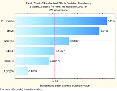
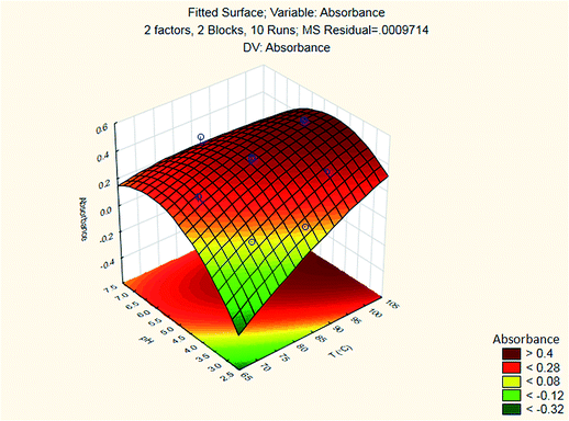
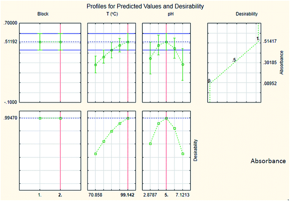
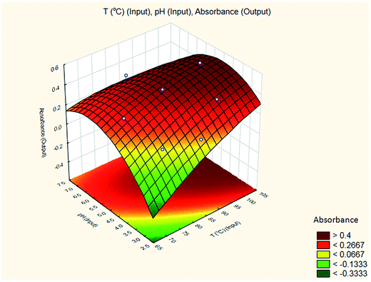
The results are shown in Table 3 and the subsequent statistical analysis using StatSoft STATISTICA 10 software is shown in the Pareto chart (Fig. 5), the ANOVA table (Table 4) shows good agreement with the experimental data (high values of R2 and adjusted R2), and a response surface plot (Fig. 6) shows the relation between the two significant variables to be optimized and absorbance. It was found that for these variables, the temperature relation with absorbance was linear more than quadratic, whereas the relation of the buffer solution pH with absorbance was both linear and quadratic (Fig. 5, 7 and Table 4). The desirability function graph (Fig. 7) shows the optimum levels for both reaction temperature (99.14 °C) and pH of the buffer solution (5.0).
| Percentage relative error (Er%) of predicted optimum and observed optimum = −0.44%. |
| Factor | SS | df | MS | F | p |
|---|---|---|---|---|---|
| a T is the reaction temperature, pH is the pH of the acetate buffer, L is linear effect, Q is quadratic effect, SS is sum of squares, df is degrees of freedom and MS is mean of squares. Significant factors (p-value = 0.05) appear in bold. | |||||
| Blocks | 0.007251 | 1 | 0.007251 | 7.46478 | 0.071809 |
| (1) T (°C) (L) | 0.052394 | 1 | 0.052394 | 53.93539 | 0.005217 |
| T (°C) (Q) | 0.001001 | 1 | 0.001001 | 1.03083 | 0.384725 |
| (2) pH (L) | 0.017868 | 1 | 0.017868 | 18.39382 | 0.023301 |
| pH (Q) | 0.044166 | 1 | 0.044166 | 45.46537 | 0.006662 |
| 1L by 2L | 0.009638 | 1 | 0.009638 | 9.92103 | 0.051275 |
| Error | 0.002914 | 3 | 0.000971 | ||
| Total SS | 0.138413 | 9 | |||
| R2 | 0.97895 | ||||
| Adjusted R2 | 0.93684 | ||||
The predictive equation is:
| z = −3.9974861300552 + 0.049615109658483x − 0.0001480033125x2 + 0.746510940046y − 0.043685358333334y2 − 0.0032723600000001xy + 0. |
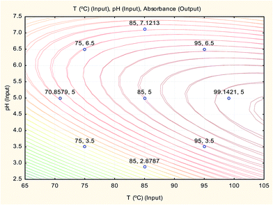
A suitable method to find the optimal location is through the graphical representation of the model. Two types of graphs may provide helpful results: (a) the response surface in the three dimensional space and (b) the graph of contours that is the projection of the surface in a plane, represented as lines of constant response. Each contour corresponds to a specific height of the surface.33 Hence, a surface plot between independent variables (reaction temperature and pH of the buffer solution) and dependent variable (absorbance) was plotted and carefully examined as illustrated in Fig. 8.
| Percentage relative error (Er%) of predicted optimum and observed optimum = −0.007%. |
The overlay contour plot of both CCCD and ANN predictive models (Fig. 9) shows coincidence of the optimal location for both optimization techniques at the maximum temperature of the water bath and the pH of the buffer solution equal to 5.0.
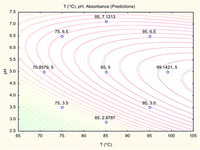
In a similar manner to ANN, optimal location was determined by plotting and carefully examining the surface plot.
| Percentage relative error (Er%) of predicted optimum and observed optimum = −0.41%. |
The overlay contour plot of both CCCD and SVM predictive models (Fig. 10) shows coincidence of the optimal location for both optimization techniques at the maximum temperature of the water bath and the pH of the buffer solution equal to 5.0.
Therefore, the three optimisation techniques (CCCD, ANN and SVM) gave the same results with a low value of error percent (Er%), which confirms that pH 5.0 for the buffer solution and a boiling water bath are the optimum conditions for Hantzsch condensation reaction of sodium alendronate for its determination in oral solution formula.
3.4. Optimization of extraction procedure
On application of the proposed method without an extraction step on the oral solution formula, a recovery above 115% was obtained. Thus, a further investigation was done by applying the procedure on a placebo preparation that shows recovery above 15%. Thus, the extraction step was carried out using another organic solvent that is immiscible with water as the resulting derivative has a highly polar moiety in its chemical structure coming from ALN as illustrated in Fig. 3. Other suspected interferents are known to be less polar, which are most probably methylparaben and propylparaben. Each inactive ingredient in the dosage form other than methylparaben and propylparaben (citric acid, sodium citrate, raspberry flavor and sucralose), was allowed to undergo the procedure (either alone or spiked with ALN) without the extraction step and obtained accurate results in the ALN assay. Organic solvents heavier than water were preferred to avoid the use of separating funnels that make the procedure more time and effort consuming. Hence, methylene chloride was tried by adding 20 mL into a centrifuge tube containing 10 mL of the derivatised solutions with vigorous shaking for 1 minute. Sonication was performed for 30 minutes to break down the formed emulsion, and then the solutions were allowed to cool for 15 minutes. Upon measurement of the solution, accurate results were obtained. Shaking for less than 1 minute led to inaccurate results. Sonication less than 30 minutes was insufficient for breaking the emulsion.3.5. Validation
Using the optimized reaction parameters, the developed spectrophotometric method was validated in terms of linearity, accuracy and precision.![[thin space (1/6-em)]](https://www.rsc.org/images/entities/char_2009.gif) 459.47191), indicate good linearity of the calibration graph.
459.47191), indicate good linearity of the calibration graph.| Concentration (μg mL−1) | Mean % recovery ± SD | RSD (%) | Er (%) |
|---|---|---|---|
| a Mean ± standard deviation of three determinations. | |||
| (a) Intra-day precision and accuracy | |||
| 0.00 (placebo) | 0.68 ± 3.79 × 10⁻² | 5.56 | 0.68 |
| 19.47 | 100.73 ± 1.65 × 10⁻¹ | 0.20 | 0.73 |
| 24.34 | 98.47 ± 9.62 × 10⁻² | 0.10 | −1.53 |
| 29.21 | 100.31 ± 3.32 × 10⁻¹ | 0.28 | 0.31 |
| (b) Inter-day precision and accuracy | |||
| 0.00 (placebo) | −0.41 ± 2.27 × 10⁻¹ | −55.90 | −0.41 |
| 19.47 | 98.52 ± 2.60 × 10⁻¹ | 0.33 | −1.48 |
| 24.34 | 99.37 ± 2.61 × 10⁻¹ | 0.26 | −0.63 |
| 29.21 | 98.63 ± 2.12 × 100 | 1.79 | −1.37 |
4. Conclusion
Experimental design and machine learning strategies were investigated and compared for the parameter screening and optimization of the Hantzsch condensation reaction for ALN in its oral solution. PBD was used for screening of the reaction parameters, whereas the optimization was performed using CCCD, ANN and SVM. The three optimization techniques gave the same results with low Er%. After method optimization, ALN was assayed using the proposed spectrophotometric method, which was fully validated. Interferences from oral solution excipients were eliminated with a simple extraction procedure before measuring the absorbance at 340 nm. Although the Hantzsch condensation reaction is affected by a large number of parameters to be optimized, the experimental design and machine learning strategies used allow fast and accurate optimization of these parameters. Thus, spectrophotometric reactions, which are affected by too many factors can be simply applied by the aid of smart chemometric techniques.References
- S. C. Sweetman, Martindale: The Complete Drug Reference, Pharmaceutical Press, 2011 Search PubMed.
- U. S. P. Convention, USP36 NF31, 2013: U. S. Pharmacopoeia National Formulary, United States Pharmacopeial, 2012 Search PubMed.
- U. K. S. Office, British Pharmacopoeia 2013 [Print + CD-ROM], STATIONARY OFFICE, 2012 Search PubMed.
- A. Raza and M. Zia-Ul-Haq, Int. J. Anal. Chem., 2011, 680902(6) Search PubMed.
- M. I. Walash, M. E. Metwally, M. Eid and R. N. El-Shaheny, Chem. Cent. J., 2012, 6, 25 CrossRef CAS PubMed.
- S. K. Al Deeb, I. I. Hamdan and S. M. Al Najjar, Talanta, 2004, 64, 695–702 CrossRef CAS PubMed.
- S. Panda, B. Ravikumar and D. Patanaik, Int. J. Pharm. Sci. Nanotechnol., 2012, 4, 1563–1568 Search PubMed.
- M.-l. LONG, H.-l. HUANG and Y.-q. SHENG, J. Nanhua Univ., Med. Ed., 2007, 1, 032 Search PubMed.
- M. Long, H. Huang and F. Yan, Chin. Pharm. J., 2006, 22, 434–436 CAS.
- J. Kuljanin, I. Jankovic, J. Nedeljkovic, D. Prstojevic and V. Marinkovic, J. Pharm. Biomed. Anal., 2002, 28, 1215–1220 CrossRef CAS.
- N. A. Alarfaj, S. A. Abd El-Razeq and F. N. Al-Qahtani, Asian J. Chem., 2011, 23, 697–700 CAS.
- M. Koba, K. Koba and L. Przyborowski, Acta Pol. Pharm., 2008, 65, 289–294 CAS.
- E. A. Taha and N. F. Youssef, Chem. Pharm. Bull., 2003, 51, 1444–1447 CrossRef CAS.
- C. Yan-Ping and L. Ming-Li, Pharm. J. Chin. People's Liberation Army, 2008, 171–173 Search PubMed.
- J. Meng, Q. Meng and L. Zheng, Biomed. Chromatogr., 2010, 24, 169–173 CAS.
- O. A. Razak, S. F. Belal, M. M. Bedair and R. S. Haggag, Talanta, 2003, 59, 1061–1069 CrossRef CAS.
- W. Ulbrich and A. Lamprecht, Talanta, 2011, 84, 437–442 CrossRef CAS PubMed.
- S. W. Su, Y. C. Liao and C. W. Whang, J. Sep. Sci., 2012, 35, 681–687 CrossRef CAS PubMed.
- B. Xie, A. Liu, X. Fang, Y. Chen and H. Zhong, J. Pharm. Biomed. Anal., 2014, 93, 73–76 CrossRef CAS PubMed.
- D. G. Reed, G. P. Martin, J. M. Konieczny and M. A. Brooks, J. Pharm. Biomed. Anal., 1995, 13, 1055–1058 CrossRef CAS.
- E. W. Tsai, D. P. Ip and M. A. Brooks, J. Chromatogr., 1992, 596, 217–224 CrossRef CAS.
- S. M. Sabry, M. Abdel-Hady, M. Elsayed, O. T. Fahmy and H. M. Maher, J. Pharm. Biomed. Anal., 2003, 32, 409–423 CrossRef CAS.
- S. Zali, F. Jalali, A. Es-haghi and M. Shamsipur, J. Sep. Sci., 2013, 36, 3883–3888 CrossRef CAS PubMed.
- M. Saenz, J. Alvarado, F. Pena-Pereira, S. Senra-Ferreiro, I. Lavilla and C. Bendicho, Anal. Chim. Acta, 2011, 687, 50–55 CrossRef CAS PubMed.
- H. Bagheri, M. Ghambarian, A. Salemi and A. Es-Haghi, J. Pharm. Biomed. Anal., 2009, 50, 287–292 CrossRef CAS PubMed.
- Q. Li, P. Sritharathikhun and S. Motomizu, Anal. Sci., 2007, 23, 413–417 CrossRef.
- D. L. Cinti and S. E. Thal, Anal. Biochem., 1977, 83, 91–98 CrossRef CAS.
- S. Khodadoust and M. Ghaedi, Spectrochim. Acta, Part A, 2014, 133, 87–92 CrossRef CAS PubMed.
- H. Ebrahimzadeh, N. Tavassoli, O. Sadeghi and M. Amini, Talanta, 2012, 97, 211–217 CrossRef CAS PubMed.
- E. C. Demiralay, Acta Chim. Slov., 2012, 59, 307–314 CAS.
- P. A. Hopes, A. J. Parker and I. Patel, Org. Process Res. Dev., 2006, 10, 808–813 CrossRef CAS.
- B. Norcross, G. Clement and M. Weinstein, J. Chem. Educ., 1969, 46, 694 CrossRef CAS.
- L. Vera Candioti, M. M. De Zan, M. S. Camara and H. C. Goicoechea, Talanta, 2014, 124C, 123–138 CrossRef PubMed.
- B. Dejaegher and Y. V. Heyden, J. Pharm. Biomed. Anal., 2011, 56, 141–158 CrossRef CAS PubMed.
- M. A. Bezerra, R. E. Santelli, E. P. Oliveira, L. S. Villar and L. A. Escaleira, Talanta, 2008, 76, 965–977 CrossRef CAS PubMed.
- R. G. Brereton and G. R. Lloyd, Analyst, 2010, 135, 230–267 RSC.
- O. Ivanciuc, Reviews in Computational Chemistry, 2007, vol. 23, pp. 291–400 Search PubMed.
- I. A. Naguib, E. A. Abdelaleem, M. E. Draz and H. E. Zaazaa, Spectrochim. Acta, Part A, 2014, 130, 350–356 CrossRef CAS PubMed.
- P. Armitage and G. Berry, Statistical Methods in Medical Research, Blackwell Scientific Publications, Oxford, England, 3rd edn, 1994 Search PubMed.
- J. N. Miller and J. C. Miller, Statistics and Chemometrics for Analytical Chemistry, Prentice Hall/Pearson, 2010 Search PubMed.
| This journal is © The Royal Society of Chemistry 2015 |


