
Determining the isotopic composition of elements from the electrospray ionization mass spectra of their chemical species†
E.
Blanchard‡
ab,
E.
Paredes§
a,
A.
Rincel
a,
A.
Nonell
a,
F.
Chartier
c and
C.
Bresson
 *a
*a
aUniversité Paris-Saclay, CEA, Service d'Etudes Analytiques et de Réactivité des Surfaces, Gif-sur-Yvette, F-91191, France. E-mail: carole.bresson@cea.fr; Tel: +33 169088348
bSorbonne Université, F-75005 Paris, France
cUniversité Paris-Saclay, CEA, Département de Physico-Chimie, F-91191 Gif-sur-Yvette, France
First published on 4th March 2021
Abstract
Electrospray ionization mass spectrometry (ESIMS) is traditionally used to analyse organic molecules, but can also be used to carry out elemental speciation studies. The challenge is here to determine the isotopic composition of elements contained in chemical species by this technique, in addition to their quantification and structural characterisation. In the present work, we determined by ESIMS the isotope ratios of samarium (Sm) and neodymium (Nd) involved in complexes containing polyaminocarboxylic acids, namely EDTA and DTPA. To this end, we developed a user-friendly deconvolution method to remove the ligand isotopic contributions from the abundance ratios measured in the ESI mass spectra of the complexes, and thus obtaining the isotopic composition of the free lanthanides. By applying the deconvolution method to EDTA complexes containing natural and enriched samarium, we obtained the natSm and the 147–149Sm isotopic composition directly from the mass spectra of the chemical species recorded by commercial ESI mass spectrometers, equipped with a triple quadrupole analyser (QqQ) or a linear ion trap (LIT). The isotopic composition of natSm and 147–149Sm were determined with a trueness better than 3.5% and 2% by ESI-QqQ-MS and better than 1% and 2% by ESI-LIT-MS, with a repeatability globally better than 3% at k = 2, for isotopes of relative abundances greater than 1% in samples. This method was successfully applied to determine natNd and natSm isotopic compositions from natNd–EDTA, natSm–DTPA and natNd–DTPA mass spectra.
Introduction
Speciation analysis of an element refers to the identification and structural characterisation of different chemical species in which it is contained, as well as the oxidation state identification and the quantification and isotopic characterisation of the element in each species.1 The isotopic composition of elements incorporated in chemical species is becoming increasingly more prevalent in the field of speciation.2 Isotope ratio variations can provide important information on the origin of the elements or on chemical, physical and biological processes in which these elements are involved. For nuclear applications, quantifying and determining the isotopic composition of radioelements have a major impact on issues such as nuclear fuel recycling or waste storage.3 The coupling of liquid chromatography to electrospray ionization mass spectrometry (LC-ESIMS) makes it possible to structurally characterize and quantify chemical species after their separation.4,5 However, the ability to directly determine the isotopic compositions of elements contained in species by ESIMS remains to be assessed to obtain comprehensive speciation information by this technique on its own. This study focuses on the measurement of natural and non-natural lanthanide's (Ln) isotopic composition contained in Ln–polyaminocarboxylic acid species by ESIMS. These measurements are of great interest in the field of speciation analysis of elements contained in species that can be found in nuclear applications.6 Moreover, obtaining structural, elemental and isotopic data on chemical species in a single step is beneficial since it not only reduces costs and analysis time, but also handling and exposure times in the case of radioactive samples.Although articles dealing with the study of metal–ligand interactions by ESIMS in solution and solid states are reported in the literature,7–9 very few studies are to our knowledge dedicated to the determination of the isotopic composition of elements by ESIMS.10–12 In general, these isotopic measurements were performed with prototypes or modified instruments and very often starting with inorganic metallic compounds such as nitrate or fluoride derivatives.10–12 Pioneering studies were performed in the 1990s using a modified quadrupole ICPMS (ICPMS-Q) in which the source was replaced by an electrospray ionization source.10 Measurements performed with silver nitrate and thallium acetate led to 107Ag/109Ag and 205Tl/203Tl ratio determination. From the 2000s, ESIMS instruments with modified sources were tested for isotopic measurements. A quadrupole mass spectrometer in which the probe, the injection system and the counter electrode were modified, was used to measure boron isotope ratios, 10B/11B.11 In order to avoid hydride interferences, boron species were converted into a complex containing a monoisotopic ligand, namely BF4− by adding hydrofluoric acid to the sample. However, it must be noticed that this strategy induces the modification of the initial speciation of the element in the sample. The analysis of uranium (U) isotopic composition was performed with a linear ion trap mass spectrometer equipped with a homemade extractive electrospray source, suitable for the analysis of samples in complex matrices.12 The approach involved performing tandem mass spectrometry experiments on uranyl nitrate compounds to obtain product ions, in order to determine the most accurate 235U/238U isotope ratio. At each fragmentation step, the abundance ratio of product ions containing the 235U and 238U isotopes was measured and compared against the theoretical 235U/238U isotope ratio. Through the MS4 fragmentation step, the abundance ratio of 235UO7N1H2/238UO7N1H2 could be obtained. However, even by using tandem mass spectrometry to fragment the species, the isotopic contributions of the remaining ligand atoms hampered the direct measurement of the element isotope ratios by ESIMS. Although all these studies allowed to obtain isotopic measurements with satisfying performance, the isotopic composition of the free elements was never reached directly.
In our case, the Ln isotopic pattern in the chemical species differ from the single-element isotopic composition due to the contributions of several atoms from the ligand, being EDTA or DTPA, no less than twelve hydrogen (H) atoms, ten carbon (C) atoms, two nitrogen (N) atoms and eight oxygen (O) atoms. In order to determine the Ln isotopic composition from the ESI mass spectra of the associated chemical species, our strategy was to develop a user-friendly deconvolution method to remove the H, C, N and O isotopic contributions from these spectra and thus directly determine the free lanthanide isotopic composition, without needing to perform several fragmentations of the chemical species by tandem mass spectrometry. By applying this deconvolution method, we determined the natural and the non-natural isotopic composition of Sm (natSm and 147–149Sm) directly from the experimental mass spectra of the EDTA-containing complexes (natSm–EDTA and 147–149Sm–EDTA) recorded by commercial QqQ and LIT ESIMS instruments. We further applied the deconvolution method to other Ln species containing Nd or DTPA, i.e.natNd–EDTA, natSm–DTPA and natNd–DTPA. In each case, the performance of the method was evaluated at each step in terms of its trueness and precision.
It must be pointed out that only some commercial instruments equipped with high resolution or ultra high resolution analysers could allow eliminating the need of deconvolution, but these instruments are only available in some laboratories dedicated to specific applications. The great advantage of the approach that we developed is that it is simply applicable for any users and for any metallic complexes, by implementing basic spreadsheets using data from the ESI mass spectra of the chemical species, obtained with low resolution mass spectrometers widely available in analytical chemistry laboratories.
Experimental section
Chemicals and samples
Ethylenediaminetetraacetic acid tetrasodium salt dihydrate (EDTA, C10H12O8N2Na4·2H2O, purity ≥ 99.5%) and diethylenetriaminepentaacetic acid (DTPA, C14H23O10N3, purity ≥ 98%) were supplied by Sigma Aldrich (Saint Quentin Fallavier, France). Ultrapure water (resistivity 18.2 MΩ cm) was obtained from a Milli-Q water purification system (Millipore, Guyancourt, France). Acetonitrile (CH3CN, LC-MS grade), formic acid (Normapur grade), ammonium acetate (CH3CO2NH4, Normapur grade) and ammonia solution 25% were purchased from VWR Prolabo (Briare-le-Canal, France). HNO3 65% (Merck Company, France) was distilled with an evapoclean system from Analab (France). This acid was used to prepare HNO3 at 2% w/w in ultrapure water. Natural samarium (natSm) and natural neodymium (natNd) standard solutions at 1000 μg mL−1 in HNO3 2% w/w were provided by Spex Certiprep Group (Longjumeau, France). The isotopic compositions of natSm and natNd were determined by thermal ionization mass spectrometry (TIMS) (VG 354, VG Elemental); this data is provided in Table 1.13 A double spike 147–149Sm solution was prepared beforehand by dissolution in nitric acid of two Sm2O3 powders, enriched in 147Sm (94.40%) and in 149Sm (95.13%), to obtain a 147Sm/149Sm isotope ratio close to one.14 The concentration of HNO3 in this enriched stock solution was around 4.8 mol L−1 and the total Sm concentration of 9.75 × 10⁻⁴ mol L−1 (144.3 μg mL−1). The isotopic composition of the double spike was characterized by TIMS (Isoprobe-T mass spectrometer, IsotopX Ltd) and is given in Table 1.14![[thin space (1/6-em)]](https://www.rsc.org/images/entities/char_2009.gif) 14 and natNd;13 the values between brackets correspond to the expanded uncertainty (k = 2). The natSm and natNd isotope ratios were internally normalized to 147Sm/149Sm = 1.08680(32) and to 146Nd/144Nd = 0.72333(16). The uncertainty of the relative abundance of natSm, 147–149Sm and natNd isotopes was calculated with the Kragten method15
14 and natNd;13 the values between brackets correspond to the expanded uncertainty (k = 2). The natSm and natNd isotope ratios were internally normalized to 147Sm/149Sm = 1.08680(32) and to 146Nd/144Nd = 0.72333(16). The uncertainty of the relative abundance of natSm, 147–149Sm and natNd isotopes was calculated with the Kragten method15
| Isotope ratio | Measured | Isotope | Relative abundance (%) | |
|---|---|---|---|---|
| natSm | 144Sm/150Sm | 0.41943(59) | 144Sm | 3.096(4) |
| 147Sm/150Sm | 2.0365(13) | 147Sm | 15.034(5) | |
| 148Sm/150Sm | 1.52568(87) | 148Sm | 11.263(3) | |
| 149Sm/150Sm | 1.8739(10) | 149Sm | 13.833(3) | |
| 152Sm/150Sm | 3.6173(23) | 150Sm | 7.382(4) | |
| 154Sm/150Sm | 3.0733(21) | 152Sm | 26.704(8) | |
| 154Sm | 22.688(8) | |||
|
||||
| 147–149Sm | 144Sm/147Sm | 0.00094(4) | 144Sm | 0.047(2) |
| 148Sm/147Sm | 0.05343(31) | 147Sm | 50.005(51) | |
| 149Sm/147Sm | 0.9035(18) | 148Sm | 2.672(15) | |
| 150Sm/147Sm | 0.02526(8) | 149Sm | 45.178(46) | |
| 152Sm/147Sm | 0.01133(4) | 150Sm | 1.263(3) | |
| 154Sm/147Sm | 0.00536(3) | 152Sm | 0.567(2) | |
| 154Sm | 0.268(1) | |||
|
||||
| natNd | 142Nd/144Nd | 1.13966(28) | 142Nd | 27.109(6) |
| 143Nd/144Nd | 0.51097(10) | 143Nd | 12.155(3) | |
| 145Nd/144Nd | 0.34874(4) | 144Nd | 23.787(3) | |
| 146Nd/144Nd | 0.72333 | 145Nd | 8.296(2) | |
| 148Nd/144Nd | 0.24302(20) | 146Nd | 17.206(4) | |
| 150Nd/144Nd | 0.23821(14) | 148Nd | 5.781(5) | |
| 150Nd | 5.666(4) | |||
Two stock solutions of EDTA were prepared at 5 × 10⁻³ mol L−1 and 1.76 × 10⁻³ mol L−1 and a stock solution of DTPA was also prepared at 5 × 10⁻³ mol L−1 by dissolution of the corresponding powder in ultrapure water.
A 5 × 10⁻³ mol L−1 (751.8 μg mL−1) natSm stock solution was prepared by dilution of the natSm standard solution in ultrapure water. This stock solution was mixed with the 5 × 10⁻³ mol L−1 EDTA stock solution to obtain a Sm:EDTA ratio of 1:1.2, with [natSm] = 2.27 × 10⁻³ mol L−1. This solution was used to develop the deconvolution method.
A 8.34 × 10⁻⁴ mol L−1 (125.5 μg mL−1) natSm stock solution was prepared by dilution of the natSm standard solution in a 4.8 mol L−1 HNO3 solution. The two natSm and 147–149Sm stock solutions were evaporated and then redissolved in HNO3 (2% w/w) to obtain a total Sm concentration of 5 × 10⁻³ mol L−1 (751.8 μg mL−1) for natSm and 5.85 × 10⁻³ mol L−1 (866 μg mL−1) for 147–149Sm. Then both solutions were mixed with the 1.76 × 10⁻³ mol L−1 EDTA stock solution to obtain a natSm:EDTA ratio of 1:1.2, with [natSm] = 1.1 × 10⁻³ mol L−1 and a 147–149Sm:EDTA ratio of 1:1, with [147–149Sm] = 1.3 × 10⁻³ mol L−1. These two solutions were used to validate the deconvolution method.
In the same manner, a 5 × 10⁻³ mol L−1 (721.2 μg mL−1) natNd stock solution was prepared by dilution of the corresponding standard solution in ultrapure water. An appropriate volume of natLn (Ln = Nd or Sm) stock solutions were mixed with stock solution of EDTA or DTPA to obtain an Ln–polyaminocarboxylic acid ratio of 1:1.2, with [natLn] = 2.27 × 10⁻³ mol L−1. These solutions were used to apply the deconvolution method to natNd–EDTA, natSm–DTPA and natNd–DTPA species.
In all cases, the pH of these solutions was adjusted to 3.2 by adding a 25% ammonia solution, in order to obtain common pH in the aqueous back-extraction phases of spent nuclear fuel treatment processes. In view of the future coupling of chromatography to ESIMS, the working samples were prepared by diluting the previous solutions in a mobile phase made of 70/30 (v/v) acetonitrile/water, 0.5% formic acid and 15 × 10−3 mol L−1 of ammonium acetate, to reach a final Ln concentration of 10−4 mol L−1 (15 μg mL−1 for Sm and 14.5 μg mL−1 for Nd).
ESIMS instrumentation
We used a TSQ quantum quadrupole mass spectrometer (ESI-QqQ-MS, Thermo Fisher Scientific, USA) equipped with an H-ESI-II ionization source and a triple quadrupole analyser. We also used a LTQ Velos Pro mass spectrometer (ESI-LIT-MS, Thermo Fisher Scientific, USA) equipped with an H-ESI-II ionization source and a linear ion trap analyser. The samples were continuously injected into the spectrometers at a flow rate of 10 μL min−1. All ESIMS spectra were recorded in negative ionization mode and in MS mode.For both instruments, the acquisition parameters leading to the best performance for natSm–EDTA complex were selected (Table 2).
| ESI-QqQ-MS TSQ quantum | ESI-LIT-MS LTQ Velos Pro | |
|---|---|---|
| Spray voltage | −3.7 kV | |
| Capillary transfer temperature (°C) | 280 | |
| Vaporisation temperature (°C) | 90 | |
| Sheath gas (a.u.) | 10 | |
| Auxiliary gas (a.u.) | 10 | 5 |
| Skimmer offset (V) | 0 | — |
| S-lens (%) | — | 70 |
| Fragmentation in source (eV) | — | 40 |
| Scan number | 100 | |
| Scan time (s) | 0.7 | — |
| FWHM/Scan rate (kDa s−1) | 0.5/- | 0.35/10 |
These parameters were also applied for abundance ratio measurements in 147–149Sm–EDTA, natNd–EDTA, natSm–DTPA and natNd–DTPA. With the ESI-QqQ-MS and the ESI-LIT-MS, the abundance ratios of complexed lanthanides were determined based on the average of ten measurements for all samples containing lanthanides with natural isotopic composition and on the average of three series of ten measurements for the sample containing samarium with non-natural isotopic composition.
A natSm–EDTA solution was used as the control standard at the beginning and end of the analytical sessions to measure 147–149Sm–EDTA abundance ratios, in order to correct potential instrumental mass bias values. This standard was prepared in the same manner as the enriched 147–149Sm–EDTA sample, by respecting the initial composition of the matrix (HNO3 4.8 mol L−1). No instrumental mass bias was observed during these measurement sessions but background signal variations were observed in the control standard. These background signal variations were corrected on the enriched sample by normalizing and subtracting them from the intensities measured on the control standard.
Results and discussion
Development of the deconvolution method
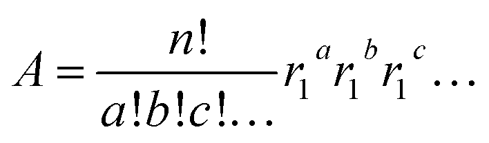
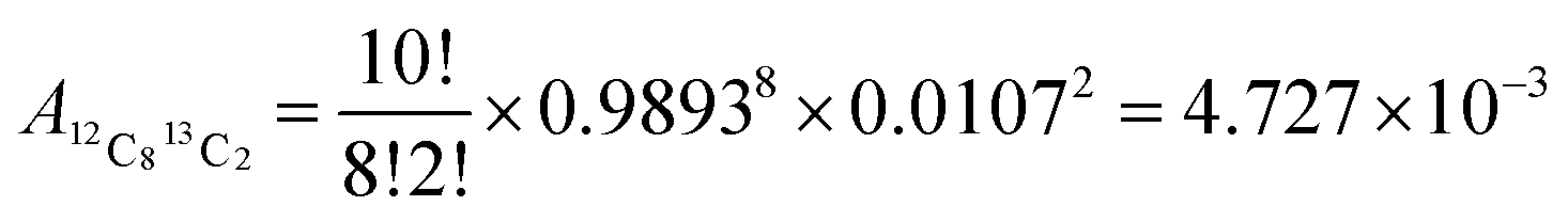
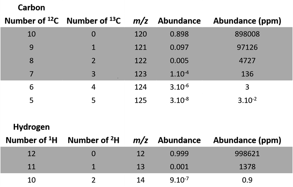
This method was developed with natSm–EDTA and further applied to the other Ln complexes. Briefly, we first calculated the theoretical isotopic pattern of natSm–EDTA by convolution. Based on this initial convolution data, we then defined the matrix of the isotopic contributions of the ligand atoms H, C, N and O. By combining this latter matrix with the measured intensities in the mass spectra of natSm–EDTA, we established a system of equations to determine the natSm isotopic composition. Among the available convolution methods,16 we used the readily implemented Yergey's polynomial method17 taking into account the stoichiometry of the complex and the relative isotopic abundances using both International Union of Pure and Applied Chemistry (IUPAC) data for H, C, N and O18 and TIMS data measured at the laboratory for natSm13 (Table 1 and Fig. 1b). By applying the Yergey's convolution method, we calculated the theoretical mass spectrum of negatively monocharged natSm–EDTA (Fig. 1c).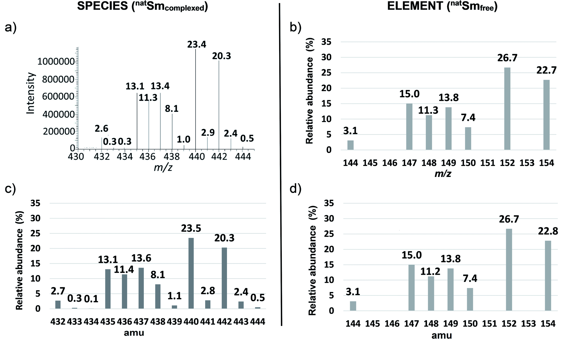 | ||
| Fig. 1 Isotopic patterns of natSm–EDTA and natSm (a) experimental mass spectrum of natSm–EDTA recorded by ESI-LIT-MS in full scan mode, (b) reference natSm isotopic pattern obtained by TIMS,13 (c) natSm–EDTA isotopic pattern calculated with the Yergey convolution method17 (d) natSm isotopic pattern obtained by deconvolution of the experimental ESI mass spectrum of natSm–EDTA. | ||
Except for Sm for which the stoichiometry is one, we calculated the atomic abundance of each isotopic permutation for each element using eqn (1):
 | (1) |
For example, one of the permutations of C10 is 12C813C2, leading to the atomic abundance of 4727 ppm (Fig. 2):
 | ||
| Fig. 2 Atomic abundance of carbon and hydrogen isotopic permutations for deprotonated EDTA (C10H12N2O8). | ||
We disregarded all permutations with abundances lower than 10 ppm for the next step of our study as they have a negligible impact on our calculations.
In a second step, the abundance of each permutation for natSm–EDTA was determined. It corresponds to the product of the abundance of the isotopic permutations of each element, calculated in the first step, by respecting the stoichiometry of the species. For example, the abundance of the 148Sm12C813C21H1214N216O718O1 permutation at m/z 440 was calculated according to eqn (2), resulting in 8.51 × 10⁻⁶:
| A148Sm12C813C21H1214N216O718O1 = A148Sm × A12C813C2 × A1H12 × A14N2 × A16O718O1 | (2) |
The third step consisted in summing the combined abundances of all the previous calculated permutations for each m/z ratio and Sm isotope. Table 3 gives the results in matrix form, with the m/z ratios of the natSm–EDTA in columns and the natSm isotopes in rows.
| Element | Species | |||||||||||||||||||
|---|---|---|---|---|---|---|---|---|---|---|---|---|---|---|---|---|---|---|---|---|
| 432 | 433 | 434 | 435 | 436 | 437 | 438 | 439 | 440 | 441 | 442 | 443 | 444 | 445 | 446 | 447 | 448 | 449 | 450 | 451 | |
| 144Sm | 2.7 × 10⁻² | 3 × 10⁻² | 1 × 10⁻³ | 5.9 × 10⁻⁵ | 6.2 × 10⁻⁶ | 4.7 × 10⁻⁷ | 2.1 × 10⁻⁸ | 6.4 × 10⁻¹⁰ | 4.6 × 10⁻¹² | 1.2 × 10⁻¹⁴ | 8.9 × 10⁻¹⁸ | |||||||||
| 147Sm | 0.3131 | 1.6 × 10⁻² | 0.003 | 2.9 × 10⁻⁴ | 3.0 × 10⁻⁵ | 2.3 × 10⁻⁶ | 1.0 × 10⁻⁷ | 3.1 × 10⁻⁹ | 2.2 × 10⁻¹¹ | 5.7 × 10⁻¹⁴ | 4.3 × 10⁻¹⁷ | |||||||||
| 148Sm | 9.8 × 10⁻² | 1.2 × 10⁻² | 2 × 10⁻³ | 2.1 × 10⁻⁴ | 2.2 × 10⁻⁵ | 1.7 × 10⁻⁶ | 7.6 × 10⁻⁸ | 2.3 × 10⁻⁹ | 1.7 × 10⁻¹¹ | 4.3 × 10⁻¹⁴ | 3.3 × 10⁻¹⁷ | |||||||||
| 149Sm | 0.121 | 1.4 × 10⁻² | 3 × 10⁻³ | 2.6 × 10⁻⁴ | 2.8 × 10⁻⁵ | 2.1 × 10⁻⁶ | 9.3 × 10⁻⁸ | 2.1 × 10⁻⁹ | 2.1 × 10⁻¹¹ | 5.2 × 10⁻¹⁴ | 4.0 × 10⁻¹⁷ | |||||||||
| 150Sm | 0.064 | 8 × 10⁻³ | 1 × 10⁻³ | 1.4 × 10⁻⁴ | 1.5 × 10⁻⁵ | 1.1 × 10⁻⁶ | 5.0 × 10⁻⁸ | 1.5 × 10⁻⁹ | 1.1 × 10⁻¹¹ | 2.8 × 10⁻¹⁴ | 2.1 × 10⁻¹⁷ | |||||||||
| 152Sm | 0.233 | 2.8 × 10⁻² | 5 × 10⁻² | 1 × 10⁻³ | 5.3 × 10⁻⁵ | 4.1 × 10⁻⁶ | 1.8 × 10⁻⁷ | 5.5 × 10−69 | 4.0 × 10⁻¹¹ | 1.0 × 10⁻¹³ | 7.7 × 10⁻¹⁷ | |||||||||
| 154Sm | 0.198 | 2.4 × 10⁻² | 5 × 10⁻³ | 4.3 × 10⁻⁴ | 4.5 × 10⁻⁵ | 3.4 × 10⁻⁶ | 1.5 × 10⁻⁷ | 4.7 × 10⁻⁹ | 3.4 × 10⁻¹¹ | 8.6 × 10⁻¹⁴ | ||||||||||
| Total | 0.03 | 0.00 | 0.00 | 0.13 | 0.11 | 0.14 | 0.08 | 0.01 | 0.23 | 0.03 | 0.20 | 0.02 | 0.00 | 0.00 | 0.00 | 0.00 | 0.00 | 0.00 | 0.00 | 0.00 |
| Abundance (%) | 2.7 | 0.3 | 0.1 | 13.1 | 11.4 | 13.6 | 8.1 | 1.1 | 23.5 | 2.8 | 20.3 | 2.4 | 0.5 | 0.0 | 0.0 | 0.0 | 0.0 | 0.0 | 0.0 | 0.0 |
By way of example, in the cell corresponding to m/z 440 and 148Sm, the abundances of all the permutations corresponding to this m/z with 148Sm (e.g. A148Sm12C813C21H1214N216O718O1 and A148Sm12C913C11H1214N115N116O718O1) were summed. The theoretical relative abundance for each m/z ratio of natSm–EDTA was then calculated by summing the values of each column. On the basis of these calculated abundances, the resulting theoretical natSm–EDTA isotopic pattern appears to be consistent with the experimental mass spectrum, as illustrated in Fig. 1a and c.
By considering the range of natural abundance variations provided by IUPAC for H, C, N and O,19 the maximum impact on calculated abundance ratios was ±1.4% for the natSm–EDTA ratio of 432/438, with the species at m/z = 432 containing the less abundant 144Sm isotope (3.1%). The difference was lower than 0.1% for the other isotope ratios. These variations were therefore considered to be negligible in this study. That being said, the theoretical bias, corresponding to the difference between experimental natSm–EDTA abundance ratios and calculated natSm–EDTA abundances ratios by convolution, was calculated for all abundance ratios of natSm–EDTA. This theoretical bias was better than 3% with repeatability of 3% for results obtained by ESI-QqQ-MS, and better than 1% with repeatability of 1% with the ESI-LIT-MS (data not shown). To determine the natSm isotopic composition by deconvolution of the experimental natSm–EDTA mass spectra obtained by ESIMS, the next step was to remove the isotopic contributions of H, C, N and O at each m/z ratio. For this, a system of n equations with n unknowns, was defined from the abundance matrix (Table 3) and further solved. In the case of natSm–EDTA, n is equal to 7, which represents the atomic abundances of the seven natSm isotopes. The H, C, N and O contributions for each m/z ratio were calculated by dividing each row of the matrix by the atomic abundance of corresponding natSm isotopes. A new matrix including only the H, C, N and O isotopic contributions from EDTA was then obtained (Table 4).
| H, C, N and O isotopic contributions | m/z ratio | ||||||
|---|---|---|---|---|---|---|---|
| 432 | 435 | 436 | 437 | 438 | 440 | 442 | |
| 144Sm | 0.873 | 1.907 × 10⁻³ | 1.989 × 10⁻⁴ | 1.518 × 10⁻⁵ | 6.713 × 10⁻⁷ | 1.493 × 10⁻¹⁰ | 2.887 × 10⁻¹⁶ |
| 147Sm | 0.873 | 0.105 | 2.0 × 10⁻² | 1.907 × 10⁻³ | 1.518 × 10⁻⁵ | 2.077 × 10⁻⁸ | |
| 148Sm | 0.873 | 0.105 | 2.0 × 10⁻² | 1.989 × 10⁻⁴ | 6.712 × 10⁻⁷ | ||
| 149Sm | 0.873 | 0.105 | 1.907 × 10⁻³ | 1.518 × 10⁻⁵ | |||
| 150Sm | 0.873 | 2.0 × 10⁻² | 1.989 × 10⁻⁴ | ||||
| 152Sm | 0.873 | 2.0 × 10⁻² | |||||
| 154Sm | 0.873 | ||||||
The natSm isotope ratios were then determined from the measured intensities (I) of the natSm–EDTA isotopic pattern and the contribution matrix of the H, C, N, O isotopes at each m/z ratio, by defining a system of 7 equations, with the 7 unknowns being the atomic abundances of natSm isotopes.
For example, for m/z 432 and m/z 435 (Table 4 and eqn (3)):
| 432I = 0.873 × 144A and 435I = 1.907 × 10−3 × 144A + 0.873 × 147A | (3) |
The natSm isotope ratios were then determined by combining the obtained atomic abundances. An example is given below for the 147Sm/144Sm ratio (eqn (4)):
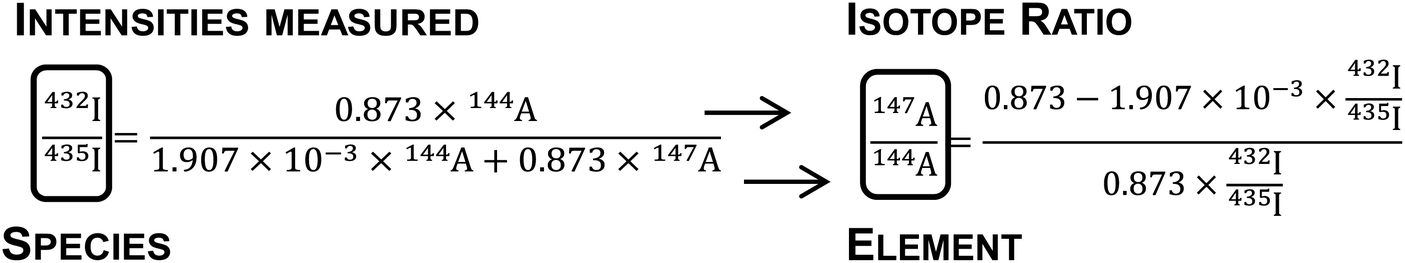 | (4) |
Determination of isotopic composition of lanthanides contained in chemical species by ESIMS
The experimental mass spectra of natSm–EDTA (Fig. 1a) were deconvoluted to obtain the isotopic pattern of natSm (Fig. 1d). The results are given in Table 5, together with the reference isotope ratios of natSm, the trueness, calculated as the difference between experimental natSm isotope ratios obtained after deconvolution and the reference natSm isotope ratios, as well as the repeatability of the measurements.| natSm isotope ratios | 144Sm/150Sm | 147Sm/150Sm | 148Sm/150Sm | 149Sm/150Sm | 152Sm/150Sm | 154Sm/150Sm | |
|---|---|---|---|---|---|---|---|
| TIMS reference value13 | 0.4194 | 2.0365 | 1.5257 | 1.8739 | 3.6173 | 3.0733 | |
| ESI-QqQ-MS | Average (n = 10) | 0.4062 | 1.9799 | 1.4976 | 1.8502 | 3.6264 | 3.0474 |
| Trueness (%) | −3.1 | −2.8 | −1.8 | −1.3 | 0.3 | −0.8 | |
| Repeatability (%) | 2.2 | 1.2 | 2.8 | 2.0 | 1.5 | 1.9 | |
| ESI-LIT-MS | Average (n = 10) | 0.4166 | 2.0376 | 1.5296 | 1.8718 | 3.6216 | 3.0860 |
| Trueness (%) | −0.7 | 0.1 | 0.3 | −0.1 | 0.1 | 0.4 | |
| Repeatability (%) | 1.0 | 0.9 | 0.7 | 0.9 | 0.7 | 0.7 | |
The bias before deconvolution, calculated as the difference between the experimental natSm–EDTA abundance ratios and the reference natSm isotope ratios, ranged between 8 and 24%. After deconvolution, the natSm isotope ratios were determined with a trueness better than 3.5% and a repeatability of about 3% for ESI-QqQ-MS, and a trueness better than 1.0% and a repeatability of about 1% for ESI-LIT-MS.
The same approach was applied to a double spike enriched in 147–149Sm of known isotopic composition and complexed with EDTA. The isotopic composition of 147–149Sm was then determined from the 147–149Sm–EDTA mass spectra recorded with ESI-QqQ-MS and ESI-LIT-MS.
This double spike was selected since 147–149Sm–EDTA leads to a more complex spectrum than natSm–EDTA for the less abundant Sm isotopes (Fig. 1a and 3a).
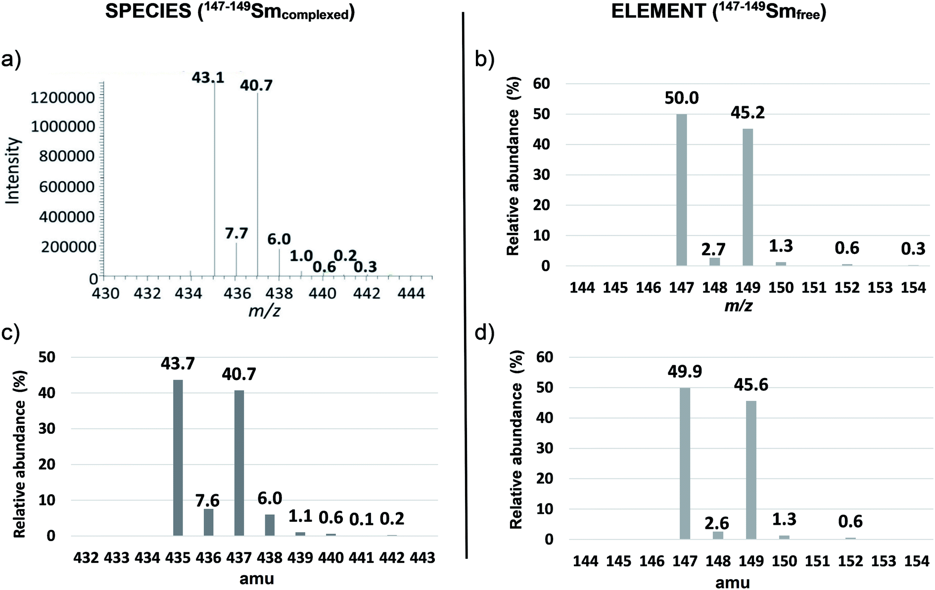 | ||
| Fig. 3 Isotopic patterns of 147–149Sm–EDTA and 147–149Sm (a) experimental mass spectrum of 147–149Sm–EDTA recorded by ESI-LIT-MS in full scan mode, (b) reference 147–149Sm isotopic pattern obtained by TIMS,14 (c) 147–149Sm–EDTA isotopic pattern calculated with the Yergey convolution method,17 (d) 147–149Sm isotopic pattern obtained by deconvolution of the experimental ESI mass spectrum of 147–149Sm–EDTA. | ||
In particular, the less abundant Sm isotope of natSm (144Sm) led to 2.7% abundance at m/z 432 in the natSm–EDTA convoluted spectrum (Fig. 1c). This mass was not impacted by the H, C, N and O isotopic contributions because it is associated with the lightest Sm isotope. The abundances in the natSm–EDTA spectrum ranging between 8.1 and 23.5% (Fig. 1c) are associated with Sm isotopes with abundances ranging between 7.4 and 26.7% (Fig. 1b). Conversely, there are two major ions with abundances of 43.7 and 40.7% at m/z 435 and m/z 437 in the 147–149Sm–EDTA convoluted spectrum (Fig. 3c). These peaks are related to 147Sm and 149Sm isotopes with abundances of 50.0 and 45.2% (Fig. 3b). The other Sm isotopes showed much lower abundances (less than 2.7%) and were all significantly impacted by the H, C, N and O isotopic contributions. In particular, the relative abundances of 148Sm and 150Sm were 2.7% and 1.3% (Fig. 3b), and 7.6% and 6% respectively for m/z 436 and m/z 438 in the 147–149Sm–EDTA isotopic pattern (Fig. 3c).
As the theoretical bias calculated with m/z 435 as reference was systematically positive with ESI-LIT-MS for the 148Sm–EDTA/147Sm–EDTA ratio and for all abundance ratios of 147–149Sm–EDTA with ESI-QqQ-MS (data not shown), we attributed these interferences to the residual nitrates coming from the sample preparation. To remove such interference, corrections detailed in the experimental part were applied. After correction, the theoretical bias and the repeatability at k = 2 were better than 2% and 4% with ESI-QqQ-MS (data not shown), for all abundance ratios for which Sm isotope abundances were greater than 1%. With ESI-LIT-MS, the theoretical bias and the repeatability were better than 2% for all abundance ratios, except for the 152Sm–EDTA/147Sm–EDTA ratio, for which the theoretical bias was about 9%, because of the too low intensity of the signal. The experimental ESI-LIT-MS mass spectra of 147–149Sm–EDTA (Fig. 3a) were deconvoluted to obtain the 147–149Sm isotopic composition (Fig. 3d). Table 6 gives the isotope ratios of 147–149Sm determined after deconvolution of mass spectra, the reference 147–149Sm isotope ratios, the trueness and the repeatability of the measurements.
| 147–149Sm isotope ratios | 148Sm/147Sm | 149Sm/147Sm | 150Sm/147Sm | 152Sm/147Sm | |
|---|---|---|---|---|---|
| TIMS reference value14 | 0.0534 | 0.9035 | 0.0253 | 0.0113 | |
| ESI-QqQ-MS | Average (n = 3 × 10) | 0.0531 | 0.9135 | 0.0258 | 0.0061 |
| Trueness (%) | −0.6 | 1.1 | 2.0 | −46.3 | |
| Repeatability (%) | 9.3 | 3.0 | 12.9 | 7.5 | |
| ESI-LIT-MS | Average (n = 3 × 10) | 0.0524 | 0.9136 | 0.0253 | 0.0125 |
| Trueness (%) | −2.0 | 1.1 | 0.3 | 10.4 | |
| Repeatability (%) | 1.8 | 0.2 | 2.5 | 2.1 | |
The bias before deconvolution for the major 149Sm–EDTA/147Sm–EDTA abundance ratio was around 4% with the two ESI instruments, whereas it was between 25% and 450% for the minor abundance ratios. After deconvolution, we achieved a trueness better than 2% with the two instruments, except for the 152Sm/147Sm ratio for which the 152Sm abundance was 0.6% (Fig. 3d). For this ratio, trueness was worse than 10%. With ESI-QqQ-MS, the repeatability was 3% for the major 149Sm/147Sm ratio, while it was about 10% for the other ratios. With ESI-LIT-MS, the repeatability was better than 2.5% for all isotope ratios. These results confirm the validity of all the isotopic measurements we performed with commercial ESIMS instruments as well as the readily implementable deconvolution method, for isotopes of relative abundances greater than 1% in samples. The 147–149Sm isotope ratios were determined by ESI-QqQ-MS and ESI-LIT-MS with a trueness better than 3% for Sm isotope ratios ranging between 0.025 and 0.9 with isotope abundances as low as 1.3%. This is true despite the strong impact of the H, C, N and O isotopic contributions from adjacent major peaks 20 to 40 times more intense.
We further carried out isotopic measurements starting with ESI mass spectra of chemical species containing another lanthanide (natNd–EDTA), another ligand (natSm–DTPA) and different lanthanide and ligand (natNd–DTPA). The isotope ratios of natNd and natSm were then determined by applying the deconvolution method to the associated lanthanide complexes and compared to reference ratios of the free lanthanides. The isotope ratios of natNd determined after deconvolution of natNd–DTPA mass spectra (Fig. S1†), the reference natNd isotope ratios, the trueness and the repeatability of the measurements are given in Table 7, while the results obtained for natNd–EDTA and natSm–DTPA are provided in Tables S1 and S2, as well as in Fig. S2 and S3.†
| natNd isotope ratios | 142Nd/144Nd | 143Nd/144Nd | 145Nd/144Nd | 146Nd/144Nd | 148Nd/144Nd | 150Nd/144Nd | |
|---|---|---|---|---|---|---|---|
| TIMS reference value13 | 1.1397 | 0.5110 | 0.3487 | 0.7233 | 0.2430 | 0.2382 | |
| ESI-QqQ-MS | Average (n = 10) | 1.1304 | 0.5090 | 0.3479 | 0.7205 | 0.2444 | 0.2391 |
| Trueness (%) | −0.8 | −0.4 | −0.2 | −0.4 | 0.6 | 0.4 | |
| Repeatability (%) | 2.1 | 2.1 | 2.1 | 1.4 | 2.1 | 2.4 | |
| ESI-LIT-MS | Average (n = 10) | 1.1225 | 0.5089 | 0.3451 | 0.7228 | 0.2432 | 0.2366 |
| Trueness (%) | −1.5 | −0.4 | −1.0 | −0.1 | 0.1 | −0.7 | |
| Repeatability (%) | 0.3 | 0.4 | 0.5 | 0.3 | 0.3 | 0.4 | |
For all abundance ratios of natNd–DTPA measured by ESI-QqQ-MS and ESI-LIT-MS, a bias between 0 and 30% was obtained before deconvolution in comparison with reference natNd isotope ratios obtained by TIMS.13 After deconvolution of the natNd–DTPA mass spectra, the natNd isotope ratios were determined with a trueness better than 1% and a repeatability of around 2% with ESI-QqQ-MS, and a trueness better than 1.5% and a repeatability of around 0.5% with ESI-LIT-MS (Table 7).
These results indicate that the performance of natNd isotope ratio measurements obtained from ESI mass spectra of natNd–DTPA are very good and similar to those measured for the natSm–EDTA species, by retaining the same experimental parameters.
By deconvolution of the mass spectra of natNd–EDTA and natSm–DTPA, the isotope ratios of the natLn were determined with a trueness better than 3.0% and a repeatability of around 2.5% with ESI-QqQ-MS, and a trueness better than 2.5% and a repeatability of around 0.5% with ESI-LIT-MS (Tables S1, S2, Fig. S2 and S3†). Overall, we were able to demonstrate that the substitution of Sm by Nd in the EDTA or DTPA chemical species has no impact either on the quality of the isotopic measurements with the two ESIMS instruments, or on the performance of the deconvolution method that we developed.
This work was carried out using model samples but can be performed with more complex samples, by coupling a separation step to ESIMS, to isolate the chemical species and the potential interferents before the analysis step.
Conclusion
The aim of the present work was to determine the isotopic composition of elements contained in chemical species, by electrospray mass spectrometry. In particular, the isotopic composition of natural and non-natural Sm and natural Nd contained in EDTA and DTPA complexes, were determined using two different mass spectrometers. To meet this aim, we developed a user-friendly deconvolution method to directly determine the Ln isotopic composition based on ESI mass spectra of the associated chemical species, by removing the isotopic contributions of the atoms from the ligand without performing fragmentations experiments by tandem mass spectrometry. By applying the deconvolution method to the mass spectra of Sm–EDTA species containing natural and enriched samarium, a trueness and a repeatability globally better than 3% were obtained for all isotope ratios of Sm with isotope abundances greater than 1%, using ESI-QqQ-MS and ESI-LIT-MS. The performance of the 147–149Sm–EDTA abundance ratio measurements and deconvolution method demonstrated the approach applicability for non-natural sample analysis; including low-abundance isotopes strongly impacted by H, C, N, and O isotopic contributions from the major neighbouring isotopes. The deconvolution method was also successfully applied to other Ln–polyaminocarboxylic species such as natNd–EDTA, natSm–DTPA and natNd–DTPA, leading to similar performance of trueness and repeatability. This approach can be extended to the isotopic characterization of elements contained in any chemical species by electrospray mass spectrometry, and appears therefore to be promising for the use this technique by its own for elemental speciation analysis. The implementation of this approach to LC-ESIMS coupling is of great interest for the comprehensive speciation study of elements in various fields. Such comprehensive speciation is of great concern in applications associated with the nuclear fuel cycle for the development of spent fuel treatment processes, in nuclear toxicology to study the effect of radioelements at the cellular and molecular level and design specific decorporation agents, in geosciences to determine the distribution processes of contaminants chelated to different organic ligands in environmental compartments and in life sciences to better understand the mechanisms underlying the toxicity of metals.Conflicts of interest
There is no conflict of interest to declare.Acknowledgements
The authors would like to acknowledge the CEA for its financial support.References
- D. M. Templeton, F. Ariese, R. Cornelis, L.-G. Danielsson, H. Muntau, H. P. Van Leeuwen and R. Lobinski, Pure Appl. Chem., 2000, 72, 1453–1470 CAS.
- D. M. Templeton and H. Fujishiro, Coord. Chem. Rev., 2017, 352, 424–431 CrossRef CAS.
- EGADSNF, Paris, France, OECD, NEA/NSC/WPNCS/DOC, 2011, 5.
- D. Schaumlöffel and A. Tholey, Anal. Bioanal. Chem., 2011, 400, 1645–1652 CrossRef PubMed.
- S. Miah, S. Fukiage, Z. A. Begum, T. Murakami, A. S. Mashio, I. M. M. Rahman and H. Hasegawa, J. Chromatogr. A, 2020, 1630, 461528 CrossRef CAS PubMed.
- L. Beuvier, C. Bresson, A. Nonell, L. Vio, N. Henry, V. Pichon and F. Chartier, RSC Adv., 2015, 5, 92858–92868 RSC.
- M. J. Keith-Roach, Anal. Chim. Acta, 2010, 678, 140–148 CrossRef CAS PubMed.
- R. Jirásko and M. Holčapek, Mass Spectrom. Rev., 2011, 30, 1013–1036 CrossRef PubMed.
- C. Shiea, Y. L. Huang, S. C. Cheng, Y. L. Chen and J. Shiea, Anal. Chim. Acta, 2017, 968, 50–57 CrossRef CAS PubMed.
- M. E. Ketterer and J. P. Guzowski, Anal. Chem., 1996, 68, 883–887 CrossRef CAS PubMed.
- M. C. B. Moraes, J. G. A. Brito Neto and C. L. do Lago, J. Anal. At. Spectrom., 2001, 16, 1259–1265 RSC.
- C. Liu, B. Hu, J. Shi, J. Li, X. Zhang and H. Chen, J. Anal. At. Spectrom., 2011, 26, 2045–2051 RSC.
- J. C. Dubois, G. Retali and J. Cesario, Int. J. Mass Spectrom. Ion Process., 1992, 120, 163–177 CrossRef CAS.
- M. Bourgeois, H. Isnard, A. Gourgiotis, G. Stadelmann, C. Gautier, S. Mialle, A. Nonell and F. Chartier, J. Anal. At. Spectrom., 2011, 26, 1660–1666 RSC.
- J. Kragten, Analyst, 1994, 119, 2161–2165 RSC.
- K. Scheubert, F. Hufsky and S. Böcker, J. Cheminform, 2013, 5, 1–24 CrossRef PubMed.
- J. A. Yergey, Int. J. Mass spectrom. Ion Physics, 1983, 52, 337–349 CrossRef CAS.
- M. Berglund and M. E. Wieser, Pure Appl. Chem., 2011, 83, 397–410 CAS.
- J. Meija, T. B. Coplen, M. Berglund, W. A. Brand, P. De Bièvre, M. Gröning, N. E. Holden, J. Irrgeher, R. D. Loss, T. Walczyk and T. Prohaska, Pure Appl. Chem., 2016, 88, 293–306 CAS.
Footnotes |
| † Electronic supplementary information (ESI) available. See DOI: 10.1039/d0ja00471e |
| ‡ Current address: Normandie Univ, UNIROUEN, Ecodiv, 76000 Rouen, France. |
| § Current address: Departament de Dinàmica de la Terra i de l'Oceà, Facultat de Ciències de la Terra, Universitat de Barcelona, 08028 Barcelona, Spain. |
| This journal is © The Royal Society of Chemistry 2021 |