
 Open Access Article
 This Open Access Article is licensed under a
 Creative Commons Attribution 3.0 Unported Licence
Transmission line revisited – the impedance of mixed ionic and electronic conductors†
Andreas E.
Bumberger
 ,
Andreas
Nenning
and
Juergen
Fleig
*
,
Andreas
Nenning
and
Juergen
Fleig
*
Institute of Chemical Technologies and Analytics, TU Wien, Vienna, Austria. E-mail: juergen.fleig@tuwien.ac.at
First published on 8th May 2024
Abstract
This contribution provides a comprehensive guide for evaluating the one-dimensional impedance response of dense mixed ionic and electronic conductors based on a physically derived transmission line model. While mass and charge transport through the bulk of a mixed conductor is always described by three fundamental parameters (chemical capacitance, ionic conductivity and electronic conductivity), it is the nature of the contact interfaces that largely determines the observed impedance response. Thus, to allow an intuitive adaptation of the transmission line model for any specific measurement situation, the physical meanings of terminal impedance elements at the ionic and electronic rail ends are explicitly discussed. By distinguishing between charge transfer terminals and electrochemical reaction terminals, the range of possible measurement configurations is categorized into symmetrical, SOFC-type and battery-type setups, all of which are explored on the basis of practical examples from the literature. Also, the transformation of an SOFC electrode into a battery electrode and the relevance of side reactions for the impedance of battery electrodes is discussed.
Introduction
Electrochemical impedance spectroscopy (EIS) has become an indispensable tool for studying the thermodynamic and kinetic properties of mixed ionic and electronic conductors (MIECs). In the field of solid-state ionics, the most prominent classes of MIECs include intercalation electrodes for batteries (e.g. Li1−δCoO2 (LCO)), high-temperature mixed-conducting electrodes for solid oxide cells (e.g. La0.6Sr0.4CoO3−δ (LSC)), and imperfect electrolytes (e.g. gadolinium-doped ceria (GDC) or Li0.29+δLa0.57TiO3 (LLTO) under reducing conditions). By applying a low-amplitude voltage or current perturbation onto an electrochemical system, impedance spectroscopy allows the separation of transport processes in the frequency domain according to their characteristic time constants. Generally, the more chemically and morphologically complex a system, the larger the variety of transport processes and time constants that potentially contribute to the overall impedance spectrum. As a result, intricate equivalent circuits with a large number of parameters are required to adequately describe the impedance response of, for example, a porous lithium-ion battery (LIB) or solid oxide fuel or electrolyser cell (SOFC/SOEC) electrode.1–4However, even if morphological complexities such as porosity or tortuosity can be excluded and a well-defined, single-crystalline MIEC sample is measured, the analysis of the recorded impedance spectra is often far from trivial, mainly for two reasons. First, although the bulk electrochemical properties of a mixed conductor are described by only three independent parameters (see below), these can vary over orders of magnitude, depending on the chemical potential of the relevant neutral species. For example, the electrochemical properties of LIB electrode materials are strongly dependent on the state-of-charge (SOC), i.e. the Li content.5–7 Analogously, the transport properties of SOFC and SOEC materials vary with the oxygen content.8 The second reason for the large variety of MIEC impedance spectra is found in the boundary conditions for ionic and electronic transport at the contact interfaces, which necessarily contribute to the measured impedance spectra. In the simplest case, the contacts are either fully blocking or reversible (non-blocking) for ions and/or electrons. Unfortunately, this qualitative black-and-white distinction is rarely realized in experiments, meaning that the magnitudes of the corresponding interfacial resistances and capacitances for both ionic and electronic charge carriers must be taken into account.
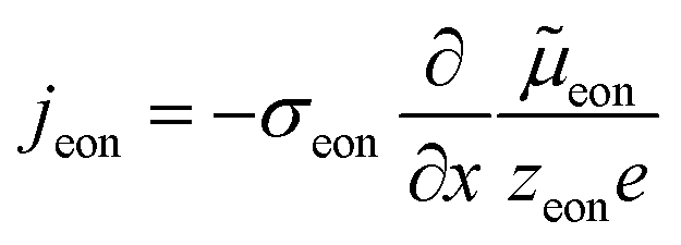
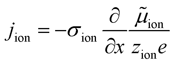
The extraction of physically meaningful solid-state electrochemical properties from an MIEC impedance spectrum requires an equivalent circuit that is based on the underlying differential equations describing the transport of mass and charge in the presence of electrical and chemical potential gradients. The one-dimensional particle flux density Ji of a charged species i is described by the Nernst–Planck equation,9,10 which reads
 | (1) |
As first proposed by Jamnik and Maier,13–15 and later in a more comprehensive form by Lai and Haile,9 these problems can be circumvented by mapping eqn (1) itself onto an equivalent circuit before applying any simplifying assumptions or boundary conditions. For a one-dimensional current flow across an MIEC slab of area A and thickness L, this results in a general transmission line circuit, featuring two parallel resistive rails for ion and electron conduction with small resistive increments rion and reon, which are coupled by incremental chemical capacitors cchem, as shown in Fig. 1a. The total ionic and electronic resistances are thus given by Rion = ∑rion, Reon = ∑reon, and the total chemical capacitance is Cchem = ∑cchem. At the rail ends, terminal impedance elements Zi account for the interfacial processes of ions and electrons taking place at the contact/MIEC boundaries. In many cases, R|C elements may be used to describe the terminal impedances Zi, cf.Fig. 1b and c. The dielectric bulk capacitance Cdiel of the MIEC is connected in parallel to the entire transmission line.
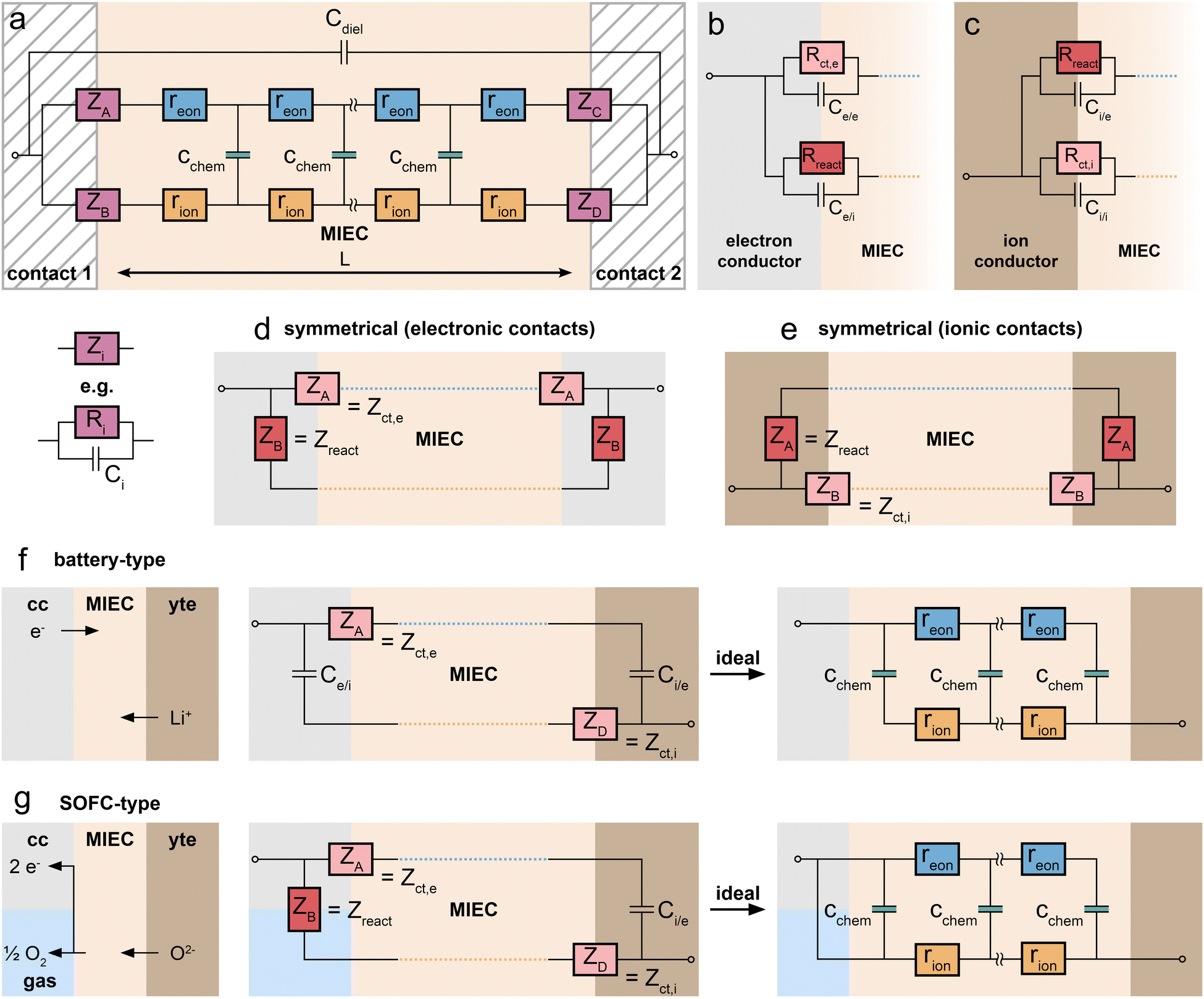 | ||
| Fig. 1 (a) General one-dimensional transmission line model for the transport of mass and charge across a MIEC slab of area A and thickness L. The circuit consists of two parallel resistive rails for electronic and ionic transport, coupled by chemical capacitors. Two different contacts define the terminal impedances for electrons (ZA, ZC) and ions (ZB, ZD). The bulk dielectric capacitance of the MIEC is connected in parallel to the transmission line. (b) Terminal impedance elements at the interface between electron conductor and MIEC. (c) Terminal impedance elements at the interface between ion conductor and MIEC. (d) Schematic representation of a symmetrical measurement setup with electronic contacts. (e) Schematic representation of a symmetrical measurement setup with ionic contacts. (f) Sketch and interfacial impedance elements of a battery-type setup, with the MIEC sandwiched between current collector (cc) and electrolyte (yte). (g) Sketch and interfacial impedance elements of an SOFC-type setup, with the MIEC sandwiched between current collector/oxygen atmosphere and electrolyte. The idealised circuits on the r.h.s. of (f) and (g) neglect interfacial capacitances and resistances. | ||
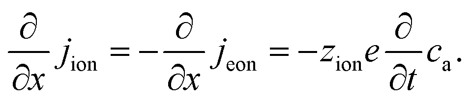
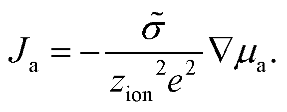
The equivalence of this transmission line and the underlying transport equations becomes more visible when expressing the electronic and ionic current densities (jeon, jion) by the gradients of electrochemical potentials of the respective species (∇![[small mu, Greek, tilde]](https://www.rsc.org/images/entities/i_char_e0e0.gif) eon,∇ion) with i = μi + zieΦ, μi being the chemical potential of species i. In the one-dimensional case we then have
eon,∇ion) with i = μi + zieΦ, μi being the chemical potential of species i. In the one-dimensional case we then have
 | (2) |
 | (3) |
 | (4) |
An analytical impedance expression of the transmission line circuit was originally only derived for symmetrical contacts,9i.e. for ZA = ZC, ZB = ZD. However, the impedance of the circuit can also be expressed analytically for the general case of four different Zi by adapting the derivation in ref. 9 for four distinct terminals.16 This is essential for inherently non-symmetrical MIEC devices such as battery electrodes. The full impedance expression of the transmission line in Fig. 1a can be found in ref. 16 and is also provided in a slightly modified nomenclature as ESI† to this paper in the form of a Matlab script. The reader is encouraged to use this script for simulations and explore how the impedance spectrum changes in response to a variation of interface and material parameters. Furthermore, the equivalent circuit has been implemented in the impedance analysing software ZView upon request (distributed element DX type 34).
In contrast to the underlying differential equations, the general transmission line can easily be adapted and simplified for specific experimental situations and also allows a physically meaningful integration of the solid-state transport impedance into larger equivalent circuits. Moreover, it provides a highly intuitive approach to understanding the impedance of MIECs and a common root for the impedance responses of different types of MIEC devices. However, this relies on a correct and physically meaningful interpretation and use of the terminal impedances, which is not always straightforward and requires further considerations.
In this contribution, we provide a practical guide for applying the transmission line model to a wide range of measuring geometries and devices commonly encountered in solid-state electrochemical research, including batteries, solid oxide cells and symmetrical two-electrode setups for the characterisation of MIECs and solid electrolytes. The physical meanings of the terminal impedances are discussed and rules are introduced in order to help deciding which of the terminating R and C elements are essential or negligible in certain cases. We provide specific application examples from current research and also discuss the limitations of approaches that rely on traditional Warburg elements by relating them back to the transmission line model. Furthermore, we emphasize the close relationship between different types of MIEC devices and show how minor experimental adjustments may transform the transmission line from one device type to another. Thus, our work is aimed at improving the intuitive understanding of MIEC impedance spectra and providing a practical approach for the derivation of tailored equivalent circuits for any specific experimental situation.
Interfacial impedances and specification of case studies
In principle, MIECs might be contacted by other MIECs, by ionic conductors (electrolytes) or by electron conductors (e.g. metals). Here, we restrict ourselves to the (very common) cases of MIECs being contacted either by a pure electron conductor or a pure ion conductor. Then, one charge carrier can move directly between contact and MIEC, whereas the other carrier can only enter or leave the MIEC if an electrochemical coupling reaction at the interface takes place. As a consequence, also the electrochemical processes causing the interfacial impedances of the two rails become different. In other words: ZA and ZB (or ZC and ZD) are fundamentally different. This is specified in the following.For the charge carrier that can also move in the contact material (electrons in a metal contact, ions in an electrolytic contact), the resistive part of the corresponding interfacial impedance is “simply” a charge transfer resistance between two phases. We thus denote this terminal impedance as “charge transfer impedance” Zct. Space charge regions but also chemical energy barriers between the two phases may play a crucial role here. For electrons, for example, the situation can be very similar to a Schottky contact on a semiconductor. In many cases this charge transfer impedance may be described by a charge transfer resistance Rct in parallel to an interfacial capacitance. The latter is charged by changing the interfacial charge carrier concentrations in both phases, for example by changing the corresponding space charge(s). These changes, however, only refer to the charge carrier which is mobile in both phases (e.g. electrons for an electronic contact) and are denoted as Ce/e and Ci/i for the electronic or ionic rail, respectively.
The charge carrier in the MIEC which cannot move in the contact material (e.g. ions in the electronic contact) has fundamentally different boundary conditions. The only way to still get a DC current of this charge carrier in the MIEC via the respective rail is by means of an electrochemical reaction, which couples the ions in the MIEC to the electrons in the contact or vice versa. For graphical differentiation, this element (Zreact) is drawn vertically. For oxygen ion conducting MIECs, a typical electrochemical coupling reaction is the oxygen exchange reaction 1/2O2 + 2e− ⇌ O2−, for example at a porous metal electrode. For a metal ion conducting MIEC, on the other hand, reduction of a metal ion and its deposition on the electrode may take place. The reaction Li+ + e− ⇌ Li0, for example, enables a Li+ current without any contact of the MIEC to a lithium-ion conductor.
This second type of interfacial terminal impedance may exist on both rails, for the ionic rail at the electronic contact and for the electronic rail at the ionic contact. We label it reaction or coupling impedance Zreact, and its resistive part is represented by the resistance Rreact, which reflects the kinetics of the corresponding electrochemical reaction. In parallel to this resistor, again a parallel capacitor Ci/e (or Ce/i) comes into play. This capacitor, however, resembles more the electrolytic double layer capacitance known from electrochemistry, with ions accumulating at one side of the interface and electrons on the other. In Fig. 1b and c, the two different types of interfaces are sketched, both with two different terminal elements. Interfaces without any electrochemical reaction lead to infinitely large coupling resistances Rreact. The corresponding charge carrier is then fully blocked and the terminating impedance is reduced to a capacitor. Interfaces with finite coupling resistances are (at least partly) transmissive for the corresponding charge carrier. However, it should be noted that the treatment of the four terminal impedances as R|C elements is an approximation of the exact, usually not analytically solvable set of boundary conditions.14
Having clarified the different types of terminating elements, we may now specify typical measurement situations. When analysing the material properties of an MIEC, we often rely on a (geometrically) symmetrical situation, i.e. the use of the same type of contact on both sides of the MIEC. This situation is sketched in Fig. 1d and e, where the reaction impedances Zreact are drawn in a vertical position to emphasise their role as coupling elements between the two resistive rails. Numerous examples of such symmetrical situations are discussed in this paper, first for a pure electrolyte and then for MIECs with either electrons or ions being blocked.
A very different situation is found for MIEC electrode materials used in lithium-ion batteries. It is far beyond the scope of this paper to consider the impedance of typical porous electrodes; for this the reader is referred to ref. 2 and 3. Here, we restrict our discussion to the very basic features of a dense MIEC used as a battery electrode in a one-dimensional manner. Contacting of such battery-type electrodes is asymmetrical per definition, as shown in Fig. 1f: on one side of the MIEC an electrolyte supplies ions and on the other side the current collector transfers electrons. Electrochemical (coupling) reactions at both contacts should be absent and the corresponding Zreact are thus essentially capacitive. Accordingly, the corresponding transmission line is antisymmetrical, at least in terms of circuit elements, even though the absolute values of the corresponding elements are generally different. If charge transfer resistances are negligible as well, the battery-type situation simplifies to the antisymmetrical circuit in Fig. 1f (r.h.s.), provided Cchem ≫ Ce/i and Ci/e, respectively.
This changes when moving to situations typical for MIEC electrode materials used in SOFCs/SOECs, such as (La,Sr)FeO3−δ (LSF), (La,Sr)CoO3−δ (LSC), (La,Sr)(Co,Fe)O3−δ (LSCF) or (La,Sr)MnO3−δ (LSM), etc. Again, we do not consider the case of porous electrodes with their complex interplay of mixed conduction, gas diffusion and electrochemical reaction. Rather, we restrict ourselves to quasi-one-dimensional electrodes (e.g. thin film electrodes), cf. sketch in Fig. 1g. On the electrolyte side of the MIEC, electrons should be completely blocked, i.e. electrochemical reactions should not occur at all. At the opposite (electronic current collector) side, however, ions should not be blocked in fuel cell application. Rather, electrochemical reactions have to take place, with Rreact being as low as possible.
More specifically, electrochemical reactions such as oxygen evolution or oxygen reduction according to 1/2O2 + 2e− ⇌ O2− have to occur at such electrode/contact interfaces. Accordingly, a truly asymmetrical situation results. Actually, this takes us to the limits of the one-dimensional model since the corresponding reactions do not take place at the current collector/MIEC interface but mostly at the free MIEC surface or at the three-phase boundary. In any case this violates the one-dimensionality of the current flow. However, with a proper positioning of current collectors we may still treat such MIECs in a one-dimensional manner when representing the electrochemical reaction at the corresponding MIEC/contact interface by the terminal impedance ZB = Zreact = Rreact|Ce/i.
These three prototypical situations are all further discussed and exemplified in the course of this paper. In particular, it is shown how the terminal elements can be treated, and often simplified, for specific situations and examples. First, however, we want to further specify the basic elements of the transmission line model, relate them to the chemical diffusion coefficient and discuss this also in the context of another transmission line model very common in the field – the Warburg impedance.
Solid-state diffusion and Warburg elements
Basic circuit elements and ambipolar transport
According to the transmission line model, three parameters describe the bulk properties of an MIEC – the chemical capacitance Cchem, the ionic conductivity σion, and the electronic conductivity σeon. The electronic and ionic conductivities can each be quantified by a mobility ui and a concentration of mobile charge carriers ci of charge number zi according to| σi = |zi|eciui. | (5) |
The volume-specific chemical capacitance is defined as13,14
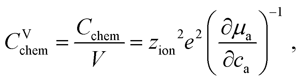 | (6) |
 | (7) |
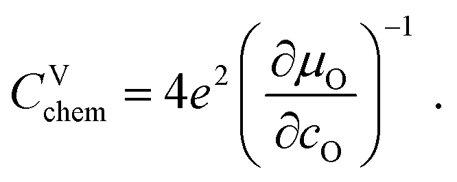
For LIB electrode materials, the stoichiometry change described by the chemical capacitance
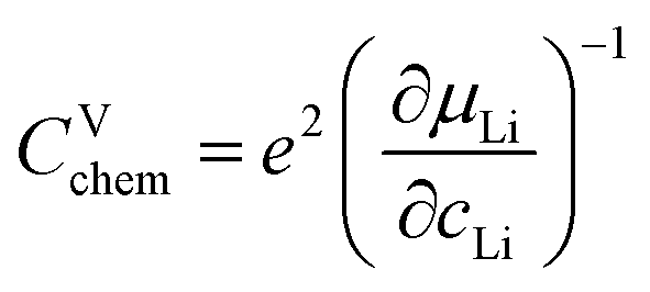 | (8) |
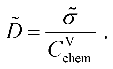
Obviously, on a phenomenological level, neutral atoms (either oxygen or lithium in the examples above) have to move in an MIEC to finally change its composition. This is realized by an electroneutral combined motion of ions and electrons, called ambipolar or chemical transport. This ambipolar transport can be quantified by two ambipolar properties – the ambipolar conductivity ![[small sigma, Greek, tilde]](https://www.rsc.org/images/entities/i_char_e10d.gif) and the ambipolar (or chemical) diffusion coefficient
and the ambipolar (or chemical) diffusion coefficient ![[D with combining tilde]](https://www.rsc.org/images/entities/i_char_0044_0303.gif) . The ambipolar conductivity
. The ambipolar conductivity
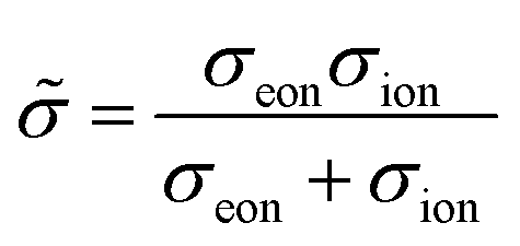 | (9) |
 | (10) |
The chemical diffusion coefficient describes the time dependence of stoichiometry changes according to Fick's law of diffusion
| Ja = −∇ca. | (11) |
 | (12) |
and CVchem may finally leave unperturbed.
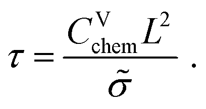
Assuming a one-dimensional geometry, i.e. transport across an MIEC slab of area A and thickness L, we thus find
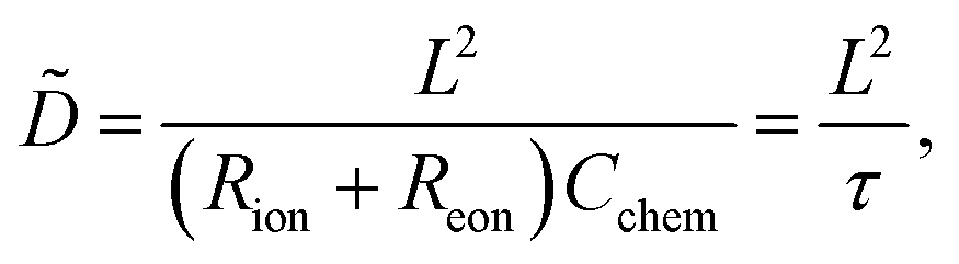 | (13) |
| τ = (Rion + Reon)Cchem | (14) |
 | (15) |
| τs = τ/4. | (16) |
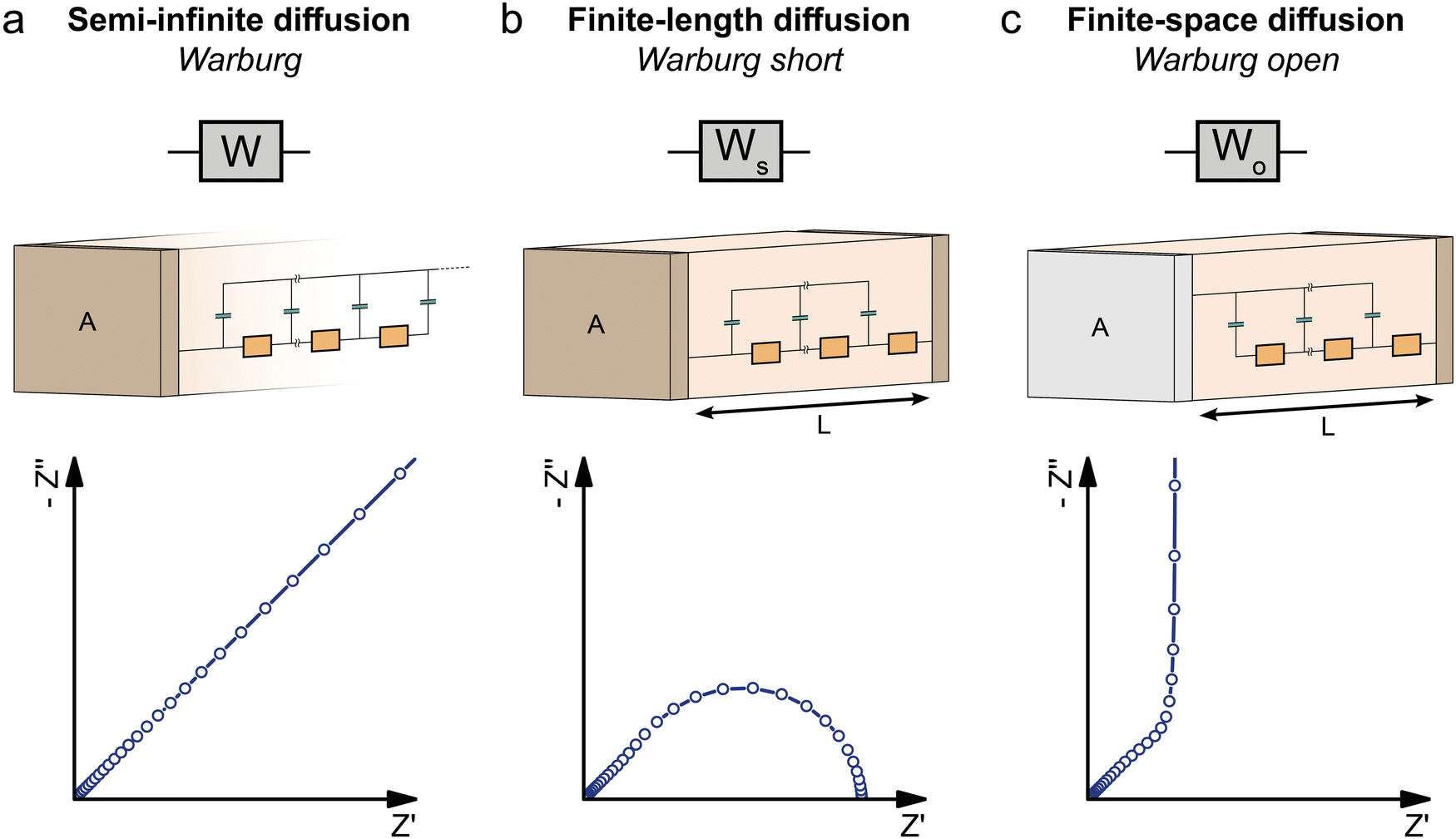 | ||
| Fig. 2 Different Warburg elements, their equivalent transmission lines, and their impedance responses, describing the impedance of concentration-driven diffusion for different boundary conditions. (a) Semi-infinite diffusion (Warburg). (b) Finite-length diffusion (Warburg short). (c) Finite-space diffusion (Warburg open). | ||
Warburg elements
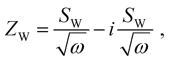
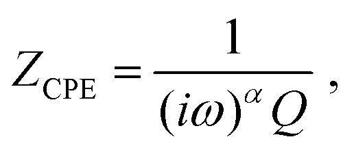
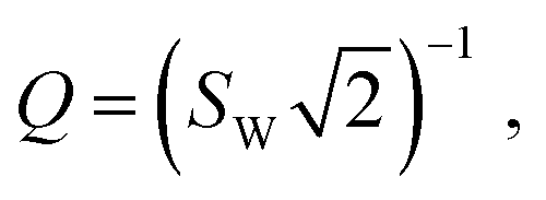
The impedance of diffusion processes has traditionally been accounted for in equivalent circuits by so-called Warburg elements. These circuit elements consider concentration gradients as the only driving force for mass transport. Thus, electrical potential gradients are neglected and eqn (1) is reduced to Fick's first law of diffusion, which can then be solved analytically for the appropriate boundary conditions and expressed as a current density to derive an impedance expression.In the transmission line picture, the Warburg impedance is a special case where one charge carrier has negligible resistance, and all terminal impedances are either short or open circuits. By variation of the boundary conditions, three different cases result: semi-infinite diffusion, finite-length diffusion and finite-space diffusion. In the following, we briefly summarize the three different Warburg elements, their impedance expressions and their equivalent circuit forms.
Semi-infinite diffusion considers the diffusion of particles from an infinite distance towards a transmissive boundary. In practice, this means that the sample thickness is large enough, or the diffusional resistance is high enough, for spatial limitations not to become relevant within the low-end frequency range of the impedance measurement. The corresponding impedance expression can be derived as19
 | (17) |
 | (18) |
 | (19) |
 | (20) |
 | (21) |
 | (22) |
 | (23) |
When the sample is thin enough, or the diffusional resistance low enough, for spatial limitations to become relevant within the low-end frequency range of the impedance measurement, boundary conditions need to be considered for both sides of the sample. For the case that both boundaries are fully transmissive for the diffusing species, the limiting impedance for ω → 0 is real and corresponds to the total diffusional resistance R (e.g. R = Rion for concentration-driven ion diffusion through an MIEC with Reon ≈ 0). Thus, in the low-frequency limit, the impedance is independent of frequency. This situation is often referred to as finite-length diffusion (see Fig. 2b), and for diffusing ions its frequency-dependent impedance response is given by
 | (24) |
If only one boundary is transmissive for the diffusing particles and the other blocks mass transport, the limiting impedance for ω → 0 is purely capacitive with a real offset corresponding to Rion/3 (for Reon ≈ 0) meaning that only the capacitive part of the impedance is frequency dependent in the low-frequency limit.11 This situation is referred to as finite-space diffusion and for diffusing ions results in the impedance expression
 | (25) |
In the following, the general transmission line from Fig. 1a will be applied to a variety of different measurement setups involving MIECs and electrolytes. Wherever appropriate, references will be made to the Warburg elements presented above, highlighting their relation to the general MIEC transmission line, but also their limitations.
Symmetrical measurements
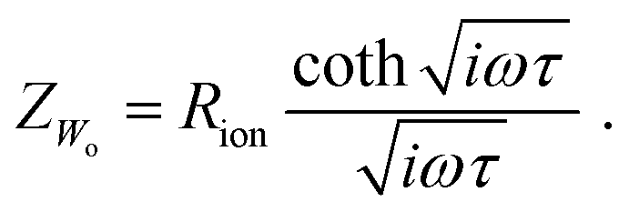
Symmetrical impedance measurements on electrolytes and MIECs constitute the simplest class of measurements that can be rationalized from a transmission line perspective. For their interpretation, it is usually enough to consider the analytical expression given by Lai and Haile for a symmetrical transmission line with ZA = ZC and ZB = ZD,9 which is less cumbersome than the general expression for four different terminals.Ion-blocking contacts on electrolytes
First, let us consider symmetrical impedance measurements on ideal electrolytes with negligible electronic conductivity in the context of the general MIEC transmission line model. Such measurements often use purely electron conducting contacts and their main purpose is the characterisation of an electrolyte's ionic conductivity. Typical experimental setups include in-plane20–23 and cross-plane24,25 measurements on thin films, bulk single crystals and polycrystals.26–28 In either case, we consider a slab of electrolyte sandwiched between two identical electronically conducting contacts.Due to the negligible electronic conductivity of the electrolyte (Reon → ∞), the electronic rail of the transmission line model in Fig. 1a can be discarded including its terminal elements, and thus also Cchem is negligible. The remaining circuit is shown in Fig. 3a. This approach to the equivalent circuit also emphasizes that the only way ions can lead to a DC current is via coupling reaction resistances Rreact. If the contacts present a completely blocking boundary to ions from the electrolyte, this coupling resistance on the ionic rail becomes infinitely large (Rreact → ∞), leaving only the interfacial capacitances Ce/i at the contact interfaces. Experimentally, this is (approximately) realized, for example, when contacting a sample of a Li+ solid electrolyte such as lithium phosphorous oxynitride (LiPON) with two Ti electrodes, as shown schematically in Fig. 3b. Assuming two identical Ti contacts, the transmission line is thus reduced to a simple equivalent circuit consisting only of Cdiel in parallel to a serial connection of Rion and the total interfacial capacitance Cint = Ce/i/2 as shown in Fig. 3b.
 | ||
| Fig. 3 (a) Adapted transmission line for an ideal ionic conductor (electrolyte) between two identical contacts. (b) Schematic sketch, equivalent circuit and simulated impedance response of LiPON between two ideal (ion-blocking, RB,RD → ∞) Ti contacts. The impedance spectrum consists of a high-frequency semicircle (Rion|Cdiel) and a capacitive line at low frequencies. (c) Measured impedance of a symmetrical Ti|LiPON|Ti thin film sample. Image reprinted from ref. 29 with permission from Elsevier. (d) Schematic sketch, equivalent circuit and simulated impedance response of LLZO between two Li contacts. The impedance spectrum consists of two semicircles corresponding to Rion|Cdiel and Rint|Cint. (e) Measured impedance of an LLZO pellet contacted by two Li electrodes. Image reprinted (adapted) from ref. 30 with permission from RSC Publishing. (f) Measured impedance of a YSZ pellet contacted by two LSC thin film electrodes covered with Pt paste. Diagram reproduced using data from ref. 26. A sample sketch was added for clarity. | ||
Since dielectric capacitances are typically much lower than interfacial capacitances (Cdiel ≪ Cint), the resulting impedance response ideally consists of a high-frequency bulk semicircle (Rion|Cdiel) which transitions into purely capacitive behaviour (Rion + Cint) at lower frequencies. In consequence, the quality of separation between these two regimes depends on the relative magnitudes of Cdiel and Cint. The former often also contains stray capacitances from the experimental setup (for example, from the substrate in in-plane measurements on a thin film) and Cdiel can therefore deviate from the bulk dielectric capacitance of the electrolyte.20,23 Further deviations from the ideal impedance spectrum in Fig. 3b can arise from imperfect ion blockage by the contacts (i.e. finite Rreact).26 Since the high-frequency semicircle corresponds to the bulk impedance response of the electrolyte (or MIEC), it is commonly referred to as the bulk semicircle.
For example, Fig. 3c shows the temperature-dependent cross-plane impedance response of a LiPON thin film sandwiched between two ion-blocking Ti electrodes, taken from ref. 29. The impedance spectra are very close to the ideal behaviour expected from Fig. 3b, with a bulk semicircle followed by a nearly vertical line due to the blocking interfacial capacitance of the contacts. The minor slope of the capacitive line can be accounted for by replacing the corresponding capacitance in the equivalent circuit by a constant-phase element, which allows for a more accurate fit of the bulk semicircle, especially in cases where the two features are not as well separated as in Fig. 3c.
If the contacts are partially transmissive for ions, the finite terminal resistances Rreact on the ionic rail in Fig. 3a have to be taken into account together with the corresponding interfacial capacitance Ce/i. Accordingly, we get the total interfacial capacitance Cint = ½Ce/i and the total interfacial resistance Rint = 2Rreact. The resulting equivalent circuit exhibits a similar impedance response as two serial R|C elements as long as the corresponding time constants are well separated, as shown in Fig. 3d. Experimentally, this situation can be realized by sandwiching an electrolyte between two reservoir electrodes that enable the required electrochemical reaction which couples the ionic to the electronic rail. In the context of LIB solid electrolytes, Li metal or a LiAl alloy are commonly used as the reservoir electrode, enabling the reaction Li+ + e− ⇌ Li. (Please note that in the alloying case, Rreact may not be sufficient for describing the relevant processes since diffusion in the alloy also comes into play.)
For example, Fig. 3e shows the impedance response of an Al-doped Li7La3Zr2O12 (LLZO) polycrystalline pellet with two symmetrical Li contacts, taken from ref. 30. As indicated in the figure, the high- and low-frequency semicircles correspond to the LLZO bulk (∼Rion|Cdiel) and Li electrodes (∼Rint|Cint) respectively, where Rint corresponds to the charge-transfer resistances at the two Li/LLZO interfaces.
For O2− electrolytes, on the other hand, contacts enabling oxygen exchange (e.g. via 1/2O2 + 2e− ⇌ O2−) are required, e.g. porous Pt electrodes. Fig. 3f shows the example of an yttria-stabilized zirconia (YSZ) single crystal symmetrically contacted by Pt paste electrodes, taken from ref. 26. This leads to a bulk semicircle (∼Rion|Cdiel) at high frequencies and an electrode feature at low frequencies. In this case, however, the high- as well as the low-frequency feature is far from an ideal semicircle and thus constant phase elements are required for an appropriate fit. Please note that on oxide ion conductors often mixed conducting electrodes are used, which may further complicate the terminal impedances. For measurements on polycrystals, an additional impedance feature due to grain boundaries is often found, which is not considered by the transmission line in Fig. 3a. For a more detailed discussion of the impedance contribution of grain boundaries, the interested reader is referred to the specialized literature.20,31–33
Ion-blocking contacts on MIECs
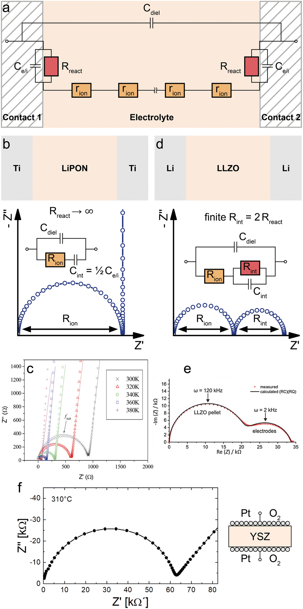
If the electronic and ionic conductivities are both significant, the material classifies as an MIEC. A determination of the corresponding material parameters in the transmission line (σeon, σion, Cchem) is then often based on measurements using the symmetrical cells shown in Fig. 1d and e, with further specified terminal elements ZA and ZB. Let us first consider the case of electron conducting contacts. Ideally, the charge transfer resistance of the electrons is negligible, Rct,e → 0, while the electrodes are completely blocking for ions, Rreact → ∞, as sketched in Fig. 4a. Then, the terminal impedance ZA is negligible and ZB reduces to the interfacial capacitance Ce/i (Fig. 4b). Even for a finite Rct,e the corresponding parallel capacitance Ce/e is often neglected, since it leads to an overparameterisation of the impedance fit. | ||
| Fig. 4 (a) Schematic sketch of a mixed ionic and electronic conductor between two ideal (ion-blocking) metal contacts. (b) Adapted transmission line corresponding to the sample sketch in subfigure (b). (c)–(h) Simulated impedance responses of the above transmission line circuit for different relative magnitudes of Ce/iversus Cchem and σionversus σeon. (i) Temperature-dependent impedance spectrum of an NMC523 pellet between two ion-blocking Ag contacts. Original image published in ref. 34 under a CC BY-NC-ND license. (j) In-plane impedance of an STF thin film under reducing conditions measured between two interdigitated Pt contacts. Original image published in ref. 35 under a CC BY license. (k) Measured impedance response of an NVPF pellet between two Ti contacts. Image reprinted (adapted) from ref. 36 with permission from ACS Publications. (l) Impedance spectrum of an Fe:STO thin film between a Nb:STO substrate and a Pt top contact. Original image published in ref. 37 under a CC BY license. (m) Impedance response of an STO single crystal between two Pt contacts. Diagram reproduced using data from ref. 38. (n) Temperature-dependent impedance response of an LSGM single crystal between two Pt contacts. Original image published in ref. 39 under a CC BY license. For subfigures (i), (l), (m), and (n), sample sketches were added for clarity. | ||
The shape of the resulting impedance spectrum strongly depends on the relative magnitudes of σeonversus σion and Cchemversus Ce/i, as well as on the portion of the impedance response that is accessible within commonly measured frequency ranges. Please note that the following discussion in terms of σion/σeon and Ce/i/Cchem is equivalent to the viewpoint of carrier mobilities and concentrations adopted in ref. 13 (Fig. 7), since these are related viaeqn (5) and (6).
Electronic charge carrier mobilities are typically much higher than for ionic carriers, and thus many MIECs are predominantly electronic conductors, such that σion ≪ σeon applies. Examples of such materials include many LIB and SOFC cathode materials such as LCO, LiMn2O4 (LMO), LSF or LSC.5,7,8,40,41 In some cases, both conductivities are of a similar magnitude (σeon ≈ σion), for example, in heavily Tb-doped YSZ,42 or Sr(Ti,Fe)O3−δ (STF).43 Examples of MIECs with predominant ionic conductivity are mostly encountered in the context of non-ideal electrolytes, such as partially reduced LLTO or GDC,44,45 and often limited to certain stoichiometric regions. An example of an insertion electrode material with predominant ionic conductivity is stoichiometric Na3V2(PO4)2F3 (NVPF),36,46 a cathode material for Na-ion batteries.
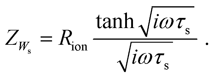
For MIECs with similar ionic and electronic conductivities such as highly Fe-doped STF at low pO2,35,43 the impedance response of the transmission line in Fig. 4b consists of two separate features that allow a simultaneous extraction of σion and σeon, as shown in Fig. 4e and f. The high-frequency semicircle corresponds to the bulk response of the mixed conductor, with the dielectric capacitance coupled to the effective bulk resistance Rbulk, which is related to the total conductivity σtot = σion + σeon according to
 | (26) |
. Thus, for ion-blocking contacts, a comparatively large low-frequency feature signifies σion > σeon and vice versa. The shape of the low-frequency feature may vary continuously between an ideal semicircle and a half-teardrop shaped Warburg feature, depending on the relative magnitudes of Ce/i and Cchem. For a relatively high chemical capacitance Ce/i ≪ Cchem, the low-frequency feature is identical to a finite-length Warburg element (Warburg short, cf.Fig. 2b) with a resistance RWs = Reon − Rbulk. This equivalence can also be shown mathematically by applying Ce/i = 0 (and Rct,e = 0) to the analytical impedance expression corresponding to the transmission line in Fig. 4b (see ref. 9, eqn (73)). Thus, the equivalent circuit can be further simplified into a serial connection of Rbulk and Ws parallel to Cdiel.
Such a circuit was applied, for example, in ref. 35, where the in-plane impedance of STF thin films on MgO was studied under reducing conditions using interdigitated Pt microelectrodes, as shown in Fig. 4j. Only the onset of the bulk semicircle can be seen at the highest frequencies, which transitions into the half-teardrop shape corresponding to Ws. Both features are of similar size, indicating very similar electronic and ionic conductivities of the material. Furthermore, the two features are well separated, allowing a further simplification of the circuit by neglecting the dielectric capacitance (Cdiel = 0) and treating the bulk semicircle as a high-frequency offset Rbulk. This way, σeon, σion, and Cchem could be extracted from the impedance data without having to implement a fit to the full transmission line.
For significantly different σion and σeon, the impedance spectrum is dominated either by the bulk semicircle (σion ≪ σeon) or the low-frequency feature (σion ≫ σeon). If both features are sufficiently resolved within the measured frequency range, the spectrum can be fitted using the full transmission line in Fig. 4b, or even the simplified circuit in Fig. 4e for Cint ≪ Cchem, to obtain all three bulk properties (σeon, σion, and Cchem).
For example, in ref. 37, the cross-plane impedance of 2% Fe-doped SrTiO3 (Fe:STO) thin films on Nb-doped SrTiO3 (Nb:STO) single crystals was studied using Pt microelectrodes (see Fig. 4l). The resulting impedance spectrum consists of a depressed low-frequency semicircle (apex frequency 358 Hz) and a significantly smaller high-frequency arc. By comparing the corresponding capacitances with the dielectric capacitance expected for the Fe:STO thin film, the high-frequency arc could be identified as the bulk semicircle originating from Rbulk coupled to Cdiel. Since the low-frequency feature does not exhibit a well-defined Ws behaviour, but is closer in shape to a semicircle, a fit of the full transmission line (Rct,e = 0) had to be applied, implying Ce/i > Cchem. In fact, the fit shown in Fig. 4l yields a value of Ce/i that is approximately one order of magnitude larger than Cchem, as can be deduced from the corresponding fit parameters given in the ESI of ref. 37. Please note that in this example, the interfacial capacitances were fitted as constant phase elements, and the values of Ce/i can only be estimated by converting the non-physical fit parameters Q and n into a corresponding capacitance (see, for example, ref. 31eqn (15)). As expected from the dominance of the low-frequency impedance feature, the Fe:STO thin film sample is a predominant ionic conductor, with σion being about two orders of magnitude higher than σeon. Thus, according to eqn (26), the effective bulk resistance Rbulk, which corresponds to the high-frequency arc, is virtually identical to Rion. At high frequencies, the predominant ionic conductor therefore behaves like an electrolyte (cf.Fig. 3b), with Reon → ∞, as shown in the inset of Fig. 4h. On the other hand, the resistance associated with the low-frequency feature can then be approximated by Reon − Rbulk ≈ Reon − Rion ≈ Reon. If either of the two impedance features is not sufficiently resolved to perform a reliable transmission-line fit, these approximations may be used to obtain either σion or σeon.
A very illustrative example is also given by Rupp et al. in ref. 39, where the temperature-dependent impedance of La0.95Sr0.05Ga0.95Mg0.05O3−δ (LSGM) single crystals is measured in synthetic air using symmetrical Pt contacts, as shown in Fig. 4n. The impedance response generally consists of a dominant Ws feature at low frequencies, indicating predominant ionic conductivity (σion ≫ σeon) together with a comparatively large chemical capacitance (Ce/i ≪ Cchem), and a much smaller bulk semicircle at high frequencies. The former and latter are only visible at high and low temperatures, respectively. Upon closer inspection, the 45° onset of the Ws feature contains an additional semicircle, which the authors attribute to a non-negligible electronic charge transfer resistance, terminating the electronic rail at the Pt|LSGM interface. In the transmission line in Fig. 4b, this corresponds to leaving two finite terminal resistances RA = RC = Rct,e at the electronic rail ends (cf.Fig. 1b, without corresponding capacitances Ce,e to avoid overparameterisation). Apart from the small Rct,e, the measured impedance response closely matches the simulated spectrum shown in Fig. 4g. At high temperatures (see ref. 39 for details), all time constants decrease, such that the low-frequency feature is fully contained in the measured frequency range (1 MHz to 5 mHz), but the bulk semicircle is beyond the high-frequency limit. Thus, the effective bulk resistance Rbulk is treated as a high-frequency offset and Cdiel is neglected. Since the electronic charge transfer semicircle is negligible at high temperatures, the spectra are fitted to a simple Rbulk + Ws circuit. At low temperatures (Fig. 4n), on the other hand, the bulk semicircle is fully visible, while only part of the 45° region of the Warburg feature is contained in the measured spectrum. Also, the charge transfer semicircle at mid frequencies is significant at low temperatures. As a consequence, these impedance spectra were fitted using the full transmission line from Fig. 4b, including RA = RC = Rct,e. However, since the low-frequency Warburg feature is not fully contained in the data, the corresponding fitting errors for Reon and Cchem exceed 100%.
The presence of such a non-negligible interfacial resistance Rct,e is even more evident in ref. 38, where the impedance of an STO single crystal between to Pt contacts is analysed. An exemplary spectrum, measured at a temperature of 600 °C and an oxygen partial pressure of 7 × 10⁻⁷ bar, is shown in Fig. 4m. Under these conditions, STO is a mixed conductor with σion similar to σeon, which is evident as the resistances associated with the high-frequency bulk and low-frequency Ws features are roughly within the same order of magnitude. In the mid-frequency range, an additional semicircle is clearly visible, which the authors attribute to a space charge resistance (Rs.c. = Rct,e) at the Pt/STO interfaces. Just like in the previous example of LSGM, the entire impedance spectrum with three arcs could therefore be fitted using a single transmission line (Fig. 4b), yielding an excellent quality of fit and physically meaningful material parameters.
An alternative approach to fitting a spectrum with a curtailed low-frequency Warburg feature, such as the one in Fig. 4n, is given in ref. 36. There, the mixed conductivity of the Na intercalation material NVPF is investigated by means of impedance spectroscopy using symmetrical Ti electrodes on a polycrystalline NVPF pellet, as shown in Fig. 4k. The resulting impedance response resembles that of the inset in Fig. 4g (Ce/i ≪ Cchem), with a high-frequency bulk semicircle (Rbulk|Cdiel) and a low-frequency 45° onset. Just like in the previous example of Pt|LSGM|Pt at low temperatures (Fig. 4m right), the full bulk semicircle is visible in the high-frequency region, while only the 45° portion of the low-frequency feature is contained in the measured data. Thus, it is not possible to perform a fit that yields reliable values for both σion and σeon. However, the dominant Warburg response at low frequencies indicates σion ≫ σeon, meaning that the bulk resistance associated with the high-frequency semicircle can be approximated as Rbulk ≈ Rion according to eqn (26). Thus, the ionic conductivity was obtained by fitting the spectrum with a simple Rion|Cdiel + W circuit, as shown in Fig. 4g. In this case, the fit parameters related to the semi-infinite Warburg element W are not further evaluated.
Finally, we consider the case of a predominant electronic conductor with σion ≪ σeon. The transmission line in Fig. 4b (Rct,e = 0) can then be simplified further by assuming Rion → ∞, resulting in a simple Reon|Cdiel circuit with a corresponding semicircle in the Nyquist plot (Fig. 4c and d). For example, in ref. 34 the impedance of a sintered pellet of LiNi0.5Mn0.2Co0.3O2 (NMC523) was measured for symmetrical silver contacts (Ag|NMC523|Ag) below 100 °C. The corresponding impedance spectra at two different temperatures are shown in Fig. 4i and exhibit the expected shape of a non-ideal semicircle, which is fitted using a Reon|Qdiel circuit to obtain the electronic conductivity. Again, the calculated impedance spectra in Fig. 4c and d principally consist of a high-frequency bulk semicircle, which is dominant for σion ≪ σeon, and a much smaller low-frequency feature, with a shape depending on the relative magnitudes of Ce/i and Cchem. However, due to the comparatively small resistance associated with this feature, it is often not visible in real impedance spectra, as in Fig. 4i.
Electron-blocking contacts on MIECs
Symmetrical impedance measurements with two electron-blocking contacts are experimentally much more challenging and therefore less common. Usually, such setups consist of a central MIEC sample to be characterized, sandwiched between a double layer of an ion conductor (inner layer = electron-blocking layer) and a reversible reservoir electrode (outer layer), as shown in Fig. 5a. The reservoir electrode acts as an elemental source and sink and is therefore required to be a low-impedance electrode such as Li metal or a reversible mixed conducting O2 electrode in the case of Li+ materials and SOFC materials, respectively. In other words, the reservoir electrode couples the ionic current across the electron-blocking layer and MIEC to the electronic current in the external circuit via an electrochemical reaction. Not surprisingly, this coupling reaction as well as mass and charge transport across the reservoir/electrolyte/MIEC interfaces is usually associated with non-negligible resistances, which contribute to the complexity of the measured impedance spectra. An additional resistance may arise from the finite ionic bulk conductivity of the electrolyte. Although all these contributions could be explicitly considered in the equivalent circuit, overlaps of the corresponding impedance features often limit their interpretability. Nonetheless, measurements on electron-blocking cells are an important complementary tool that can yield valuable, albeit often incomplete, information about the ambipolar conductivity of MIECs. In particular, the otherwise elusive ionic conductivity of predominant electronic conductors, such as most LIB cathode materials, can become accessible by this method.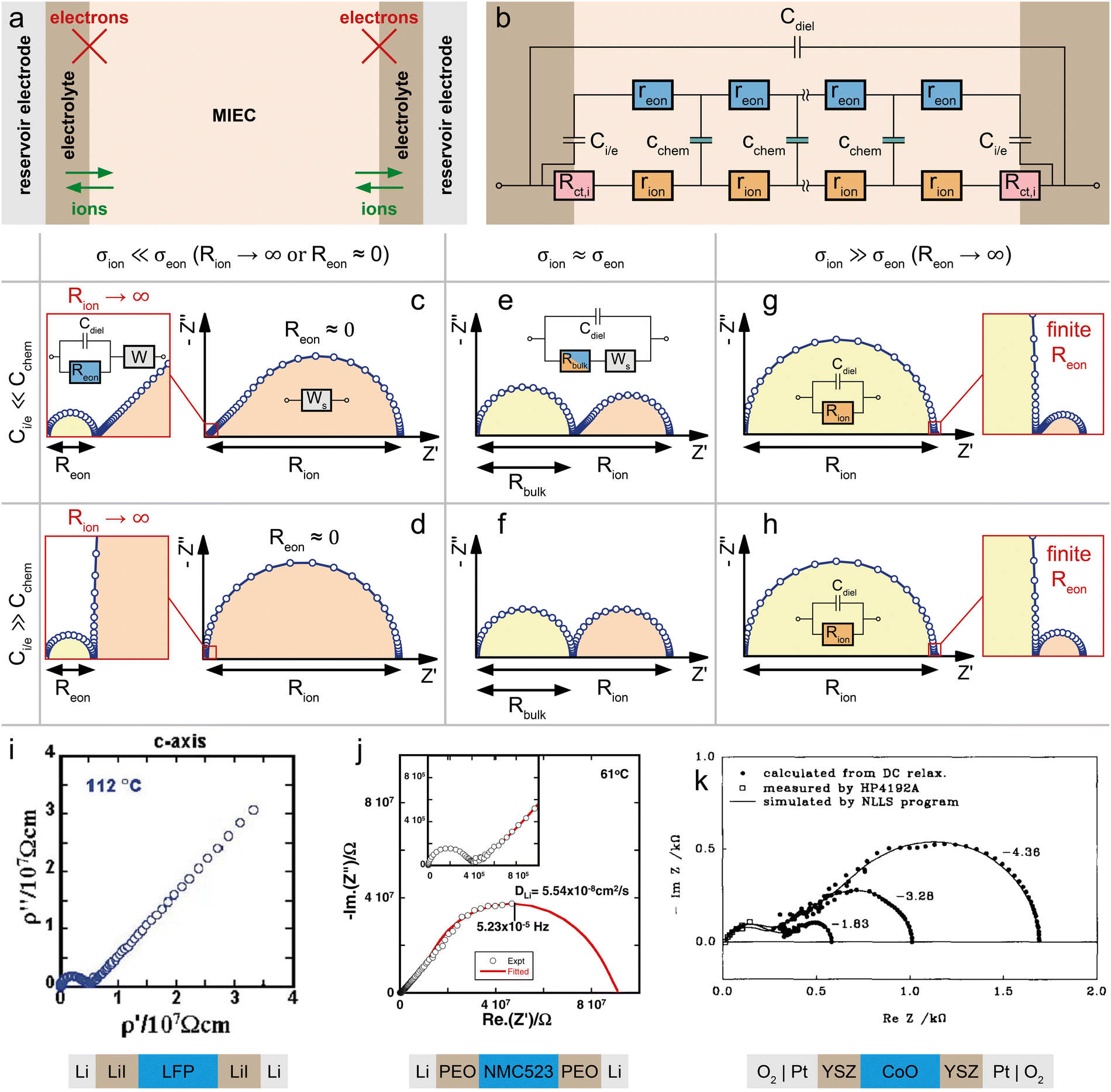 | ||
| Fig. 5 (a) Schematic sketch of a mixed ionic and electronic conductor between two ideal (electron-blocking) ion-conducting contacts. Reservoir electrodes are required to provide a contact to the external circuit. (b) Adapted transmission line corresponding to the sample sketch in subfigure (b), neglecting the outer reservoir electrodes. (c)–(h) Simulated impedance responses of the above transmission line circuit for different relative magnitudes of Ce/iversus Cchem and σionversus σeon. (i) Impedance response of a Li|LiI|LFP|LiI|Li cell, with a c-axis oriented LFP single crystal. Image reprinted from ref. 47 with permission from IOP Publishing. (j) Impedance response of a Li|PEO|NMC523|PEO|Li cell, with a sintered NMC523 pellet. Original image published in ref. 34 under a CC BY-NC-ND license. (k) Impedance response of a O2|Pt|YSZ|CoO|YSZ|Pt|O2 cell. In the low-frequency range, the data was obtained from DC relaxation measurements. Image reprinted from ref. 48 with permission from Elsevier. For subfigures (i)–(k), sample sketches were added for clarity. | ||
To understand the impedance response of the isolated electrolyte/MIEC/electrolyte cell, we start from the circuit of the symmetrical cells with ionic contacts in Fig. 1e. For complete electron blocking (Rreact → ∞) and a negligible ionic charge transfer resistance (Rct,i → 0), we end up with only one terminal element remaining, namely the coupling capacitance Ci/e. The resulting circuit is shown in Fig. 5b and is electrically equivalent to that for ion-blocking contacts in Fig. 4b.
As a result, also the calculated impedance response is inverted with respect to Rion and Reon, which becomes obvious when comparing the simulated spectra in Fig. 4 and 5. Just like for ion-blocking contacts, the impedance spectrum for a mixed conductor (σion ≈ σeon) consists of a high-frequency bulk semicircle and a low-frequency feature that takes the shape of either a Ws element (Ci/e ≪ Cchem) or a semicircle (Ci/e ≫ Cchem), as shown in Fig. 5e and f. While the bulk semicircle is still related to the effective bulk resistance Rbulk, the limiting DC resistance for ω → 0 is now given by Rion, such that the low-frequency feature is associated with a resistance Rion − Rbulk. In contrast to ion-blocking contacts, it is now the low-frequency feature that dominates the spectrum for predominant electronic conductors (σion ≪ σeon), since it indicates how much the blocked charge carriers (in this case electrons) contribute to the total conductivity. Its resistance can be approximated as Rion, while the much smaller bulk resistance is virtually identical to Reon (see Fig. 5c and d). For a predominant ionic conductor with σion ≫ σeon, on the other hand, the spectrum consists of a large bulk semicircle (∼Rion|Cdiel) and a much smaller low-frequency feature (see Fig. 5g and h).
For example, in ref. 47, the anisotropic electronic and ionic conductivity of LiFePO4 (LFP) single crystals is investigated by electron-blocking impedance measurements in a symmetrical Li/LiI/LFP/LiI/Li arrangement. A typical spectrum measured along the crystallographic c-axis at 112 °C is shown in Fig. 5i, consisting of a high-frequency semicircle and an extended 45° Warburg response at low frequencies, suggesting Ci,e ≪ Cchem. Although the low-frequency region is not fully contained in the spectrum, its associated resistance is apparently much larger than the semicircle, indicating σion ≪ σeon. The bulk resistance can therefore be approximated as Rbulk = Reon, with Rion → ∞, as shown in the inset of Fig. 5c, and the electronic conductivity can be extracted from the high-frequency semicircle. In that sense, the present example is fully analogous to the impedance spectrum of NVPF in Fig. 4k (ref. 36) measured with ion-blocking contacts. Importantly, however, the authors of ref. 47 note that the semicircle in Fig. 5i also contains ionic contact (“charge transfer”) impedances and minor contributions from the bulk conductivity of the electrolyte (LiI). Thus, the extracted values of σeon differ slightly from those obtained from measurements with ion-blocking metal contacts, highlighting the experimental difficulties associated with electron-blocking configurations.
A similar example is given in ref. 34, where the impedance of a sintered LiNi1/3Mn1/3Co1/3O2 (NMC111) pellet is measured in a symmetrical setup using doped polyethylene oxide (PEO) as the electrolyte (electron-blocking layer) and Li metal as the outer reservoir electrode. The resulting impedance spectrum at 61 °C is shown in Fig. 5j, again exhibiting a small high-frequency semicircle and a low-frequency Warburg response. In this case however, enough of the low-frequency region is contained in the spectrum to fit it as a Ws element with an associated resistance RWs = Rion − Rbulk, which the authors approximate as RWs ≈ Rion due to σion ≪ σeon (and thus Rbulk ≪ Rion) to extract the Li diffusivity and ionic conductivity. The high-frequency semicircle is assumed to contain contributions from the bulk conductivity of PEO in addition to Rbulk. Thus, since the electronic conductivity is more accurately determined by impedance measurements on ion-blocking cells (see Fig. 4i), the authors do not further consider this semicircle.
In principle, symmetrical impedance measurements with electron-blocking contacts can also be realized for oxygen ion conductors. For example, in ref. 48, a CoO bulk sample was sandwiched between two YSZ single crystals, which were covered with Pt paste on the outside. The latter couples the ionic current through the cell and the electronic current through the external circuit via the electrochemical oxygen exchange reaction with the surrounding atmosphere. Thus, Pt|O2 provides the reservoir electrode in analogy to Li metal in the previous examples. Although the low-frequency region of the resulting impedance spectra (Fig. 5k) was reconstructed from DC relaxation experiments, it nicely shows the impedance response of a predominant electronic conductor between two electron-blocking contacts, similar to Fig. 5c. Please note, however, that the semicircle observed at medium to high frequencies is attributed to the oxygen exchange impedance of the Pt|O2 electrode rather than the effective bulk resistance. The ionic conductivity of the mixed conductor is thus obtained by fitting the low frequency feature to a Ws element, in series to a high-frequency offset resistance (YSZ bulk resistance) and three R|Q elements to account for all interfaces, assuming Reon ≈ 0. Although meaningful values of σion could be obtained, the various interfacial contributions to the overall impedance highlight the complexity of such measurements and their interpretation.
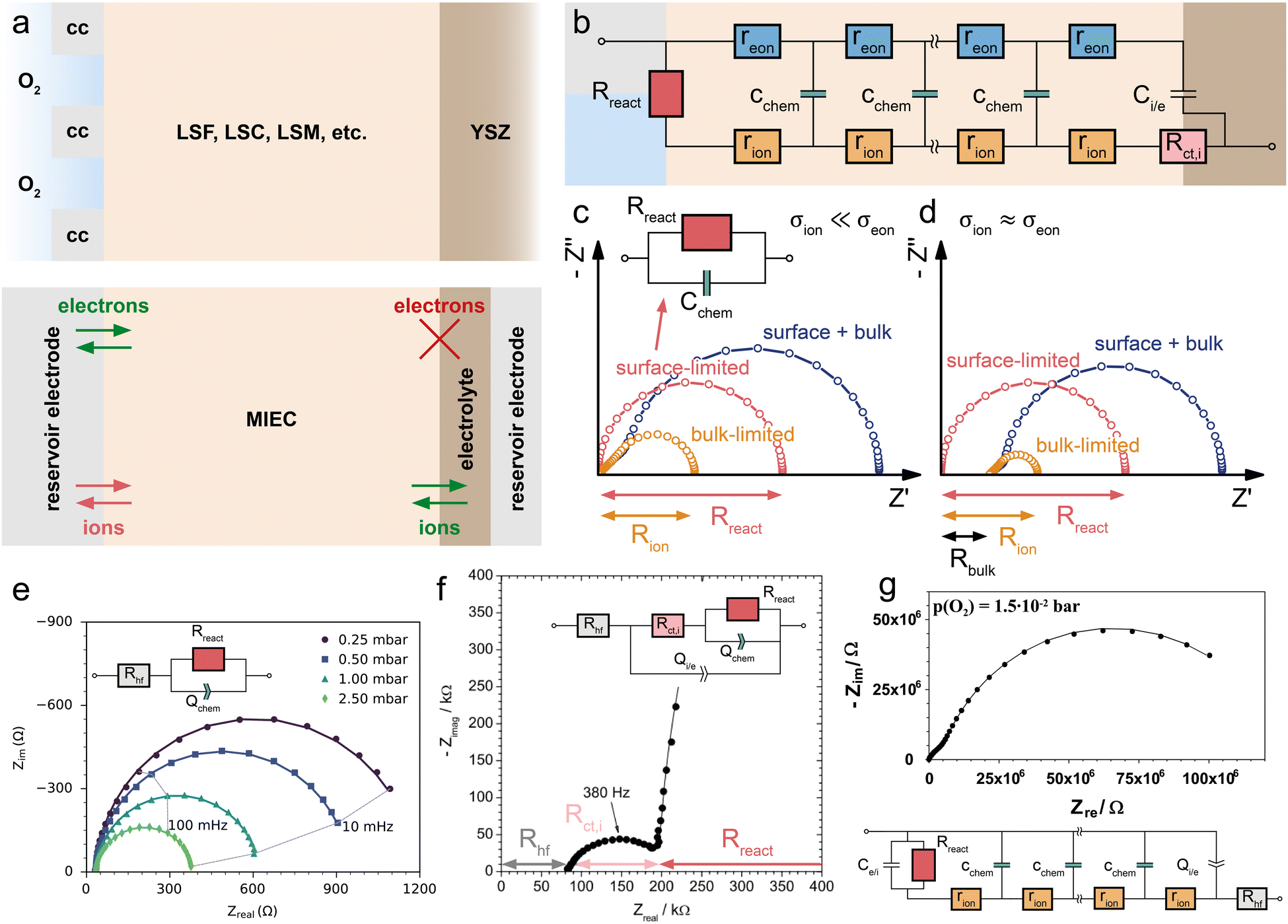
Measurements with SOFC-type contacting of MIECs
Mixed conducting electrodes in solid oxide fuel or electrolysis cells are always used with asymmetrical contacting, i.e. a current collecting electron conductor on one side and an electrolyte on the other side. The resulting circuit model with terminating elements was already discussed above and is shown in Fig. 1g. It is highly illustrative to simulate the impedance response of this transmission line (Fig. 1g) in order to better understand the impact of various terminal resistances and capacitances. However, such a detailed discussion of various possible combinations of contact selectivities and their effect on the general shape of the impedance spectrum is beyond the scope of this paper; it can be found in ref. 13 (Fig. 7b).Often, further simplifications are adequate and also required in order to avoid overparameterisation. In a typical simplification, we neglect both charge transfer resistances Rct,i and Rct,e and thus also the terminating impedances ZA and ZD. Moreover, Ce/i of the coupling impedance ZB = Zreact is often much smaller than Cchem and thus also neglected. Finally, we do not take the dielectric capacitance into account (or consider it only in parallel to any additional electrolyte resistance). This leads to the circuit shown in Fig. 6b, which can serve as the starting point for many considerations on quasi-one-dimensional (e.g. thin film) SOFC/SOEC electrodes.
 | ||
| Fig. 6 (a) Sketch (top) and schematic representation (bottom) of a dense SOFC electrode consisting of an MIEC on a YSZ electrolyte, with a current collector (cc) contacting the MIEC on the O2-exposed side. (b) Adapted transmission line for the SOFC electrode in subfigure (a). (c) Calculated impedance response of the SOFC electrode with a predominant electronic conductor (LSF, σion ≪ σeon) for different limiting cases. (d) Calculated impedance response of the SOFC electrode with a mixed conductor (STF at low pO2, σion ≈ σeon) for different limiting cases. (e) pO2-dependent half-cell impedance spectra of an LSF thin film grown on top of a Pt-grid current collector on a YSZ single crystal. Original image published in ref. 8 under a CC BY license. (f) Impedance response of an LSCF thin film microelectrode on a YSZ single crystal. Image reprinted (adapted) from ref. 49 with permission from Elsevier. (g) Impedance response of an LSM thin film microelectrode on a YSZ single crystal. Image reprinted (adapted) from ref. 50 with permission from John Wiley and Sons. For subfigures (e)–(g), the equivalent circuits used for impedance fits were added to the image. | ||
 | ||
| Fig. 7 (a) Schematic sketch of a dense SOFC electrode consisting of a predominant electronic conductor (LSF, σion ≪ σeon) on a YSZ electrolyte contacted by a current collector on the O2-exposed side. A capping layer blocks the surface exchange reaction between the O2 atmosphere and the LSF surface. (b) Evolution of the calculated impedance response (circuit Fig. 6b with Reon = 0) for an increasing surface exchange resistance Rreact due to the capping layer, showing the gradual transition from a Ws to a Wo type behavior. | ||
The coupling resistance in the ionic rail Rreact is of very high relevance for MIEC electrodes in SOFC/SOEC applications, since it describes the essential oxygen exchange kinetics of such electrodes. However, this resistance is also the reason that simplifications of the corresponding circuit by employing Warburg elements often fail. Accordingly, such measurements reveal the full potential of the transmission line model, which allows an intuitive description in the form of an equivalent circuit, while still being physically exact in terms of the Nernst–Planck equation eqn (1). In the following, several typical situations are discussed for important SOFC-materials, some of them allowing further simplifications, others requiring additional terminating elements, such as the ionic charge transfer resistance Rct,i = ZD in the ionic rail. At the end of this section, it is shown that a reaction resistance approaching very high values reflects the transition of a SOFC-type electrode to a battery-type electrode.
Solid oxide fuel and electrolysis cells
Fig. 6a sketches the situation under consideration – a dense SOFC cathode or SOEC anode, with the MIEC being in contact with the oxygen atmosphere and a current collector (O2|cc) on one side, and the O2− conducting electrolyte (e.g. YSZ) on the other side. The MIEC/electrolyte interface presents a fully blocking boundary for electrons, represented by Ci/e and may include an ionic charge transfer resistance Rct,i in the ionic rail. It is obvious from Fig. 6b that the impedance of the simplified equivalent circuit is limited by either surface exchange (Rreact) or bulk transport (Rion, Reon) (or ionic charge transfer Rct,i, if relevant).In the case of a predominant electronic conductor such as LSF, LSM or LSC, the resistances on the electronic rail can be neglected (Reon = 0), and the electrode's impedance response often falls into one of three categories, as shown in Fig. 6d. If the surface exchange resistance dominates and bulk transport resistances can be neglected (Rion = 0), a simple Rreact|Cchem semicircle results, which is observed, for example, for many SOFC thin film electrodes at high operating temperatures.40,41,49,51,52Fig. 6e exemplarily shows a set of pO2-dependent impedance measurements on an LSF thin film electrode, taken from ref. 8, which consist of a high-frequency offset due to the YSZ electrolyte resistance followed by a mid- to low-frequency Rreact|Qchem semicircle.
In many studies on such or similar thin film electrodes, however, an additional mid-frequency arc was observed, and in ref. 53 this was shown to be due to the ion transfer resistance at the MIEC/electrolyte interface Rct,i. Still neglecting all transport resistances (Rion = Reon = 0) leads to the equivalent circuit in Fig. 6f, which excellently fits the measured impedance spectra of many MIEC thin film electrodes on YSZ (with constant phase elements replacing the capacitors).
Next, we discuss the interplay of Rion and Rreact in the representative circuit Fig. 6b. In the case that the bulk transport resistance Rion is much higher than the surface exchange resistance (bulk-limited electrode), Rreact can be neglected and replaced by a short circuit. In the limit of negligible Reon and Ci/e, the resulting impedance response corresponds to a finite-length Warburg element (Fig. 2b). The crucial difference between the traditional Ws element and a bulk-limited SOFC electrode becomes visible once Rreact can no longer be neglected. While the traditional Ws element would imply a simple serial Ws + Rreact connection with a corresponding real-axis offset in the Nyquist plot, the physically more accurate transmission line in Fig. 6b predicts a merging of the surface resistance into the bulk transport feature, as shown in Fig. 6c (surface + bulk) by the emerging semicircle. In reality, the surface exchange resistance Rreact is rarely negligible compared to bulk transport resistances, at least not for Cchem ≫ Ce/i. Literature examples of dense SOFC or SOEC electrodes exhibiting only a simple Warburg impedance response are therefore hard to find.
An experimental example of a mixed surface-bulk-limited SOFC electrode can be found in ref. 50, where the partial pressure dependence and rate limiting steps of the oxygen reduction kinetics on LSM thin films is examined. The impedance response (Fig. 6g) consists of a low-frequency semicircle with a mid-frequency shoulder, which is ascribed to an ionic transport limitation across the LSM thin film at high oxygen partial pressures (i.e. low oxygen vacancy concentrations). The measured spectra were fitted using the transmission line shown in Fig. 6g, which is equivalent to the circuit in Fig. 6b for Rct,i = Reon = 0 with an additional high-frequency offset resistance Rhf and an interfacial capacitance Ce/i in parallel to the surface exchange resistance. The resulting fit allowed a separate analysis of the bulk transport and oxygen exchange kinetics in LSM.
For balanced mixed conductors with similar σion and σeon, such as STF at low pO2,43 the consideration of electronic bulk resistances requires the full transmission line (Fig. 6b). As shown in the simulated spectra of Fig. 6d, the impedance response is shifted by a real axis offset corresponding to Rbulk (eqn (26)) if the electronic bulk transport resistance cannot be neglected. Only in the surface-limited case, the impedance response is equivalent to that of a predominant electronic conductor, as it transforms into a simple Rreact|Cchem semicircle. Please note that the above discussion only considers the impedance response of the isolated MIEC sample and its interfaces. In reality, impedance spectra from two-electrode measurements usually contain additional contributions from, for example, the electrolyte and the counter electrode.41 However, these contributions can simply be considered in series to the MIEC impedance. Especially the electrolyte resistance is often well separated in the Nyquist plot, due to different time constants of the corresponding transport processes. Thus, their inclusion in the equivalent circuit is straightforward.
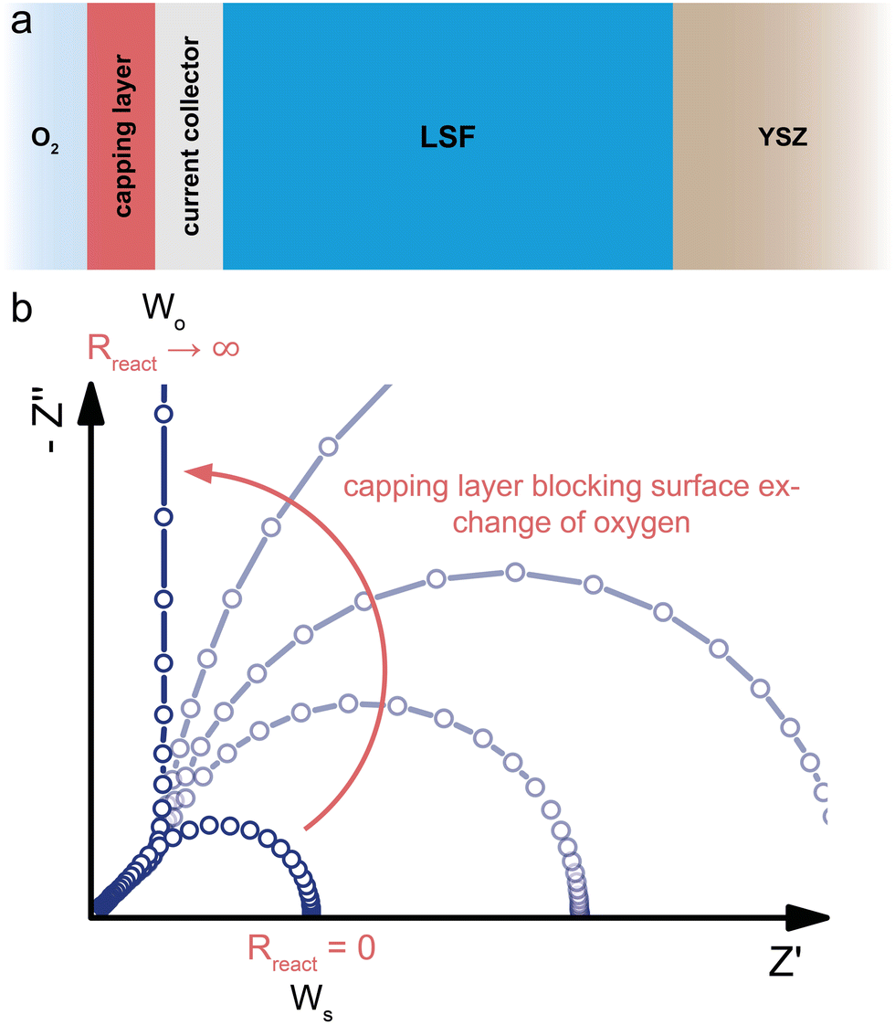
From SOFC to battery electrodes
A highly interesting transition occurs when the oxygen exchange reaction at an SOFC electrode surface is more and more blocked, as shown in Fig. 7. Starting from a bulk-limited electrode (Rreact = 0) of a predominant electronic conductor (Reon = 0), such as LSF, the impedance spectrum initially corresponds to that of a finite-length Warburg element (Ws) characterized by Rion and Cchem (Fig. 7b, cf. also Fig. 6c). When the oxygen surface exchange with the surrounding atmosphere is more and more blocked, Rreact increases. This can be achieved, for example, by covering the current collector and MIEC with a dense capping layer of negligible ionic conductivity. As a consequence, the impedance response first transitions away from the simple Ws element into a mixed regime, where both Rreact and Rion are relevant. For further increasing oxygen exchange resistances, the high frequency 45° part of the spectrum remains nearly unchanged, but the low frequency end transforms into a more and more separate semicircle dominated by the growing Rreact. If the capping layer is perfectly blocking (Rreact → ∞), the semicircle becomes infinitely large, such that it effectively transforms into a capacitor with a capacitance Cchem. For the transmission line in Fig. 6b, this implies that the connection between the left contact and the ionic rail of the MIEC can be considered as fully disrupted. Thus, the resulting circuit is equivalent to the transmission line representation of a finite-space Warburg element (Wo, Fig. 2c). However, for small Cchem, a coupling capacitor Ce/i might come into play at the current collector/MIEC interface.In terms of equivalent circuits, blocking the surface exchange reaction of an SOFC electrode corresponds to a transition from (quasi) finite-length (Ws) to finite-space (Wo) diffusion, with the intermediate region lying beyond the applicability of classical two-terminal Warburg elements. This emphasizes once more the consistency of the general transmission line model with the specific solutions to Fick's first law of diffusion for the respective boundary conditions, and shows that the separate consideration of ionic and electronic transport across the contact interfaces is required to accurately describe realistic measurement setups of SOFC electrodes with a finite, nonzero Rreact. In terms of device functionality, this transition constitutes the transformation of an SOFC electrode into an oxygen-ion battery electrode, which can store charge based on the principle of coulometric titration.17,54
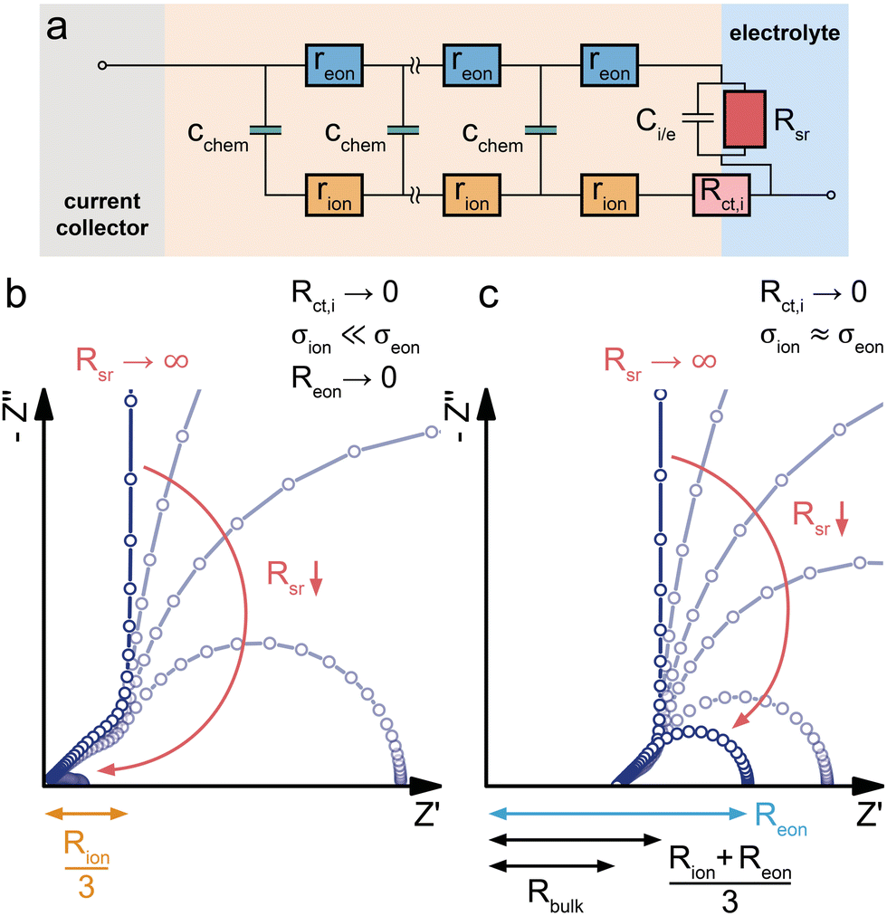
Measurements with battery-type contacting of MIECs
When an MIEC is contacted by an ideal ionic conductor on one side and by an ideal electronic conductor on the other, neither ions nor electrons can be transferred across both interfaces, leading to a purely capacitive behaviour for ω → 0. This is the typical situation found for battery electrodes and the simplest case of such a measurement was already discussed above as the limiting case in the transition of a (simplified) SOFC electrode to a battery electrode. In such a situation, the only way a direct current through the external circuit can be charge-balanced is by filling or emptying the chemical capacitance of the material, depending on the current direction.For a more detailed discussion of insertion electrodes, we start with the battery-type model circuit in Fig. 1f, i.e. we consider a mixed conducting LIB cathode material LiMxOy contacted by an electronic conductor (current collector) on one side and an ionic conductor (electrolyte) on the other. A reasonable simplification of the transition line model for such electrodes is shown in Fig. 8a. We assume an ideal electronic contact of the current collector to the MIEC and thus RA = Rct,e = 0. Electrochemical reactions of ions at the current collector are completely neglected (RB → ∞), and also the interfacial capacitance CB = Ce,i is neglected, assuming it is much smaller than Cchem. At the MIEC electrolyte interface, electrons are often assumed to be completely blocked by the absence of any electrochemical reaction (RC = Rreact → ∞). Then, only an interfacial capacitor Ci,e couples the electronic to the ionic rail. Here, however, the consequences of side reactions are also discussed and thus we keep the resistor RC = Rreact in the circuit, here denoted Rsr (sr = side reaction). Ions, on the other hand, can move into the electrolyte with a charge transfer resistance Rct,i.
 | ||
| Fig. 8 (a) Schematic sketch of a dense Li insertion electrode consisting of an MIEC of the general composition LiMxOy between an ideal (ion-blocking) current collector and an electrolyte. (b) Adapted transmission line for a battery-type setup of an MIEC sandwiched between an ion-blocking current collector and an electron-blocking electrolyte. A finite resistance Rsr is considered between the MIEC electronic rail and the electrolyte to account for possible side reactions with the electrolyte. (b) Impact of a decreasing Rsr on the calculated impedance response of a battery electrode for a predominant electronic conductor (σion ≪ σeon) with a negligible charge-transfer resistance Rct,i. (c) Impact of a decreasing Rsr on the calculated impedance response of a battery electrode for a mixed conductor (σion ≈ σeon) with a negligible charge-transfer resistance Rct,i. | ||
Bulk transport and side reactions
In a first step, we discuss the influence of bulk transport resistances and electrochemical side reactions with the electrolyte on a battery electrode's impedance response. For this purpose, we set the charge-transfer resistance Rct,i and the double layer capacitance Ci,e to zero and consider only changes in Reon and Rsr. Under common operating conditions, LIB cathode materials are usually predominant electronic conductors with σion ≪ σeon, and the assumption of negligible electronic bulk resistance (Reon = 0) is therefore justified in most cases. If the electron transfer between MIEC and electrolyte is perfectly blocked (i.e. no electrochemical side reactions such as electrolyte oxidation or reactions with impurities, Rsr → ∞) the resulting transmission line corresponds to that of a finite-space Warburg element (Wo, Fig. 2c). The Nyquist plot of Wo features a high-frequency semi-infinite (45°) and a low-frequency capacitive (90°) regime, with Rion/3 being the real part and −1/ωCchem the imaginary part of the impedance in the low-frequency limit, as shown in Fig. 8b. This exactly corresponds to the limiting impedance of the capped SOFC electrode in Fig. 7 with Rreact → ∞.In reality, battery electrodes exhibit a finite Rsr, and the validity of the assumption Rsr → ∞ often merely depends on the low-frequency limit of the measurement. As demonstrated in Fig. 8b, a decrease of Rsr causes the capacitive low-frequency end of the spectrum to bend downwards into a semicircle that reaches the real axis for ω → 0. In practice, properly assembled battery cells still exhibit a very high Rsr, such that only a minor bending can be observed within common frequency ranges.5
For a finite Reon, the transmission line moves beyond the assumptions and applicability of the classical Wo element and transforms into a more general ambipolar diffusion element with reflective boundary conditions. The corresponding impedance response is shown in Fig. 8c. For Rsr → ∞, it is closely related to that of Wo, with a real axis offset Rbulk (eqn (26)) and a low-frequency limiting real part (Rion + Reon)/3. Please note that the transition from Fig. 8b to c is fully analogous to the transition from Fig. 5c to e. In both cases, the transmission line allows a straightforward generalisation of the Warburg elements to include the presence of electrical potential gradients (i.e. nonzero electronic resistance). In practice, the bulk transport in battery or solid oxide cell electrodes is most often limited by ion conduction, and electronic resistances rarely need to be considered. Even in phosphate-based Li insertion materials such as LiFePO4 (LFP), where the isolating PO43− groups lead to an intrinsically poor electronic conductivity, ionic conductivities are still significantly lower,47,55 and no substantial high-frequency offset is observed in impedance spectra.56–59 Also for NVPF Na-insertion electrodes (σion ≫ σeon near the stoichiometric composition), SOC-dependent impedance measurements do not show a significant variation of the high-frequency offset, despite severe diffusion limitations (45° Warburg feature) at low frequencies.60 This suggests that NVPF transitions into a predominant electronic conductor upon charging, already at low SOC, such that Reon = 0 can again be assumed.
Charge transfer and the validity of Randles’ circuit
Having established the impact of bulk transport resistances and side reactions on the impedance spectrum, we now consider some special cases and simplifications of the impedance model of dense Li insertion electrodes. For the sake of completeness, we also add a high-frequency offset resistance Rhf in series to the transmission line to account for the sum of ohmic contributions from the electrolyte and other cell components.If Reon can be neglected (Reon = 0), as in the case of a predominant electronic conductor with σion ≪ σeon, the electronic rail can be replaced by a short circuit. The remaining part of the transmission line (Fig. 9a) then corresponds to a serial connection of a Wo element (cf.Fig. 2c) and Rct,i in parallel to the Rsr|Ci/e element, with Rhf still in series to everything else. The resulting simplified equivalent circuit (Fig. 9b) differs from the original Randles’ circuit (Fig. 9c) merely by the presence of a finite side-reaction resistance Rsr in parallel to Ci/e. Thus, for Reon = 0 and Rsr → ∞, the transmission line in Fig. 9a is identical to Randles’ circuit and provides a physical justification for the connectivity of its constituent elements. Please note that such a simplification is only valid for Reon = 0, and that otherwise the full transmission line (Fig. 8a) has to be applied.
 | ||
| Fig. 9 (a) Simplified transmission line for a dense Li insertion electrode with σion ≪ σeon (Reon ≈ 0). The electronic rail is replaced by a short circuit, allowing the replacement of the transmission line by a Wo element. A high-frequency offset resistance Rhf has been added in series to account for ohmic impedance contributions from the electrolyte and other cell components. (b) Randles’ circuit with a finite Rsr in parallel to Ci/e. (c) Classical Randles’ circuit, assuming an infinite Rsr. (d) Calculated impedance responses of the circuits from subfigures (b) and (c), where Rhf has been neglected in both cases. (e) Half-cell impedance spectra of an LMO thin film electrode at 3.82 V versus Li (low Cchem). Diagram reproduced with data from ref. 5. (f) Half-cell impedance spectra of an LMO thin film electrode at 4.20 V versus Li (high Cchem). Diagram reproduced with data from ref. 5. (g) Sample sketch and equivalent circuit used for fitting the impedance spectra (e) and (f). | ||
In particular, the consistency of the transmission line with Randles’ circuit requires placing Ci,e on the electronic rather than the ionic rail terminal. If a capacitor was placed on the ionic rail (Ci,i), it would end up in parallel to Rct,i (but in series to Wo) in the simplified circuits Fig. 9b and c. Furthermore, these considerations show that a finite Rsr can be accounted for by simply adding it in parallel to Ci,e in Randles’ circuit, without needing to use the full transmission line for impedance fits. Such a circuit was successfully applied to Li insertion electrodes, for example, in ref. 5, where the impedance of epitaxial LMO thin films on SrRuO3 (SRO) was analysed. In this case, the Wo element was substituted by an anomalous diffusion element  to account for a non-ideal behaviour of the LMO thin film electrode (see ref. 5 for details). The corresponding impedance spectra and the equivalent circuit used for fitting are shown in Fig. 9e–g. It is worth noting that the relevance of Rsr for the impedance fit depends on the relative magnitudes of Ci/e and Cchem. While the low-frequency onset of a large semicircle is clearly visible and excellently captured by the fit in Fig. 9e (3.82 V versus Li, low Cchem), Rsr becomes effectively infinite for the purpose of fitting in Fig. 9f (4.20 V versus Li, high Cchem), as the chemical capacitance dominates the nearly vertical low-frequency response.
Final remarks on more complex materials and systems
All these examples demonstrate that already for simplified materials, systems and geometries a broad range of spectra shapes may result. Situations often further complicate for “real world” samples or electrochemical cells. Not surprisingly there is no general recipe how to treat such “real systems” but some final comments shall illustrate, how additional features may be considered.Imperfect contacts and secondary phases
As a first group of non-idealities we discuss two modifications of the ionic or electronic contacts: mechanically imperfect contacts (e.g. large pores along interfaces) and additional chemical phases at interfaces, such as SEIs (solid electrolyte interphases) in lithium (ion) batteries.Severe lateral inhomogeneities may easily occur at solid/solid interfacial contacts which rely on a pressure applied to keep the solids together. Examples are MIECs or solid electrolytes in contact with a metal plate (e.g. Li-plate on a ceramic Li conductor,61 Ag-plate on CaF2,62etc.). In such cases, gaps or pores between the two solids exist in parallel to regions with tight (atomistic) contact. The contacted areas may still behave like the terminals discussed so far, i.e. they might be treated by R|C elements. The gaps, on the other hand, exhibit virtually infinite DC resistances and can be described locally by a geometrical capacitor with a certain gap thickness and a gap permittivity. Such a “bad contact” leads to a frequency-dependent three-dimensional current distribution and in general one-dimensional equivalent circuits are inadequate to map this situation.
However, as shown by finite element simulations, such imperfect contacts on solid electrolytes often lead to an additional (though not perfectly ideal) semicircle in the complex impedance plane.62,63 The resistance of this additional arc is strongly related to the current constriction in the solid electrolyte, which is unavoidable in the DC case in order to pass the contact bottleneck. The capacitance, on the other hand, can often be approximated by the geometrical gap capacitor. A fit of such spectra to two serial R|C elements allows an approximative interpretation: the high frequency elements represent the bulk conductivity and permittivity values as if a perfect contact was used. More details of such effects for specific geometrical situations of contacted solid electrolytes can be found in ref. 61–64, and a detailed discussion of its relevance for solid-state lithium batteries is given in ref. 61.
Very similar current constriction phenomena are expected for MIECs with geometrically imperfect contacts and thus also additional impedance features can be expected. However, those are possibly more complicated in shape (compared to simple semicircles), since the sample parts with constricted current lines, i.e. close to the contact points, also behave as transmission lines. Their expected relaxation frequencies strongly depend on the geometrical situation (contact size and distance, gap thickness) and the corresponding impedance features might easily overlap with other features of the terminal elements. The relaxation frequency dependence on the local contact geometry (and thus, for example, on pressure) may help identifying “bad contact features” of MIECs.
Secondary interfacial phases are another cause of severe deviations from our simple model of charge transfer and reaction impedances at ionic and electronic contacts. Examples are SEIs in lithium (ion) batteries or interfacial reaction zones between perovskite-type MIEC electrodes and zirconia electrolytes in SOFCs. Even if such a secondary phase is a homogeneous pure ion conductor (with low ionic conductivity) it leads to substantial changes of the terminal impedances. We discuss this for the ionic contact of an MIEC at the example of an SEI. The charge transfer resistance already present in the transmission line now represents the charge transfer from the MIEC into the SEI  . This is followed by an SEI bulk resistance RSEI and a second charge transfer resistance from the SEI into the electrolyte
 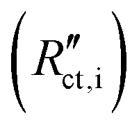 . The resulting circuit is shown in Fig. 10a. Please note that the electronic coupling capacitor Ci/e enters the ionic rail in front of the SEI bulk resistance. As a consequence, it is no longer possible to use the analytical solution of our transmission line model with four terminals. Supposed both charge transfer resistances are small compared to the ionic bulk resistance of the SEI RSEI we end up with the simple circuit shown in Fig. 10b: the bulk-type R|C element of the SEI is simply in series to a Warburg impedance in parallel to Ci/e. This means that the bulk of an SEI layer should be considered by a separate serial element rather than by combining it with the charge transfer resistance in a Randles circuit.
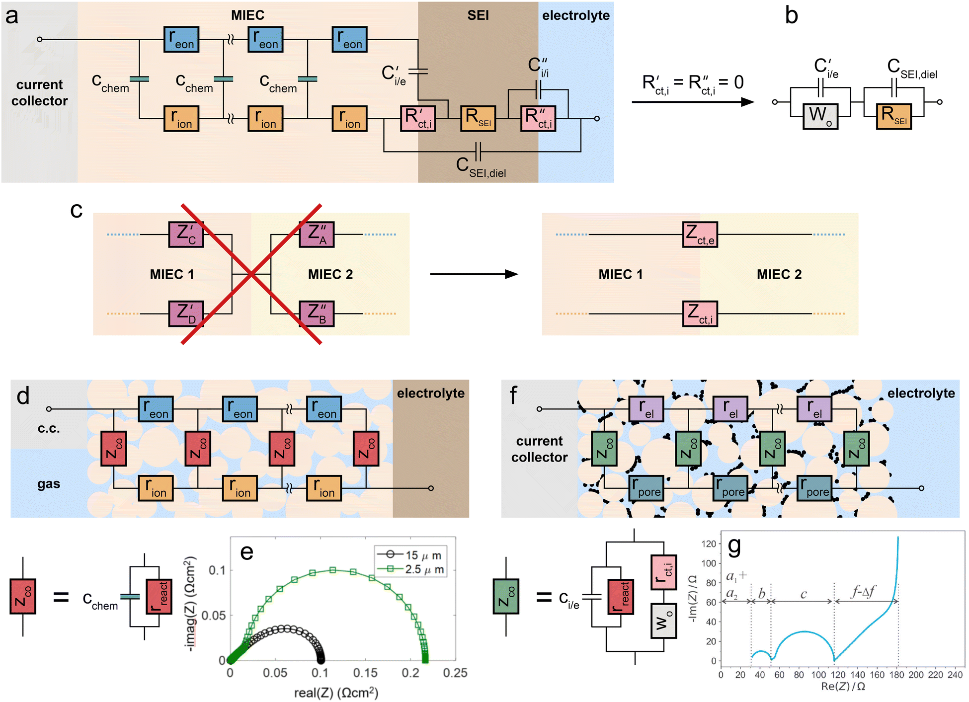 | ||
| Fig. 10 (a)–(d) Schematic transmission line for a porous solid oxide electrode. The element cchem is replaced by a general differential coupling impedance zco, which in this case corresponds to a simple rreact|cchem element. For simplicity, charge transfer resistances are neglected. (e) Simulated impedance spectra for porous SOFC electrodes of 2.5 μm and 15 μm thickness. Original image published in ref. 4 under a CC-BY 4.0 license. (f) Schematic transmission line for a porous battery electrode. For negligible reon, the coupling impedance zco corresponds to a Randles circuit, here with a finite side reaction resistance rreact (g) Simulated impedance spectrum for a de-Levie-type battery transmission line, similar to the circuit in (f). Reprinted with permission from ref. 2. | ||
Real SEI layers are chemically and geometrically complex and may consist of several phases.65,66 This causes a distribution of relaxation times, which might empirically be considered by using a constant phase element instead of the bulk capacitor CSEI,diel.67 In general, such constant phase elements are often more adequate than capacitors for describing interfacial capacitances and may thus be used at all terminals instead of ideal capacitors. However, the physical reasons causing such “non-ideal capacitors” are often unknown. The situation becomes even more complex when the secondary phase itself is also a mixed conductor. Then two transmission lines have to be combined in series, with both resistive rails transmitting into the second phase, possibly bridged by two charge transfer impedances, see Fig. 10c. Most importantly, it is not possible to simply add the two individual transmission line impedances, and thus also analytical solutions are usually no longer possible.
Porous electrodes
The second group of non-idealities frequently met in solid oxide cells and batteries are porous electrodes. Interestingly, extensions of the one-dimensional transmission line model for these two types of porous electrodes are rather different.In solid oxide cells, porous MIEC gas diffusion electrodes are quite common on the oxygen side, the pores being filled with the gaseous phase, thus enabling the coupling oxygen exchange reaction along the entire MIEC material. The complex tortuous conduction pathways along the thickness coordinate (distance from the electrolyte) are modelled by dividing the ionic/electronic conductivities by a microstructural factor M, given by σeff = σbulk/M. Additionally, the coupling between ionic and electronic current can be much more complex than the mere chemical capacitance, since coupling fluxes between the two rails are also possible via the oxygen exchange reaction at the surface. Therefore, instead of differential cchem elements, differential coupling elements zco are used, see Fig. 10d. Such a circuit is often called a de Levie model.68 The coupling impedances zco can often be approximated by rreact|cchem elements, with rreact corresponding to the oxygen exchange reaction at the MIEC surface (cf.Fig. 6c). For the rather common case of sufficiently thick and good electron conducting electrodes, this results in a Gerischer-type impedance69 shown by the black spectrum in Fig. 10e, given by the equation
 | (27) |
 and τ = RreactCchem. Finite electrode thickness, interfacial resistances4 and gas diffusion limitations70,71 make impedance models of real-world electrodes even more complex.
In batteries based on liquid electrolytes, on the other hand, porous electrodes are filled with electrolyte, leading to a strongly enhanced area of the electrode/electrolyte interface. Furthermore, carbon black is commonly added to the porous electrode to minimise the electronic contact resistance between the active material (MIEC) particles, as shown in Fig. 10f. Thus, the conduction pathways and overpotentials are more complex and consideration of ion transport in the electrolyte (in pores) causes an additional transmission line, with rel representing the incremental effective electronic resistance of the electrode and rpore being the incremental resistance of ion transport through the electrolyte-filled pores, both along the thickness coordinate. In this case, the coupling impedance zco describes the coupling of electronic charge carriers in the MIEC to ions in the electrolyte. This coupling includes interfacial charge transfer and ambipolar diffusion through the MIEC particles. For the typical case that the MIEC is predominantly electron conducting, zco takes the form of a Randles circuit (Fig. 10f).2 Since the Wo element corresponds to a simplified transmission line itself (Fig. 2c), the circuit shown in Fig. 10f can be considered as the MIEC's bulk transmission line nested into the structural transmission line of the porous electrode. In the corresponding impedance spectrum (Fig. 10g), arc b is due to the MIEC/current collector impedance, which is neglected in the circuit displayed here. Arc c is a convoluted feature with contributions primarily from rpore (electrolyte conduction in pores) and rct|ci/e elements, whereas the feature f is the Warburg impedance in Randles’ circuit that models the ambipolar Li diffusion within the particles. Again, real world electrodes are even more complex due to mobility of the PF6− anions, which causes concentration polarisation in the liquid electrolyte,2 SEI formation, or non-uniform distributions of particle shapes and sizes.
Multiple charge carriers
Materials that have more than two charge carriers can still be described by an extended transmission-line model with one rail for each carrier and coupling by chemical capacitors for each species.72 Typical examples here are proton conducting oxides that contain protons, oxygen vacancies and electrons as mobile species,73 as well as multi-ion liquid electrolytes.72 The treatment of such materials becomes tremendously more complex, because multiple ambipolar diffusion coefficients come into play. In solid proton conductors, for example, the H2O molecule, the H atom and the O atom can all diffuse as neutral species, each with a different diffusion coefficient. Additionally, boundary conditions for each carrier must be specified. The impedance of such circuits requires numerical computation.Conclusions
The impedance of dense mixed ionic and electronic conductors (MIECs) is consistently described by a one-dimensional transmission line consisting of two resistive rails for ion and electron conduction, coupled by chemical capacitors. The resulting circuit is physically exact in terms of the Nernst–Planck equation and provides a highly intuitive and practical approach to understanding and evaluating the impedance responses of various MIEC devices. Four terminal R|C elements at the rail ends allow a tailored adaptation of the general transmission line to specific measurement configurations, which can be classified as symmetrical (e.g. setups for the characterisation of bulk properties), SOFC-type and battery-type. For deciding which terminal elements should be used and which one may be negligible, it is helpful to distinguish between two types of terminals: those where the corresponding charge carrier can simply pass to the contact by charge transfer and those where an electrochemical reaction is required to couple a blocked resistance rail to the still transmissive rail.Besides providing a universal starting point for the intuitive derivation of tailored, physically exact impedance models, the general transmission line provides several key insights:
(1) Equivalent circuit elements can either represent charge transport resistances or the rates of electrochemical reactions that couple electron and ion currents. This difference becomes graphically clear in a transmission line picture.
(2) The general transmission line is consistent with the classical finite Warburg elements Ws and Wo, which are derived from Fick's law of diffusion for negligible electrical potential gradients (σion ≪ σeon) under the corresponding boundary conditions.
(3) The resistive and capacitive circuit elements in the corresponding transmission lines of the Warburg elements can be identified as the incremental ionic resistance rion (Rion = ∑rion) and the incremental chemical capacitance cchem (Cchem = ∑cchem), respectively.
(4) The general transmission line provides an extension of these Warburg elements for MIECs with finite σeon (e.g. σion ≈ σeon) by considering a resistive rail for electronic transport with Reon = ∑reon.
(5) For measurements with symmetrical contacts that are completely blocking towards one charge carrier and fully transmissive towards the other, the impedance spectrum consists of two arcs, with a shape and size reflecting the relevance of ionic and electronic contributions.
(6) For an additional charge transfer resistance, the spectrum consists of three arcs, all of which can be fitted to a single transmission line circuit.
(7) The impedance response of a bulk-limited SOFC electrode with negligible surface resistances corresponds to a finite-length Warburg element (Ws), due to the symmetry of the Ws transmission line. For a non-negligible surface exchange resistance, neither Ws nor a serial connection of Ws and the surface exchange resistance appropriately describe the electrode impedance. Only the full transmission line allows a physically meaningful interpretation of the corresponding impedance spectra.
(8) An SOFC electrode can be transformed into an oxygen-ion battery electrode by blocking the oxygen exchange reaction at the MIEC surface.
(9) Randles’ circuit is a special case of the general asymmetric transmission line model, where σion ≪ σeon, and only one interfacial capacitance Ci/e at the MIEC|electrolyte interface. Thus, for the given boundary conditions, Randles’ circuit can be considered as physically exact in terms of the Nernst–Planck equation.
(10) Within Randles’ circuit, a finite side-reaction resistance Rsr can be placed in parallel to Ci/e to consider, for example, electrolyte oxidation or reactions with impurities in the electrolyte, while remaining fully consistent with the general transmission line.
(11) A finite electronic resistance hinders the application of a simple Randles’ circuit and causes a serial high-frequency offset Rbulk = (Rion−1 + Reon−1)−1 in the impedance spectrum.
Author contributions
A. E. Bumberger: conceptualisation (equal), investigation, writing – original draft, A. Nenning: writing – review & editing, J. Fleig: supervision, conceptualisation (equal), writing – review & editing.Conflicts of interest
There are no conflicts to declare.Acknowledgements
The authors acknowledge TU Wien Bibliothek for financial support through its Open Access Funding Program.References
- A. Flura, C. Nicollet, S. Fourcade, V. Vibhu, A. Rougier, J. M. Bassat and J. C. Grenier, Electrochim. Acta, 2015, 174, 1030–1040 CrossRef CAS.
- J. Moskon and M. Gaberscek, J. Power Sources Adv., 2021, 7, 100047 CrossRef CAS.
- J. Moskon, J. Zuntar, S. D. Talian, R. Dominko and M. Gaberscek, J. Electrochem. Soc., 2020, 167, 140539 CrossRef CAS.
- A. Nenning, C. Bischof, J. Fleig, M. Bram and A. K. Opitz, Energies, 2020, 13, 987 CrossRef CAS.
- A. E. Bumberger, C. Boehme, J. S. Ring, S. Raznjevic, Z. Zhang, M. Kubicek and J. Fleig, Chem. Mater., 2023, 35, 5135–5149 CrossRef CAS PubMed.
- A. E. Bumberger, S. Raznjevic, Z. L. Zhang, G. Friedbacher and J. Fleig, J. Mater. Chem. A, 2023, 11, 24072–24088 RSC.
- A. E. Bumberger, C. Steinbach, J. Ring and J. Fleig, Chem. Mater., 2022, 34, 10548–10560 CrossRef CAS PubMed.
- A. Schmid, G. M. Rupp and J. Fleig, Phys. Chem. Chem. Phys., 2018, 20, 12016–12026 RSC.
- W. Lai and S. M. Haile, J. Am. Ceram. Soc., 2005, 88, 2979–2997 CrossRef CAS.
- H. Rickert, Electrochemistry of Solids, Springer, Berlin, Heidelberg, 1st edn, 1982 Search PubMed.
- C. Ho, I. D. Raistrick and R. A. Huggins, J. Electrochem. Soc., 1980, 127, 343–350 CrossRef CAS.
- J. R. Macdonald, J. Chem. Phys., 1973, 58, 4982–5001 CrossRef CAS.
- J. Jamnik and J. Maier, J. Electrochem. Soc., 1999, 146, 4183–4188 CrossRef CAS.
- J. Jamnik and J. Maier, Phys. Chem. Chem. Phys., 2001, 3, 1668–1678 RSC.
- J. Jamnik, J. Maier and S. Pejovnik, Electrochim. Acta, 1999, 44, 4139–4145 CrossRef CAS.
- M. Adamic, S. D. Talian, A. R. Sinigoj, I. Humar, J. Moskon and M. Gaberscek, J. Electrochem. Soc., 2019, 166, A5045–A5053 CrossRef CAS.
- A. Schmid, M. Krammer and J. Fleig, Adv. Energy Mater., 2023, 13, 2203789 CrossRef CAS.
- J. Maier, Z. Naturforsch. B, 2020, 75, 15–22 CrossRef CAS.
- V. F. Lvovich, Impedance Spectroscopy Applications to Electrochemical and Dielectric Phenomena, John Wiley & Sons, Ltd, New Jersey, 2012 Search PubMed.
- M. Gerstl, G. Friedbacher, F. Kubel, H. Hutter and J. Fleig, Phys. Chem. Chem. Phys., 2013, 15, 1097–1107 RSC.
- J. Jiang, W. Shen and J. L. Hertz, Solid State Ionics, 2013, 249, 139–143 CrossRef.
- I. Kosacki, C. M. Rouleau, P. F. Becher, J. Bentley and D. H. Lowndes, Solid State Ionics, 2005, 176, 1319–1326 CrossRef CAS.
- C. Peters, A. Weber, B. Butz, D. Gerthsen and E. Ivers-Tiffee, J. Am. Ceram. Soc., 2009, 92, 2017–2024 CrossRef CAS.
- Y. Hamon, A. Douard, F. Sabary, C. Marcel, P. Vinatier, B. Pecquenard and A. Levasseur, Solid State Ionics, 2006, 177, 257–261 CrossRef CAS.
- E. Navickas, M. Gerstl, G. Friedbacher, F. Kubel and J. Fleig, Solid State Ionics, 2012, 211, 58–64 CrossRef CAS PubMed.
- C. Ahamer, A. K. Opitz, G. M. Rupp and J. Fleig, J. Electrochem. Soc., 2017, 164, F790–F803 CrossRef CAS.
- S. Smetaczek, A. Limbeck, V. Zeller, J. Ring, S. Ganschow, D. Rettenwander and J. Fleig, Mater. Adv., 2022, 3, 8760–8770 RSC.
- X. Vendrell and A. R. West, J. Electrochem. Soc., 2018, 165, F966–F975 CrossRef CAS.
- L. Le Van-Jodin, F. Ducroquet, F. Sabary and I. Chevalier, Solid State Ionics, 2013, 253, 151–156 CrossRef CAS.
- H. Buschmann, J. Dölle, S. Berendts, A. Kuhn, P. Bottke, M. Wilkening, P. Heitjans, A. Senyshyn, H. Ehrenberg, A. Lotnyk, V. Duppel, L. Kienle and J. Janek, Phys. Chem. Chem. Phys., 2011, 13, 21658–21659 RSC.
- J. Fleig, Solid State Ionics, 2002, 150, 181–193 CrossRef CAS.
- M. Gerstl, E. Navickas, G. Friedbacher, F. Kubel, M. Ahrens and J. Fleig, Solid State Ionics, 2011, 185, 32–41 CrossRef CAS PubMed.
- X. Guo and R. Waser, Prog. Mater. Sci., 2006, 51, 151–210 CrossRef CAS.
- R. Amin and Y. M. Chiang, J. Electrochem. Soc., 2016, 163, X7 CrossRef CAS.
- J. Fleig, A. Schmid, G. M. Rupp, C. Slouka, E. Navickas, L. Andrejs, H. Hutter, L. Volgger and A. Nenning, Acta Chim. Slov., 2016, 63, 509–518 CAS.
- C. B. Zhu, C. Wu, C. C. Chen, P. Kopold, P. A. van Aken, J. Maier and Y. Yu, Chem. Mater., 2017, 29, 5207–5215 CrossRef CAS.
- M. Morgenbesser, S. Taibl, M. Kubicek, A. Schmid, A. Viernstein, N. Bodenmüller, C. Herzig, F. Baiutti, J. D. Sirvent, M. O. Liedke, M. Butterling, A. Wagner, W. Artner, A. Limbeck, A. Tarancon and J. Fleig, Nanoscale Adv., 2021, 3, 6114–6127 RSC.
- M. Siebenhofer, F. Baiutti, J. D. Sirvent, T. M. Huber, A. Viernstein, S. Smetaczek, C. Herzig, M. O. Liedke, M. Butterling, A. Wagner, E. Hirschmann, A. Limbeck, A. Tarancon, J. Fleig and M. Kubicek, J. Eur. Ceram. Soc., 2022, 42, 1510–1521 CrossRef CAS.
- G. M. Rupp, M. Glowacki and J. Fleig, J. Electrochem. Soc., 2016, 163, F1189–F1197 CrossRef CAS.
- M. Siebenhofer, U. Haselmann, A. Nenning, G. Friedbacher, A. E. Bumberger, S. Wurster, W. Artner, H. Hutter, Z. L. Zhang, J. Fleig and M. Kubicek, J. Electrochem. Soc., 2023, 170, 014501 CrossRef CAS.
- M. Siebenhofer, T. M. Huber, G. Friedbacher, W. Artner, J. Fleig and M. Kubicek, J. Mater. Chem. A, 2020, 8, 7968–7979 RSC.
- B. A. Boukamp and H. J. M. Bouwmeester, Solid State Ionics, 2003, 157, 29–33 CrossRef CAS.
- A. Nenning, L. Volgger, E. Miller, L. V. Mogni, S. Barnett and J. Fleig, J. Electrochem. Soc., 2017, 164, F364–F371 CrossRef CAS.
- J. Ring, A. Nenning and J. Fleig, J. Electrochem. Soc., 2023, 170, 050530 CrossRef CAS.
- T. Shimonosono, Y. Hirata, Y. Ehira, S. Sameshima, T. Horita and H. Yokokawa, Solid State Ionics, 2004, 174, 27–33 CrossRef CAS.
- T. Broux, B. Fleutot, R. David, A. Brull, P. Veber, F. Fauth, M. Courty, L. Croguennec and C. Masquelier, Chem. Mater., 2018, 30, 358–365 CrossRef CAS.
- R. Amin, P. Balaya and J. Maier, Electrochem. Solid-State Lett., 2007, 10, A13–A16 CrossRef CAS.
- J. S. Lee and H. I. Yoo, Solid State Ionics, 1994, 68, 139–149 CrossRef CAS.
- C. Riedl, M. Siebenhofer, A. Nenning, A. Schmid, M. Weiss, C. Rameshan, A. Limbeck, M. Kubicek, A. K. Opitz and J. Fleig, J. Mater. Chem. A, 2022, 10, 14838–14848 RSC.
- J. Fleig, H. R. Kim, J. Jamnik and J. Maier, Fuel Cells, 2008, 8, 330–337 CrossRef CAS.
- M. Krammer, A. Schmid, A. Nenning, A. E. Bumberger, M. Siebenhofer, C. Herzig, A. Limbeck, C. Rameshan, M. Kubicek and J. Fleig, ACS Appl. Mater. Interfaces, 2023, 8076–8092 CrossRef CAS PubMed.
- M. Krammer, A. Schmid, M. Siebenhofer, A. E. Bumberger, C. Herzig, A. Limbeck, M. Kubicek and J. Fleig, ACS Appl. Energy Mater., 2022, 8324–8335 CrossRef CAS PubMed.
- F. S. Baumann, J. Fleig, H. U. Habermeier and J. Maier, Solid State Ionics, 2006, 177, 1071–1081 CrossRef CAS.
- M. Krammer, A. Schmid, M. Kubicek and J. Fleig, J. Power Sources, 2023, 577, 233167 CrossRef CAS.
- R. Amin, J. Maier, P. Balaya, D. P. Chen and C. T. Lin, Solid State Ionics, 2008, 179, 1683–1687 CrossRef CAS.
- J. Illig, M. Ender, T. Chrobak, J. P. Schmidt, D. Klotz and E. Ivers-Tiffee, J. Electrochem. Soc., 2012, 159, A952–A960 CrossRef CAS.
- J. C. Jiang, W. Shi, J. M. Zheng, P. J. Zuo, J. Xiao, X. L. Chen, W. Xu and J. G. Zhang, J. Electrochem. Soc., 2014, 161, A336–A341 CrossRef CAS.
- Y. D. Liu and J. Xie, J. Electrochem. Soc., 2015, 162, A2208–A2217 CrossRef CAS.
- K. Tang, X. Q. Yu, J. P. Sun, H. Li and X. J. Huang, Electrochim. Acta, 2011, 56, 4869–4875 CrossRef CAS.
- L. Li, Y. L. Xu, R. Chang, C. Wang, S. N. He and X. D. Ding, Energy Storage Mater., 2021, 37, 325–335 CrossRef.
- J. K. Eckhardt, P. J. Klar, J. D. Janek and C. Heiliger, ACS Appl. Mater. Interfaces, 2022, 14, 35545–35554 CrossRef CAS PubMed.
- J. Fleig and J. Maier, Electrochim. Acta, 1996, 41, 1003–1009 CrossRef CAS.
- J. Fleig and J. Maier, Solid State Ionics, 1996, 85, 17–24 CrossRef CAS.
- J. Fleig and J. Maier, J. Electroceram., 1997, 1, 73–89 CrossRef CAS.
- X. B. Cheng, R. Zhang, C. Z. Zhao, F. Wei, J. G. Zhang and Q. Zhang, Adv. Sci., 2016, 3, 1500213 CrossRef PubMed.
- Y. L. Chu, Y. B. Shen, F. Guo, X. Zhao, Q. Y. Dong, Q. Y. Zhang, W. Li, H. Chen, Z. J. Luo and L. W. Chen, Electrochem. Energy Rev., 2020, 3, 187–219 CrossRef.
- M. Steinhauer, S. Risse, N. Wagner and K. A. Friedrich, Electrochim. Acta, 2017, 228, 652–658 CrossRef CAS.
- O. E. Barcia, E. D’Elia, I. Frateur, O. R. Mattos, N. Pébère and B. Tribollet, Electrochim. Acta, 2002, 47, 2109–2116 CrossRef CAS.
- S. B. Adler, J. A. Lane and B. C. H. Steele, J. Electrochem. Soc., 1996, 143, 3554–3564 CrossRef CAS.
- S. Dierickx, T. Mundloch, A. Weber and E. Ivers-Tiffée, J. Power Sources, 2019, 435, 69–82 CrossRef.
- A. Flura, C. Nicollet, S. Fourcade, V. Vibhu, A. Rougier, J. M. Bassat and J. C. Grenier, Electrochim. Acta, 2015, 174, 1030–1040 CrossRef CAS.
- Z. Siroma, N. Fujiwara, S. Yamazaki, M. Asahi, T. Nagai and T. Ioroi, J. Electroanal. Chem., 2020, 878, 114622 CrossRef CAS.
- D. Poetzsch, R. Merkle and J. Maier, J. Power Sources, 2013, 242, 784–789 CrossRef CAS.
Footnote |
| † Electronic supplementary information (ESI) available. See DOI: https://doi.org/10.1039/d4cp00975d |
| This journal is © the Owner Societies 2024 |