Unraveling gelation kinetics, arrested dynamics and relaxation phenomena in filamentous colloids by photon correlation imaging

Abstract

The fundamental understanding of the gelation kinetics, stress relaxation and temporal evolution in colloidal filamentous gels is central to many aspects of soft and biological matter, yet a complete description of the inherent complex dynamics of these systems is still missing. By means of photon correlation imaging (PCI), we studied the gelation of amyloid fibril solutions, chosen as a model filamentous colloid with immediate significance to biology and nanotechnology, upon passage of ions through a semi-permeable membrane. We observed a linear-in-time evolution of the gelation front and rich rearrangement dynamics of the gels, the magnitude and the spatial propagation of which depend on how effectively electrostatic interactions are screened by different ionic strengths. Our analysis confirms the pivotal role of salt concentration in tuning the properties of amyloid gels, and suggests potential routes for explaining the physical mechanisms behind the linear advance of the salt ions.

---

1 Introduction

Gels are, for decades, under the spotlight of both fundamental research and application advances.^1–5 Their widespread use is favoured by the possibility of gelating a wide range of colloidal systems through diverse mechanisms. At the same time, sustainability concerns call for narrowing the virtually infinite range of synthesis routes, towards ecological sources and processes.⁶ In this scenario, food sources can play a huge role, as they are both renewable and largely available.⁷ Polysaccharides and proteins can, in fact, gel through modification of three main key parameters: temperature, pH or ionic strength of the initial dispersions.⁸ For instance, one can think about the percolation of TEMPO-oxidized CNFs (cellulose nanofibrils), upon decrease of pH towards the pK_a of the carboxylic surface groups,⁹ the network formation of starch upon cooling¹⁰ and the morphological transitions (both at the intra- and inter-chain levels) of κ-carrageenan upon the addition of specific ions.¹¹

Among food gels, the ones made out of proteins are being increasingly studied in many research fields. One class of proteinaceous aggregates of high relevance is amyloid fibrils;¹² synthesized in vitro from food sources, amyloid fibrils can form liquid-crystalline phases¹³ and can be used to build innovative materials with multiple functionalities (such as heavy metal removal from water,¹⁴ iron fortification¹⁵ and sensing¹⁶). Amyloid fibrils can also originate in vivo from proteins or peptides that play a physiological role;¹⁷ an enhanced understanding of this amyloidogenesis process would enable better treatment protocols for neuro-degenerative diseases correlated with the presence of amyloid-plaques (such as Alzheimer's and Parkinson's).¹⁸ In both the described scenarios, advances in understanding of how amyloid fibrils interact and entangle are pivotal for further steps in research and application.

An excellent model food protein for synthesising and studying amyloid fibrils is β-lactoglobulin (βLG), which constitutes the main protein fraction of whey (a valuable side-stream of cheese production). High temperature and low pH conditions drive the unfolding and hydrolysis of βLG monomers; the formed shortened peptides, then, self-assemble into amyloid fibrils.^19,20 The resulting elongated colloidal objects (few nm in thickness and up to several μm in contour length) have a semi-flexible nature and an IsoElectric Point (IEP) close to 5.²¹ At the synthesis pH (which usually ranges between 2 and 3) βLG amyloid fibrils are, therefore, positively charged and form a viscous suspension stabilized by electrostatic repulsion. Gelation is promoted by supplying ions, the role of which is to screen the surface charges and to consequently decrease the repulsive forces among the considered polyelectrolytes.²² The shear elastic modulus (G) of amyloid gels was found to scale with the concentration of fibrils (c) and with the ionic strength (I), respectively, as G ∼ c^2.2 and G ∼ I^4.4. The strong dependence of the shear modulus on I could be rationalised through DLVO theory: the mechanical strength of the gel is related to the probability (p) of transforming entanglement points into long-lived physical cross-links (p ∼ I^4.1, where the scaling exponent is very close to 4.4).²³ Another recent study showed the possibility of correlating the plateau value of the intermediate scattering function of amyloid gels (extracted through a non-ergodic treatment of dynamic light scattering data) to their mesh size (ξ_m).²⁴ However, despite the mentioned major advances in the understanding of the static properties of the already-formed amyloid gels, many unanswered questions on their dynamics still remain. How amyloid gels form and how frozen-in stresses relax in time are still open points in the current literature.

By means of photon correlation imaging (PCI), a light scattering technique able to follow dynamic phenomena with both spatial and temporal resolution, we followed the gelation of two amyloid fibril suspensions upon the supply of monovalent ions (Na⁺ and Cl⁻) from salt reservoirs at different ionic strengths. We found that the gelation front, in both cases, evolved linearly in time (y ∼ t): such observation is in marked contrast with the expected diffusive behaviour . This phenomenon was already observed in the case of a polysaccharide hydrogel;²⁵ its physical explanation is hypothesized to be related to a combination of the Donnan effect and osmotic pressure unbalances. Besides the interesting behaviour of the gelation front, we found out that the two gels formed at different ionic strengths exhibited sudden rearrangement phenomena, the behaviour of which was a function of the salt concentration. In more detail, higher salt concentrations are associated with decorrelation events which are lower in magnitude, but more homogeneous in space (as a consequence of the higher elastic modulus of the material).

The collected pieces of evidence and the performed analysis shed light on the complex physical mechanisms that underlie amyloid gel formation, with valuable benefits for enhancing the synthesis of innovative materials in vitro. In fact, as amyloid fibrils are highly functional in a wide range of applications, a deeper understanding of the gelation kinetics of amyloid solutions would allow scientists and industrial researchers to optimize the synthesis parameters of materials based on amyloid arrested states.

2 Materials and methods

2.1 βLG monomer purification

βLG monomers were purified from WPI (whey protein isolate, Fonterra, New Zealand) according to an already published protocol.²⁶ To avoid the presence of residual salts during fibrillization, βLG monomers were further purified through the following steps. 10 g of purified powder was dissolved in 90 g of Milli-Q water at neutral pH and, after complete dissolution, the pH of the solution was adjusted to 1.9 with a concentrated HCl solution (VWR Switzerland). Nylon syringe filters (FilterBio®, ∅ 0.22 μm) were used to remove the eventual aggregates and to pour the solution into dialysis membranes (Spectra/Por® Standard RC Tubing, MWCO 6–8 kDa, D = 32 mm, Spectrum Laboratories Inc.), which were afterwards closed with clips and put in 5 L of deionized water at pH 3. The equilibration bath was changed six further times with 5 L of Milli-Q water at neutral pH; the filled membranes were left in each bath for a minimum time of 6 hours. The used succession of the pH values of the equilibration baths (3 for the first, and neutral for the six following ones) enabled keeping the pH of the βLG monomer solutions to values lower than the IEP of the protein, and allowed avoiding therefore undesired aggregation phenomena. After purification, the pH of the βLG monomer solution was adjusted to 2 with a concentrated HCl solution. The mass fraction of monomers was determined through gravimetric analysis, by taking aliquots of 400 μL and letting them evaporate in a 60 °C oven; as a consequence of dilution over the dialysis process, the weight fraction was determined to be 3.8 wt%. 120 mL of the solution were kept for preparing amyloid fibrils, while the rest was freeze-dried for further usage.

2.2 βLG amyloid fibril synthesis and characterization

108 mL of Milli-Q at pH 2 were used to dilute the above-mentioned 120 mL of the βLG monomer solution, to reach a final weight fraction of 2 wt%. The resulting solution was transferred to a Schott bottle and heated up at 90 °C for 5 hours, while stirring with a 5 × ∅ 0.75 cm Teflon-coated magnetic stirrer. The solution was stirred at 100 RPM for the first 1 h and 20 min of the process; successively, the Schott bottle was manually shaken to break the gel layer at the interface, and the stirring speed was increased to 120 RPM until the end of the process. After 5 hours, the system was quenched with ice. The resulting solution of amyloid fibrils was centrifuged in 50 mL tubes to remove macroscopic aggregates, two times at 5000 g for 10 minutes, and one time at 20 000 g for 15 minutes. The solution was stored in a 200 mL plastic beaker and, before further usage, was newly centrifuged in plastic vials at 10 000 g for 10 minutes (to remove the aggregates formed over the storing process). The experiments presented in this work were performed out of a single batch of βLG amyloid fibrils, prepared as outlined above.

The formed amyloid fibrils were characterized through AFM (atomic force microscopy) imaging. For the preparation of the AFM sample, a 0.01 wt% solution of βLG amyloid fibrils was prepared through dilution with Milli-Q at pH 2. Afterwards, 20 μL of the mentioned dispersion was deposited on the surface of freshly cleaved mica and subsequently rinsed with 1 mL of pH 2 Milli-Q, after incubation for 2 minutes. Gentle drying with airflow completed the sample preparation, which was afterwards characterized under ambient conditions with a Dimension FastScan Bio scanning probe microscope (Bruker, USA), using a commercial cantilever (Bruker, USA) working in the tapping mode.

The amyloid fibrils, together with a statistical analysis performed using the open-source software FiberApp,²⁷ are shown in Fig. S1 (ESI†).

2.3 βLG amyloid fibril gel preparation

As stated in the introductory section, this work focuses on perfusion-induced amyloid fibril gels. The gels were prepared in PS cuvettes (with external dimensions of 12 × 12 × 45  mm and an optical path of 10 mm) with 4 optical windows (Kartell, Italy), by pouring 2 mL of 2 wt% amyloid fibril solutions. Successively, the piston of a 2.5 mL syringe (Terumo Europe) was removed and the remaining plastic part was transversely cut with a scissor, with the aim of creating a cylindrical reservoir for the salt solution. One side of the cylindrical reservoir was sealed (using Parafilm®) with a dialysis membrane, obtained from one side of a dialysis tube (MWCO 12 kDa, D-9777, lot. 10B049777, Sigma-Aldrich Chemie GmbH) which had previously been washed with deionized water. 1.5 mL of pH 2 NaCl solutions (at either 150 or 300 mM, depending on the performed experiment) was poured into the sealed cylindrical reservoir, which had previously been put in contact with the βLG amyloid fibril dispersion in the plastic cuvette. In this way, the salt could pass through the dialysis membrane into the amyloid fibril dispersion. Before carrying out the experiments, the density of the used solutions (300 mM NaCl at pH 2, 150 mM NaCl at pH 2 and 2 wt% amyloid fibrils in pH 2 Milli-Q water) was determined by measuring the weight of volumetric aliquots. This analysis confirmed the higher density of the amyloid dispersion; considering that such a solution was placed in the bottom part of the cuvette, there were no inverse density gradients which could enhance the diffusion of salt through the creation of convective rolls.²⁵ The final system, before starting the measurement, was sealed with Parafilm® to avoid evaporation. We tested the appropriateness and robustness of the used perfusion setup by measuring and analysing potential samples of interest at different ionic strengths: the considerations that emerged from such a preliminary phase, and that lead to the choice of the two above-mentioned ionic strengths for the reservoir, are reported in Section 2 of the ESI.† The characterisation studies of the samples at either high or low salt molarity were then performed as single experiments.

To show the gel nature of the prepared samples, three systems prepared with a 300 mM NaCl solution were characterized through oscillatory sweeps. A AR 2000 stress-controlled rheometer (TA Instruments) was used in a plate–plate (40 mm) geometry: after setting the temperature control to 20 °C, the upper reservoir containing the salt solution was removed from the cuvettes and ∼500 μL of the formed gel was sampled with the use of a plastic spatula and deposited on the rheometer. After reaching the geometry gap of 400 μm, a solvent trap was put on the rheometer and oscillatory sweep measurements at 1% strain between 0.0628 and 157.8 rad s⁻¹ were performed. The results of the statistical analysis of the three independent measurements are presented in Fig. S3 (ESI†).

2.4 Photon correlation imaging (PCI)

Before detailing the experimental setup and the image analysis approach used in our study, we find it beneficial to share key information on the used technique.

Photon correlation imaging measures the intensity time-correlation function of the light scattered by the studied sample, with both temporal and spatial resolution; this enables probing the local dynamics within the scattering volume, with an eye open to temporally heterogeneous events.

In PCI experiments, a speckled image of the scattering volume at a given angle θ is formed on a multipixel detector. The imaging optics consist of a lens and a diaphragm placed at the focal distance, which select a precise scattering wave vector q, and cause in parallel the “speckled” appearance of the collected images. The intensity at each given point on the image plane originates from the interference of the light scattered by a finite-size region in the sample plane. Quantitatively, the detected speckle patterns, made by N pixels, are first divided into regions of interest (ROIs). Then, the space-time degree of correlation c_I(r,t,τ) is computed as:

The notation 〈⋯〉_r indicates the ensemble spatial average of a ROI centered in r. To minimize the influence of imaging/analysis procedures,²⁸ it is often useful to define a normalized version of the space–time degree of correlation ĉ_I(r,t,τ) by introducing c_I(r,t,0), the relative variance of the intensity measured in r at time t.²⁵ The normalized space–time degree of correlation will be referred to, hereinafter, as correlation index:

The multi-speckle and the near-field scattering natures of the technique allow it to keep a parametric dependence on time from the beginning of the experiments (t) and on the position r, respectively. One key consequence of this is the possibility of catching both temporally and spatially heterogeneous phenomena. In more detail, decorrelation bursts can be highlighted by means of the so-called “dynamic activity maps” (DAMs),²⁹ without losing the possibility of averaging ĉ_I(r,t,τ) over time to locally quantify the dynamics of the colloidal objects through the intensity correlation function g⁽²⁾(r,t,τ) − 1 = 〈ĉ_I(r,t,τ)〉_δt. The time-span δt, over which the correlation index is averaged, has to be shorter than the characteristic timescale of the evolution of the system. This is favoured, in practice, by the multi-speckle nature of the technique that promotes a faster averaging compared to other correlation techniques that employ single-speckle detectors (like the majority of dynamic light scattering setups).

PCI belongs to a broader family of recently established optical techniques, based on near field scattering (NFS).^30,31 Another powerful technique in the mentioned family is DDM (differential dynamic microscopy),³² which blends scattering and imaging by analysing data acquired using a microscope in the Fourier domain. Although the mentioned technique is suitable for a broad range of purposes, that range from the characterisation of polymeric systems³³ to the one of biological media,³⁴ we chose to use PCI as the detection angle and optics allowed us the choice of a precise wave-vector, diversely from the case of DDM where the collected images result from the convolution of information at different characteristic length-scales; this focuses the analysis on a single length-scale, compatible with the microscopic features of the system.

For details about the PCI equipment used in this study, we refer to a recently published article where the same experimental configuration was used.³⁵ The cuvette containing the amyloid fibril solution was inserted into the thermostatic holder of the setup, which was connected to a recirculating bath. The temperature was kept constant at 25 °C over the course of the entire experiment, with oscillations that did not exceed ≈ 0.1 °C. The sample was illuminated by a vertical laser sheet (λ = 532  nm, Ventus Diode-Pumped Solid State) and the scattering volume was imaged on a CMOS camera (Hamamatsu Orca Flash 4.0, 2048 × 2048 square pixels of size 6.5 μm, 16-bit depth), by an achromatic doublet set at θ = 90° with respect to the illumination plane. The mutual distances between the optical elements in the imaging segment set the magnification close to 1 (with a magnified pixel having a size of 6.7 μm). The diaphragm placed in the focus of the imaging lens precisely selects a specific scattering wave vector q = (4π/λ)n sin(θ/2) ≈ 22 μm⁻¹, and sets the speckle size to ∼13 × 13 μm, which corresponds to 2 × 2 pixels. The choice of q was operated on the base of a two-fold set of criteria. From a geometrical perspective, a measuring angle of θ = 90° is optimal for the used cuvettes, which have a squared section with four clear sides. In parallel, the length-scale associated with the probed q-vector (δ = 2π/q ∼ 300 nm) is compatible with the characterisation of the microscopic dynamics of the network forming units, as it is only a few times larger than the estimated mesh size of the amyloid fibril network (which will be computed later on in the manuscript).

Images of 2048 (V) × 1000 (H) pixels (successively cropped to 2000 × 900 pixels to exclude areas that were external to the cuvettes) were acquired with the above-mentioned CMOS camera, with an exposure time of 10 ms and a frame rate of 1/60 fps. The imaged area is shown in Fig. 1, with a color-code that evolves from wine purple to yellow as the distance from the dialysis membrane increases; such a colour scheme will be thoroughly used in the upcoming sections. More precisely, the imaged area starts roughly 4 mm below the dialysis membrane, to let the gelation front properly adapt from the cylindrical reservoir to the squared cross-section of the cuvette. The speckled appearance of the images, once corrected for noise and non uniform illumination, is shown in Fig. S4 in the ESI† and in the magnification in Fig. 1.

Fig. 1 Schematic of the cuvette where the gelation is induced. The gelation front is considered to start from the dialysis membrane (dashed black line in the proximity of the syringe), and to evolve in the positive y direction. The 0 value of the y axis is taken in correspondence to the beginning of the imaged area: a progressive increment of the distance from the 0 value is color-coded with a shift from wine purple to bright yellow (as represented on the y axis itself). The probed area has a size of around 13.4 × 6 mm and creates on the CMOS camera an image with a speckled appearance (as shown by magnification in the figure). The acquired images, after post-processing (as outlined in Fig. S4 and Sub-section 4.1 in the ESI†), were divided into regions of interest (ROIs) and analysed through the computation of the correlation index (defined by Eq. 2). As an example, the right hand side of the figure shows ĉ_I(r,t = 300 min, τ = 1 min) for the sample at a higher molarity, after the images were divided into ROIs each containing 20 × 20 pixels. The values of the correlation index (from 0 to 1) are associated with a color scale (from red to blue) that symbolizes the evolution of the amyloid fibril suspension from a viscous dispersion (ĉ_I ∼ 0) to a gel (ĉ_I ∼ 1).

The correlation index ĉ_I(r,t,τ) was then computed for each ROI using a custom-made code running on MATLAB®.

3 Results & discussion

3.1 General considerations on sample gelation

The 2 wt% amyloid fibril suspensions were gelled with two NaCl salt solutions at pH 2, having a molarity of 300 mM and 150 mM, respectively. In the following, we will refer to the first mentioned sample as the one with a higher salt molarity (HSM), and to the second as the one with a lower salt molarity (LSM). Due to the finite size of the reservoir, for both samples, the concentration of the salt lowers as the ions pass through the semi-permeable membrane. Considering the ratio between the volumes of the βLG and the salt solutions (respectively, 2 mL and 1.5 mL), a homogeneous diffusion of the salt would lead to final concentrations of ∼ 129 mM (for HSM) and of ∼ 65 mM (for LSM). According to previous studies,^22,23 the mentioned values of ionic strength transform 2 wt% βLG amyloid fibril solutions into gels. To explain the different dynamics of, respectively, the solution and gelled states, and to understand the consequent changes in the values of the computed values of ĉ_I, it is beneficial to dig into the motion of semi-flexible polymers. Before doing so, it is useful to extract further static parameters of the network of interest. The cubic lattice (l_c) model gives an estimation of the mesh size (ξ_m) of the network at the studied concentration (c_p ∼ 2 wt% ∼ 20 mg mL⁻¹) of protein; assuming the conversion of monomers into amyloids (ϕ) to be roughly 40%, a radius of the fibers (a) of 1.5 nm (Fig. S1, ESI†) and a fiber density (ρ) of 1300 mg mL⁻¹ we obtain:²⁴

It can be noted that the length-scale probed by the optical apparatus (δ = 2π/q ∼ 300 nm) is five times larger than the estimated mesh size, and is therefore sensitive to the characteristic dynamics of multiple filaments. Before the solution transforms into a gel, the single fibrils can bend, rotate or translate. All the mentioned typologies of motion are constrained by the surrounding objects, due to the presence of entanglement points;³⁶ however, the labile nature of such entanglements allows motions whose magnitude makes the correlation index fully decay. When the local concentration of salt gets higher, the probability of transforming entanglements into long-lived crosslinks increases, due to the concomitant screening of electrostatic repulsive forces.²³ As a consequence, the rotational and translational degrees of freedom are further hindered and the fibrils only express bending fluctuations,³⁷ whose magnitude is small compared to the probed length-scale. As a consequence, close-to-one values of ĉ_I are observed. For the statements above to be met, we base the computation of the correlation index on a time delay value (τ) equal to 1 min. This value is aligned with the aim we wanted to achieve, as it lies between the characteristic relaxation times of the fibrillar network constituting units (in the order of 10⁻⁴–10⁻² s, at the probed wavevector) and the one of the formed gels (in the order of 10¹–10³ s); the reader can obtain more insights on the two mentioned time-scales, in Section 5 of the ESI.† The value of the chosen lag-time (1 min) drives the observation of full decorrelation (ĉ_I ∼ 0) in areas where the gel has not formed yet, and correlation (ĉ_I ∼ 1) in areas where the gel has already formed.

For the HSM sample (whose gel state was confirmed by rheology experiments, Fig. S3, ESI†), there was actually the potential risk of the salt driving local agglomeration, and increasing therefore the turbidity of the sample; in the phase diagram shown by Bolisetty and co-workers, gels approach the state of translucent solutions, as the molarity increases.²² However, it has to be considered that the mentioned phase diagram refers to materials prepared by mixing. In Fig. S6 (ESI†) it is possible to appreciate the transparency of the HSM gel prepared by perfusion: we attribute the difference to the lower quantity of agglomerates created with a gentle supply of salt, compared to the rapid local increase of salt molarity that accompanies the mixing method.

Another indication of the limited agglomeration of amyloid fibrils, over the duration of the whole experiment, can be appreciated by analysing the temporal evolution of the scattered intensity of both HSM and LSM samples. Since, during the gelation kinetics, the scattered intensity and the correlation index are expected to depend only on the vertical position y, the speckle pattern images were each subdivided into 40 ROIs with a height of 50 pixels and laterally extending over the whole width of the investigated sample region (900 pixels). Each ROI contains therefore about 11 250 speckles, a value which was found to yield a good vertical resolution with a limited statistical noise in the correlation function.

The time evolution of the scattered intensities (〈I_p(t)〉_r/〈I_p(0)〉_r) for ROIs located at the bottom part of the cuvettes, for both HSM and LSM samples, are presented in Fig. S7 (ESI†); the reader is referred to Section 7 of the ESI,† for a detailed analysis on the influence of background contributions and on the relationship between the evolution of the scattered intensity and the one of the correlation index. Here, we focus on the main piece of information: the scattered intensity, for both samples, increases by a factor slightly larger than 2, which is moderate compared to the ones detected in other food gels. In fact, in alginate dispersions, it was possible to observe an increase of the scattered intensity by a factor of 20, upon diffusion of divalent cations.²⁵ The observed difference can be attributed to the different gelation mechanisms of the two considered bio-polymer dispersions. In the case of βLG amyloid fibrils, the colloidal units undergo limited changes as a consequence of gelation: the effect of the diffusing ions is to convert labile entanglements into long-lived cross-links, and therefore the scattering pattern that arises from intra-colloidal properties changes only slightly. In the case of alginate, instead, the observed drastic change in scattered intensity is related to profound modifications of the morphology of the network-forming units.

3.2 Evolution of the gelation front

Fig. 2 shows the behaviour of the gelation front for both HSM and LSM, studied upon the division of the images (background-corrected as explained in Section 4 of the ESI†) in ROIs with the same properties as the ones used for analysing the temporal change in scattered intensity (height = 50 pixels, width = 900 pixels). This choice takes into account the expected horizontal spatial homogeneity of the studied system, and has the further advantage of enabling the description of the studied area (at a fixed t) with an array of ĉ_I values, rather than with a matrix. As a consequence, it is possible to plot the values of ĉ_I(y,t,τ = 1 min) as a color map, with y being the distance from the first ROI and t being the time from the beginning of the observation (Fig. 2A and B): a colour shift from red (ĉ_I ∼ 0) to blue (ĉ_I ∼ 1) suggests a slowing down of the dynamics. For HSM (panel A), after a time-scale of 1000 minutes, the whole imaged area gets fully arrested. In the case of LSM (panel B), double the time is needed to gel the same area. It can be noticed that, in panel A, the upper 3 cm of the imaged area are already in an arrested state at the beginning of the observation, while this does not hold true for panel B. Some considerations on this point are shared in Fig. S8 and Section 8 of the ESI.†

Fig. 2 Color maps representing the behaviour of the correlation index calculated at a fixed τ = 1 min, as a function of the distance from the first ROI (y axis) and of the time from the beginning of the observation (x axis), for HSM (panel A) and LSM (panel B), respectively. For this analysis, the images were divided into ROIs with a height of 50 pixels and a lateral extension of 900 pixels (that encompasses the entire width of the imaged area). In each panel, the linear-in-time evolution of the gelation front is highlighted by black dashed lines, which are a guide to the eye.

As the gelation front evolves progressively, the higher the distance of the ROIs from the membrane, the higher the characteristic time at which the dynamics shift from totally decorrelated (red colour) to arrested (dark blue color). If a characteristic value of ĉ_I is considered as a benchmark for gelation, it is possible to compute the gelation time (t_g, calculated as the instant when ĉ_I gets larger than 0.4) as a function of the distance from the first ROI. In both panels it can be appreciated how t_g scales linearly with time (dashed black lines), with a speed of v = 1.47 × 10⁻² mm min⁻¹ and v = 7.77 × 10⁻³ mm min⁻¹ for HSM and LSM, respectively. The mentioned values of the speed were extracted through linear fits of t_gvs. y. Approaching the bottom of the cell, the front velocity increases: this acceleration is more evident in LSM and is symbolized by a change in slope of the orange-to-green transition region.

As already pointed out, βLG gelation is caused by the local increase of ionic strength, which lowers the electrostatic repulsion between fibrils and allows the formation of physical bonds. Assuming that gelation takes place instantaneously when the local ion concentration c(y,t) reaches a threshold value c*, we can suppose that the gel front kinetics resembles the one of the aforementioned threshold concentration. A simple diffusive behaviour of salt ions, which predicts an increase of the gel thickness as the square root of time 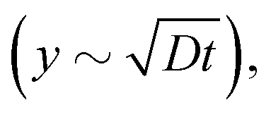is clearly not able to account for the initial constant velocity. The observed linear evolution might indicate the existence of a net force that causes an advective behaviour. Indeed, we may consider the solution of the generalized 1D diffusion equation ∂c(y,t)/∂t = −v∂c(y,t)/∂y + D∂²c(y,t)/∂y² for the ion concentration c(y,t), under zero-flux boundary conditions. If we set a particular threshold concentration c = c* for gelation, the solution of the differential equation predicts an initial linear advance of c* with time, followed by a speed up close to the boundary caused by the impossibility of the ions to migrate beyond the impermeable wall, as can be shown analytically in the case of simple diffusion close to a wall.³⁸

Further hints to address the puzzling linear-in-time evolution of the gelation front can be taken from previous studies on food gels. Secchi and co-workers, while studying the evolution of the gelation front of alginate gels, also noted a linear advance.²⁵ Alginate has a negative surface charge at pH 7 and its gelation is driven by providing specific, divalent ions (Ca²⁺), which act through the egg-box model (aggregation of single chains). Therefore, the morphology of the network forming units changes because of gelation, by forming thicker strands that afterwards build the network up. On the side of this, the divalent cations that promote gelation get locally trapped; the behaviour of the ions therefore cannot be described with a simple diffusion-advection model, as also a negative reaction term (that accounts for the transition of the ions from a free to a bound state) is necessary.^39,40 In the case of this polysaccharide, the observed linear advance was attributed to a depletion layer in front of the gel, deduced from a minimum of the scattered intensity; the existence of such a layer was explained through a combination of the spatial advance of the gel with a concomitant shrinkage, the consequence of which was the creation of an alginate-free zone. The inverted density profile presumably caused natural micro-convective rolls, which are known to influence the diffusive behaviour by speeding up its dynamics. The mentioned mechanisms, in our case, may hardly account for the observed phenomenon: in fact, shrinkage phenomena in βLG amyloid fibril gels are very limited (as confirmed in Fig. S6, ESI†). As an example of this statement, we observed that gels keep being transparent and without observable macroscopic shrinkage even weeks after they have been prepared with the protocol mentioned in this manuscript (data not shown). Moreover, the gelation mechanism of βLG amyloid fibril gels is strikingly different from that in the case of alginate: the conversion of entanglements into cross-links does not alter significantly the morphological properties of the network-forming units, and is promoted by non-specific salt ions that do not get locally trapped. The ions only have a charge screening role, and can therefore diffuse further: consequently, the description of their behaviour does not need to take into account a negative reaction term.

A hypothesis that better aligns with the observed gelation dynamics of amyloid gels relies on the electrostatic effects. In a former study, the ionic strength of a pectin dispersion was increased through dissolution of monovalent ions (which are non-specific for pectin, and therefore did not induce gelation); afterwards, a structural arrest was induced by perfusion of divalent cations.⁴¹ In such an experimental configuration the gelation front was observed to advance diffusively, in contrast to the linear advance observed in the case of alginate (where the ionic strength of the medium had not been previously increased). The authors hypothesized that the Donnan effect might be thought as responsible for what was observed.⁴² In more detail, in systems where confinement or energetic contributions influence the entropy-driven spatial configuration of charged colloids, the electroneutrality of the whole system can be kept with a concomitant generation of an electrostatic potential (named the Donnan potential). This further energetic term has an additional influence on the spatial configuration of the charged species present in the system. This is the case, as an example, if two compartments containing ionic species are separated by a selectively permeable membrane.^43,44 Further pieces of evidence of the mentioned phenomenon can be observed in the barometric density profile of charged colloids, where an electrostatic potential difference was both theoretically hypothesized and measured.^45–47 In our case (a filamentous colloidal gel), the crosslinks bind the chains together, hindering their free diffusion and then in fact confining them. The whole gel region behaves therefore as an “extended osmotic membrane” for the βLG fibrils, and since βLG is charged, this membrane is subjected to a Donnan equilibrium. In a nutshell, this means that, because one species (the protein) cannot diffuse through the membrane (in this case, escape from the gel), while the product of the concentrations of the mobile ions will be the same in and out of the gel, the concentration of each ionic species may instead be different. In practice, this means that, during the gelation kinetics, the concentration of ions with a sign opposite to that of βLG (which are also those responsible for chain aggregation) is higher just outside the gel moving boundary, leading to a faster aggregation of those chains that are close to this interface. We assumed that this introduces a time-linear propagation, rather than a diffusive, term in the kinetic equations because it is in fact equivalent to an electric field (related to the Donnan potential) “pulling” the gel.

On the side of the electric force that stems from the Donnan potential, changes in the electrostatic screening length in the polyelectrolyte system as the salt advances might further encourage the described phenomenon.⁴⁸ When a polyelectrolyte solution evolves from an entangled state to a physically cross-linked one, the osmotic pressure exerted by the charged amyloid fibrils varies; in particular the reduction in the osmotic pressure associated with the sol–gel transition (arising from the newly forming intermolecular contacts) is expected to lead an acceleration to the migration of the ions and thus of the gelation front.

All these effects are thought to contribute to the observed behavior of the moving gel front. Despite the fact that our explanation is just qualitative, it can be used as a base for performing a further quantitative evaluation; as this is far from being trivial, it would require further extensive experiments on different systems.

3.3 Gel restructuring events

We focus now on analysing in more detail the behaviour of the normalized correlation index, for HSM and LSM.

In Fig. 3A, the behaviour of ĉ_I at τ = 1 min for HSM, at different distances from the first ROI (same color-code as in Fig. 1), can be appreciated. Despite this being a different plot format than the one in Fig. 2A, more information can actually be visualized, especially in terms of decorrelation events. The four arrows in panel A of Fig. 3 refer to the other panels, with a color-scheme that relates the colours of the arrows to the ones of the frames of the panels. The mentioned panels consist of dynamic activity maps, where the spatial distribution of the correlation index is represented by a color map. In order to better identify the temporal heterogeneities within the sample in both the horizontal and vertical directions, we performed the DAM analysis upon redefining the ROIs as squares of 20 × 20 pixels.

After 50 minutes from the beginning of the observation (B), only the top part of the area is arrested (dark blue color), while the rest of the solution exhibits a totally decorrelated state (at the shortest computable delay, τ = 1 min). As the gelation front proceeds, progressively more ROIs get arrested: panel C shows a situation where half of the area is arrested, and the other half still shows fully expressed decorrelation dynamics. After a time-scale of 1000 minutes (panel D), the entire examined area is arrested. However, biological and colloidal gels are often not truly fully arrested once formed. As a function of the underlying aggregation kinetics, stresses might freeze inside the structure, and subsequently release through time-intermittent rearrangement phenomena.^25,49–52 A piece of evidence that supports the given picture is presented in panels E, F and G, where the evolution of the most pronounced rearrangement event over the entire measurement is represented. The occurrence of the mentioned event is indicated with the grey arrow in Fig. 3A. At 3856 minutes the structure is fully arrested (E); then, a rearrangement event that spans the entire illuminated area happens and causes the correlation index to drop to lower values (F). One minute later, the structure is again fully arrested in the new, less stressed configuration assumed after the rearrangement (G). The moderate magnitude of the re-configuration event is appreciable by the fact that ĉ_I locally drops, at maximum, to values close to 0.5.

Fig. 3 (A) Normalized correlation index (ĉ_I) of HSM, computed at a constant delay time τ = 1 min, as a function of the time from the beginning of the observation (t). The different curves, in accordance with the color-scheme in Fig. 1, represent ROIs at different distances from the membrane. The coloured arrows refer to the other panels that compose the figure, in accordance with the colour of the frames by which they are surrounded. (B) Dynamic activity map (DAM) at t_B = 50 min. (C) DAM at t_C = 400 min. (D) The fully arrested state of the solution, which has transformed into a gel (t_D = 1000 min). (E–G) DAM sequence that shows the occurrence of a rearrangement event of moderate magnitude. The three DAMs are at t_E,F,G = 3856, 3857 and 3858 min, respectively.

We now shift our focus on the sample gelled with a lower ionic strength (Fig. 4). The arrows in Fig. 4A refer to the other panels, in accordance with the used color code. As already pointed out for the HSM sample, reconfiguration events mostly occur after the full evolution of the gelation front. After the gelation front had encompassed the entire probed area, within the first 2500 min of observation (panels B, C and D), the behaviour of the correlation index from ∼ 2500 min onward is characterized by a high number of sudden drops, of which the largest is displayed in the sequence (E–G). A fully arrested structure (E) suddenly exhibits correlation drops that propagate over the entire upper part of the cuvette (F), with the successive acquisition of a new arrested state over the timescale of few minutes (G). The first point of comparison between the mentioned event and the one of the HSM sample (discussed above) regards their magnitude and spatial propagation. While, in the case of HSM, ĉ_I dropped to minimum values of ∼ 0.5 in the whole imaged area, in LSM the correlation index drops to 0 in some areas. The second point lies, instead, in the time needed for the system to again reach high correlation. While, in the case of the HSM sample, 1 minute was sufficient to bring ĉ_I back to close-to-one values, the same statement does not hold true for the LSM sample. In the latter, more than 5 minutes are needed for ĉ_I to rise to pre-rearrangements values.

Fig. 4 (A) Normalized correlation index (ĉ_I) of LSM, computed at a constant delay time τ = 1 min, as a function of the time from the beginning of the observation (t). The different curves, in accordance with the color-scheme in Fig. 1, represent ROIs at different distances from the membrane. (B) Dynamic activity map (DAM) at t_B = 500 min. (C) Further advance of the gelation front (t_C = 1500 min). In the time span between B and C, at ∼ 800 min there is a major decorrelation event, which is further discussed in section 9 of the ESI.† (D) DAM at t_D = 2500 min. (E–G) DAM sequence that shows the occurrence of a rearrangement event in the upper part of the cuvette (t_E = 3720 min, t_F = 3721 min and t_G = 3730 min).

More details on the differences between the HSM and LSM samples can be gained by a quantitative, statistical analysis of the decorrelation events, which is presented in Fig. 5. To perform this analysis, the images were divided into ROIs with dimensions of 50 × 50 pixels, which were then used to compute the value of the correlation index ĉ_I(r,t,τ). This resulted in 40 lines of ROIs (at different y coordinates), each comprising 18 ROIs that covered the full width of the imaged area. For each sample, among the 40 lines of ROIs, we choose to analyze the ones at three different heights: line 1 (y ∼ 0 mm), line 20 (y ∼ 6.7 mm) and line 40 (y ∼ 13.4 mm). In order to decouple the kinetics of the gelation of the samples from the decorrelation events, for each value of t between 3000 and 4000 min, the 18 ĉ_I values (computed at τ = 1 min) in each line were averaged; then, the so-obtained x-averaged correlation indices were smoothed using a moving average filter based on the MATLAB® smooth function (method: rloess, span: 0.2), to obtain the quantity 〈ĉ_I〉_smooth. For each t and each line, the obtained quantity was then subtracted from the 18 local values of the correlation indices computed from the 50 × 50 pixels ROIs. In this way, for each horizontal line that was considered, it was possible to obtain the deviation of 18000 values of the local correlation index from their x-averaged, time-smoothed counterpart (considering the entire time window of 1000 min).

Fig. 5 Statistical analysis of the decorrelation events, for both the HSM (panels A and B) and LSM samples (panels C and D). Panels A and C represent the probability density function of the difference between the ĉ_I values and 〈ĉ_I〉_smooth in the considered ROIs, as discussed in the text. Panels B and D represent the time-dependence of the just mentioned quantity, for specific ROIs located at three different heights in the sample (y ∼ 0 mm, wine purple circles; y ∼ 6.7 mm, brown squares; and y ∼ 13.4 mm, light yellow triangles).

The probability density function (pdf) of the quantity ĉ_I − 〈ĉ_I〉_smooth is presented in Fig. 5A and C, respectively, for the HSM and the LSM samples. Different colours and shapes of the symbols are associated with the different y coordinates, as highlighted in the legends. Panels B and D represent instead the time evolution of ĉ_I − 〈ĉ_I〉_smooth for an arbitrary ROI in each considered line (in fact, plotting the data of all the 18 ROIs would have made the reading and interpretation of the graph less straightforward); the used colour code is the same as in panels A and C, and they also, respectively, refer to HSM and LSM.

In panels A and C, for each plotted pdf, the data that respected the condition ĉ_I − 〈ĉ_I〉_smooth > 0 were fitted using Gaussian functions with a null mean (μ = 0), with the aim of extracting the standard deviation (σ, considered as a fitting parameter) of the distributions. In fact, when no decorrelation events are present, the correlation index is expected to perform Gaussian fluctuations around an average value.⁵³ The values of σ extracted from the fitting are reported in the legends of panels A and C. This procedure allowed us to establish a consistent and robust definition of the de-correlation events; we considered as such all data-points that fulfilled the condition ĉ_I − 〈ĉ_I〉_smooth < −5σ, and we highlighted them in all the panels of Fig. 5 using a red-pink colour.

The first point to be noted is that the two samples are characterised by different values of σ; in other words, the correlation index of the LSM samples performs larger excursions around its time-smoothed and x-averaged counterpart. In fact, the σ values for the HSM sample are roughly half of those of the LSM sample. The second point to be highlighted, which also emerged in the previous analysis, is the different absolute magnitude of the decorrelation events. In panel C, we can appreciate the decorrelation events at ĉ_I − 〈ĉ_I〉_smooth values that are smaller than −0.6; on the other hand, in panel A no decorrelation events are smaller than −0.35. This can be explained by the difference in ionic strength. On the one hand, in HSM the gelation is promoted faster than in LSM; consequently, frozen in stresses are more likely to be present in the initial configuration. On the other hand, the factor 2 in the ratio between the final ionic strengths translates into a factor larger than 10 in the ratio between the probabilities of the transforming entanglements into physical cross-links (p_HSM/p_LSM ∼ (I_HSM/I_LSM)^4.1 ∼ 16).²³ This determines, in the HSM case, a higher number of constraints for a single fibril; a more formal way to express such a concept is by affirming that the cross-linking length approaches the entanglement one.⁵⁴ In such a state, the relaxation of stresses is made more difficult by the high number of long-lived cross-links; heterogeneous phenomena are expected, as a consequence, to be not pronounced in magnitude. The third point to be discussed, is actually related to the just-mentioned fact that higher molarities convert more effectively entanglements into cross-links, and therefore enhance the elastic modulus of the material (G ∼ I^4.4). In HSM, the higher elastic modulus allows a better propagation of the relaxation events, with the consequence that they have only small degrees of spatial heterogeneity. This is confirmed by the fact that, in panel A, the decorrelation events related to the three different heights overlap well; panel B confirms this view, as only the top panel (related to y ∼ 0) shows a slightly larger number of decorrelation events. This last observation can also be attributed to the fact that the gel formed at y ∼ 0 mm is “older” than the one formed at y ∼ 6.7 mm and y ∼ 13.4 mm, and is characterised by a lower value of σ (and therefore by a lower threshold for defining an event as a decorrelation one). On the other hand, the lower G value of the LSM sample makes the decorrelation events more heterogeneous in space. From panel C, it can be appreciated that the decorrelation event population is dominated by circles (y ∼ 0 mm), followed by squares (y ∼ 6.7 mm) and triangles (y ∼ 13.4 mm). This can be even better appreciated in panel D, where the top sub-panel (y ∼ 0 mm) is the one that presents larger amounts of decorrelation events, with a larger magnitude. The middle sub-panel (y ∼ 6.7 mm) shows fewer decorrelation events, with lower absolute magnitude, and this statement holds even truer for the bottom sub-panel (y ∼ 13.4 mm); this suggests that the region affected by the reconfigurations in the LSM gel is the most aged one, where the gel first forms, in contrast to what happens in alginate gels where the decorrelation always starts from the sol–gel interface.²⁵ The hypothesised picture, in which a lower salt concentration is less effective in driving the conversion of entanglements into long-lived cross-links, is confirmed also by the aforementioned time to reach again high correlation, that is longer in the LSM sample.

The same considerations shared above hold true also for the rearrangement events occurring during the gelation (Fig. S9 and Section 9 therein, ESI†), although it is not possible to reach clear conclusions on the spatial propagation of the stress-release events (due to the limited size of the region where the gel had already formed). In more detail, a higher ionic strength is correlated with less enhanced drops of the correlation index and to a faster regain of pre-reconfiguration values.

4 Conclusions

The performed analysis gives precious hints on the dynamic properties of amyloid fibril gels, prepared by ion permeation into entangled networks. The first, pivotal point to be highlighted is the observed linearity of the advance of the gelation front; although such a phenomenon had already been observed in other systems, the discrepancy with an expected diffusive behaviour is, at first, confusing. We shared the hypothesis that the observed behaviour might be related to the Donnan effect and to electrostatic screening heterogeneity; we are currently working on developing a physical model to describe the mentioned observation. Another relevant point to be highlighted is the role of the salt concentration in tuning both the velocity of the gelation front and the magnitude of rearrangement events. A higher salt concentration not only allows the gelation front to proceed faster, but also has a role in converting many entanglement points into physical cross-links. As a consequence, the gel has a more fixed structure and is less sensitive to stress-releasing events, which happen locally but easily propagate to larger areas due to the high elastic modulus of the material. On the other hand, a lower salt concentration makes the gelation front evolve slower; the parallel, lower conversion of entanglements into cross-links allows wide and drastic reconfigurations both during gelation and after an arrested structure is formed. In the case of lower salt molarity, more time is needed for the normalised correlation index to rise back to pre-stress release events values and the reconfigurations are more heterogeneous in space (and mostly happening in the aged parts of the sample).

The highlighted phenomena might be a common feature to all those systems that form arrested structures because of the screening of electrostatic repulsive forces, and have therefore an ionic strength-dependent cross-link length. Particularly promising approaches to further investigate these systems would be to blend a microrheology analysis with time-cure superposition (TCS),⁵⁵ to extract the gel point and the critical scaling exponents of the systems.^56–58 However, care has to be taken, so that the surface chemistry and the size of the added tracers do not influence the extracted properties.^59,60 Another very interesting possibility, would be the analysis of rearrangement events or relaxation phenomena during shearing. Setups for performing scattering and microscopy experiments while shearing samples of interest have already been reported in the literature,⁶¹ and applied to model systems for extracting non-affine displacements with the help of a rigorous theoretical framework.^62,63

We believe that the shared observations and explanations widen the understanding of amyloid networks and set a more solid background for future studies and analyses.

Author contributions

The author contributions are listed in accordance with the guidelines from CRediT, for standardised contribution descriptions. Mattia Usuelli: conceptualization, data curation, formal analysis, investigation, methodology, software, visualization, and writing – original draft. Vincenzo Ruzzi: conceptualization, data curation, formal analysis, investigation, methodology, software, and writing – review and editing. Stefano Buzzaccaro: resources (design and construction of the PCI setup), conceptualization, methodology, supervision, and writing – review and editing. Gustav Nyström: conceptualization, methodology, supervision, and writing – review and editing. Roberto Piazza: conceptualization, funding acquisition, methodology, project administration, resources, supervision, and writing – review and editing. Raffaele Mezzenga: conceptualization, funding acquisition, methodology, project administration, resources, supervision, and writing – review and editing.

Conflicts of interest

There are no conflicts to declare.

Acknowledgements

We would like to thank Marco Campello for help in the acquisition of the PCI images and for interesting discussions, and Massimo Bagnani for help in the acquisition of the AFM images. V. R., S. B. and R. P. acknowledge funding from Ministero dell'Università e della Ricerca (PRIN Project 2017Z55KCW, “Soft Adaptive Networks”).

References

1. E. Zaccarelli, J. Phys.: Condens. Matter, 2007, 19, 323101.
2. D. Saha and S. Bhattacharya, J. Food Sci. Technol., 2010, 47, 587–597.
3. G. Tiwari, R. Tiwari, B. Sriwastawa, L. Bhati, S. Pandey, P. Pandey and S. K. Bannerjee, Int. J. Pharm. Invest., 2012, 2, 2–11.
4. S. Zhao, W. J. Malfait, N. Guerrero-Alburquerque, M. M. Koebel and G. Nyström, Angew. Chem., Int. Ed., 2018, 57, 7580–7608.
5. D. Arcos and M. Vallet-Reg, Acta Biomater., 2010, 6, 2874–2888.
6. J. D. Sachs, G. Schmidt-Traub, M. Mazzucato, D. Messner, N. Nakicenovic and J. Rockström, Nat. Sustainability, 2019, 2, 805–814.
7. Y. Cao and R. Mezzenga, Nat. Food, 2020, 1, 106–118.
8. A. H. Clark, in Food polymers, gels and colloids, ed. E. Dickinson, The Royal Society of Chemistry, Cambridge, 1991, ch. 26, pp. 322–338.
9. M. Arcari, R. Axelrod, J. Adamcik, S. Handschin, A. Sánchez-Ferrer, R. Mezzenga and G. Nyström, Nanoscale, 2020, 12, 11638–11646.
10. M. J. Miles, V. J. Morris, P. D. Orford and S. G. Ring, Carbohydr. Res., 1985, 135, 271–281.
11. M. Diener, J. Adamcik, A. Sánchez-Ferrer, F. Jaedig, L. Schefer and R. Mezzenga, Biomacromolecules, 2019, 20, 1731–1739.
12. Y. Cao and R. Mezzenga, Adv. Colloid Interface Sci., 2019, 269, 334–356.
13. G. Nyström, M. Arcari and R. Mezzenga, Nat. Nanotechnol., 2018, 13, 330–336.
14. S. Bolisetty and R. Mezzenga, Nat. Nanotechnol., 2016, 11, 365–371.
15. Y. Shen, L. Posavec, S. Bolisetty, F. M. Hilty, G. Nyström, J. Kohlbrecher, M. Hilbe, A. Rossi, J. Baumgartner and M. B. Zimmermann, et al. , Nat. Nanotechnol., 2017, 12, 642–647.
16. G. Nyström, M. P. Fernández-Ronco, S. Bolisetty, M. Mazzotti and R. Mezzenga, Adv. Mater., 2016, 28, 472–478.
17. M. G. Iadanza, M. P. Jackson, E. W. Hewitt, N. A. Ranson and S. E. Radford, Nat. Rev. Mol. Cell Biol., 2018, 19, 755–773.
18. P. C. Ke, R. Zhou, L. C. Serpell, R. Riek, T. P. Knowles, H. A. Lashuel, E. Gazit, I. W. Hamley, T. P. Davis and M. Fändrich, et al. , Chem. Soc. Rev., 2020, 49, 5473–5509.
19. J.-M. Jung, G. Savin, M. Pouzot, C. Schmitt and R. Mezzenga, Biomacromolecules, 2008, 9, 2477–2486.
20. J. Adamcik, J.-M. Jung, J. Flakowski, P. De Los Rios, G. Dietler and R. Mezzenga, Nat. Nanotechnol., 2010, 5, 423–428.
21. Y. Cao, S. Bolisetty, G. Wolfisberg, J. Adamcik and R. Mezzenga, Proc. Natl. Acad. Sci. U. S. A., 2019, 116, 4012–4017.
22. S. Bolisetty, L. Harnau, J.-M. Jung and R. Mezzenga, Biomacromolecules, 2012, 13, 3241–3252.
23. Y. Cao, S. Bolisetty, J. Adamcik and R. Mezzenga, Phys. Rev. Lett., 2018, 120, 158103.
24. M. Usuelli, Y. Cao, M. Bagnani, S. Handschin, G. Nyström and R. Mezzenga, Macromolecules, 2020, 53, 5950–5956.
25. E. Secchi, T. Roversi, S. Buzzaccaro, L. Piazza and R. Piazza, Soft Matter, 2013, 9, 3931–3944.
26. D. Vigolo, J. Zhao, S. Handschin, X. Cao, A. J. deMello and R. Mezzenga, Sci. Rep., 2017, 7, 1211.
27. I. Usov and R. Mezzenga, Macromolecules, 2015, 48, 1269–1280.
28. A. Duri, H. Bissig, V. Trappe and L. Cipelletti, Phys. Rev. E: Stat., Nonlinear, Soft Matter Phys., 2005, 72, 051401.
29. A. Duri, D. A. Sessoms, V. Trappe and L. Cipelletti, Phys. Rev. Lett., 2009, 102, 085702.
30. R. Cerbino and A. Vailati, Curr. Opin. Colloid Interface Sci., 2009, 14, 416–425.
31. R. Cerbino, Phys. Rev. A: At., Mol., Opt. Phys., 2007, 75, 053815.
32. R. Cerbino and V. Trappe, Phys. Rev. Lett., 2008, 100, 188102.
33. R. Cerbino, F. Giavazzi and M. E. Helgeson, J. Polym. Sci., 2022, 60, 1079–1089.
34. L. G. Wilson, V. A. Martinez, J. Schwarz-Linek, J. Tailleur, G. Bryant, P. Pusey and W. C. Poon, Phys. Rev. Lett., 2011, 106, 018101.
35. R. Piazza, M. Campello, S. Buzzaccaro and F. Sciortino, Macromolecules, 2021, 54, 3897–3906.
36. D. C. Morse, Phys. Rev. E: Stat., Nonlinear, Soft Matter Phys., 2001, 63, 031502.
37. K. Kroy and E. Frey, Phys. Rev. E: Stat., Nonlinear, Soft Matter Phys., 1997, 55, 3092–3101.
38. J. Crank, The Mathematics of Diffusion, Oxford university press, Oxford, 1979.
39. A. Mikkelsen and A. Elgsaeter, Biopolymers, 1995, 36, 17–41.
40. B. Thu, O. Gåserød, D. Paus, A. Mikkelsen, G. Skjåk-Bræk, R. Toffanin, F. Vittur and R. Rizzo, Biopolymers, 2000, 53, 60–71.
41. E. Secchi, F. Munarin, M. D. Alaimo, S. Bosisio, S. Buzzaccaro, G. Ciccarella, V. Vergaro, P. Petrini and R. Piazza, J. Phys.: Condens. Matter, 2014, 26, 464106.
42. F. G. Donnan, Chem. Rev., 1924, 1, 73–90.
43. A. Philipse and A. Vrij, J. Phys.: Condens. Matter, 2011, 23, 194106.
44. T.-Y. Wang, Y.-J. Sheng and H.-K. Tsao, J. Colloid Interface Sci., 2009, 340, 192–201.
45. R. van Roij, J. Phys.: Condens. Matter, 2003, 15, S3569–S3580.
46. A. P. Philipse, J. Phys.: Condens. Matter, 2004, 16, S4051–S4062.
47. M. Raşa and A. P. Philipse, Nature, 2004, 429, 857–860.
48. A. V. Dobrynin and M. Rubinstein, Prog. Polym. Sci., 2005, 30, 1049–1118.
49. O. Lieleg, J. Kayser, G. Brambilla, L. Cipelletti and A. R. Bausch, Nat. Mater., 2011, 10, 236–242.
50. Z. Filiberti, R. Piazza and S. Buzzaccaro, Phys. Rev. E, 2019, 100, 042607.
51. D. Larobina and L. Cipelletti, Soft Matter, 2013, 9, 10005–10015.
52. S. Buzzaccaro, A. F. Mollame and R. Piazza, Soft Matter, 2021, 17, 7623–7627.
53. P. N. Pusey and W. Van Megen, Phys. A, 1989, 157, 705–741.
54. C. P. Broedersz and F. C. MacKintosh, Rev. Mod. Phys., 2014, 86, 995.
55. D. Adolf and J. E. Martin, Macromolecules, 1990, 23, 3700–3704.
56. T. H. Larsen and E. M. Furst, Phys. Rev. Lett., 2008, 100, 146001.
57. M. D. Wehrman, S. Lindberg and K. M. Schultz, Soft Matter, 2016, 12, 6463–6472.
58. M. D. Wehrman, M. J. Milstrey, S. Lindberg and K. M. Schultz, Lab Chip, 2017, 17, 2085–2094.
59. I. Wong, M. Gardel, D. Reichman, E. R. Weeks, M. Valentine, A. Bausch and D. A. Weitz, Phys. Rev. Lett., 2004, 92, 178101.
60. M. Valentine, Z. Perlman, M. Gardel, J. H. Shin, P. Matsudaira, T. Mitchison and D. Weitz, Biophys. J., 2004, 86, 4004–4014.
61. S. Aime, L. Ramos, J.-M. Fromental, G. Prevot, R. Jelinek and L. Cipelletti, Rev. Sci. Instrum., 2016, 87, 123907.
62. S. Aime and L. Cipelletti, Soft Matter, 2019, 15, 200–212.
63. S. Aime and L. Cipelletti, Soft Matter, 2019, 15, 213–226.

---

Footnotes

† Electronic supplementary information (ESI) available. See DOI: https://doi.org/10.1039/d1sm01578h

‡ These authors contributed equally to this work.

---