 Open Access Article
Prediction of suitable catalysts for the OCM reaction by combining an evolutionary approach and machine learning†
Carlotta L. M.
von Meyenn
and
Stefan
Palkovits
 *
*
Institute of Technical and Macromolecular Chemistry, Worringerweg 2, 52074 Aachen, Germany. E-mail: stefan.palkovits@itmc.rwth-aachen.de; Fax: +49 241 80 22177; Tel: +49 241 80 20560
First published on 14th April 2023
Abstract
Catalytic systems are multidimensional and still difficult to interpret even by accomplished chemists. For years high throughput experimentation has been used to find new catalysts. We describe a method to use the concept of directed evolution to synthesize new catalysts for the oxidative coupling of methane in silico via a classical genetic algorithm. The evaluation of the novel catalysts is based on predicting the C2 yield with the help of a random forest algorithm.
1 Introduction
Catalyst design often takes a lot of resources and time. In the field of heterogeneous catalysis, the development strongly relies on chemists making educated guesses. Nevertheless, improving theoretical predictions, e.g. Density Functional Theory (DFT) analysis1,2 and high throughput experimentation3 are potent tools for the development of new catalysts. High throughput experimentation is still based on catalytic intuition of chemists or based on a vast amount of data.4 Machine learning is a powerful tool that has been widely used in various fields outside of chemistry, e.g. natural language processing.5 It could also be applied to improve the search for new catalysts.6 It is based on the statistical recognition of patterns in different datasets and extrapolating those patterns outside of the original dataset. Toyao et al. provide a good overview over the field7 from a chemistry centered viewpoint. The algorithm proposed here is used to find a connection between the suitability of a catalyst for the Oxidative Coupling of Methane (OCM) and the catalyst composition. It enables us to propose promising new catalysts for the OCM reaction only based on in silico experimentation. A genetic algorithm has been implemented. To ensure that this algorithm is easily adaptable for multiple datasets and reactions, it has been made as straightforward as possible. The dataset used for testing was initially collected by Zavyalova et al.8 In the publication of Takahashi et al.9 an alternative approach can be found how to treat this dataset in an even more data centered way.Oxidative coupling of methane (OCM)
The OCM is a possibility to synthesize C2 hydrocarbons presented by Keller et al. in 1982.10 The desired species by this reaction is ethylene, which is one of the most demanded basic petrochemicals and is mainly produced by steam cracking of hydrocarbons e.g. naphtha.11,12 The OCM converts methane to ethane and ethene at low pressures without using mediating syngas.13 Methane is usually combusted to generate heat and power. The OCM reaction gives the possibility to upgrade the abundance of methane into important bulk chemicals without expensive reforming steps.14 According to the proposed mechanism for most heterogeneous catalysts, methane is adsorbed on the surface of the catalyst and a methyl radical is generated. After it desorbs, it couples with another methyl radical to ethane. The ethane can be dehydrogenated to ethylene. Both steps produce water as a byproduct (eqn (1)). | (1) |
Parallel to the reactions shown above the oxidation of the present hydrocarbons to CO and CO2 takes place (eqn (2)) because at higher reaction temperatures (>873 K) CO2 is the thermodynamically favorable product.14
 | (2) |
Further insights into mechanistic aspects of the OCM reaction can also be found in recent literature.15 The study from Takahashi et al. also provides mechanistic insights from quantum chemical perspective.9 Over the years, a lot of possible catalysts for the OCM reaction have been synthesized and tested. However, only a few show the techno-economic targets of 35% C2 yield and 90% selectivity proposed in 1989.14
OCM dataset
The database published in 2011 by Zavyalova et al. consists of 1870 data points, which have been collected over 30 years. This database was further curated by Schmack et al. in 2019.16 It includes catalysts consisting of 68 different catalytic active elements (61 cations and seven anions). All elements are differentiated into active components (anions and cations), promoters (anions), and support material, usually in the form of oxides. Since the exact oxygen stoichiometry in the catalysts is unknown under OCM conditions, oxygen is not included in the database.8 Under the assumption that the yield and the selectivity depend only on the composition of the catalysts, a 68-dimensional dataset needs to be analyzed. The elemental composition acts as inputs into the algorithm (also called features), the C2 yield acts as output (also called target). If more factors e.g. reaction temperature and contact time, are included, the number of dimensions increases. Computational methods can make this easier and faster.Python
The language used for the evolutionary algorithm is Python. It has been chosen because it is open source, has an intuitive syntax and is applicable for a wide range of purposes. It is a reasonably fast to learn application development language and, therefore, suitable for non-expert programmers.17 Python has become a more and more popular language for chemistry-related applications and research.18–20 As a result, more packages designed for chemistry can be found.21–26 The implementation for this publication was done using Jupyter notebooks. Those give the possibility to mix Python code, markdown text, and LaTeX code, which makes it easy to comment on the code and makes it readable and accessible for people new to programming.27,28 They also have the advantage that graphs are shown directly. Since the machine learning step takes most of the computing time, comparing it with the other steps of the algorithm, especially the last point, is a considerable advantage.Random forest
Random Forest (RF) is a supervised learning algorithm. The algorithm can work with high dimensional data and does not need a specified model underlying the data, which makes it suitable for data from high throughput synthesis.Directed evolution
Directed evolution is a method developed to find new enzymes and binding proteins that has been developed by Frances H. Arnold, who was rewarded with the Nobel prize for Chemistry in 2018 for her work.29 It is based on the concept of emulating the natural evolution process with random mutations and selection. The same concept can also be applied to heterogeneous catalyst design. The evolutionary cycle consists of two main steps (a) diversification by random mutations or recombinations and (b) the selection of promising new variants.30 The power of directed evolution lies in a high mutation number per evolution cycle and a fast application of Darwin's concept of survival of the fittest by high throughput screening. By choosing fitness parameters that are aimed at a specific function, biochemists can design highly specialized enzymes or proteins without the exact knowledge of the structural and mechanistic information required for a rational design.31,322 Implementation
The implementation can be split into three categories: data preprocessing, training of the random forest and directed evolution. The data preprocessing has been implemented following the tutorial by S. Palkovits.28Random forest
The RF algorithm has been implemented following the tutorial by S. Palkovits28 with the major change of training the random forest regressor to predict the C2 yield of the reactions and not the selectivity of the products ethane and ethene. High selectivity is an essential property in deciding if a catalyst is well suited, but the accuracy of the predictions of the RF model is better for the yield than for the selectivity. The dataset is split into a train and test subset. The former is used to estimate the parameters of our model and the latter is used to evaluate the resulting model. The regression function is based on the constructing of decision trees and bagging (bootstrap aggregating). From the training dataset, B sub-datasets are sampled randomly with replacement. This ensures that the trained model is less sensitive to change in the dataset and is a method to reduce overfitting. For each of the B sub-datasets, a decision tree is constructed, reducing the loss as much as possible. The complexity of the tree is reduced via pruning the finished tree. An additional randomizing factor is introduced to reduce the correlation between the trees of each B sub-dataset. Each tree is built based on features selected randomly without replacement and gives one prediction function. All prediction functions are aggregated into one singular prediction function, which represents the response the trained algorithm gives for future predictions.10,33 Even though the support vector machine algorithm should be suited better for small datasets like the one used here, S. Palkovits showed that the results for the RF algorithm are slightly better than for the support vector machine.28 The ability of the RF to give a ranking of the features was not exploited in this study. To determine how well the regression of the random forest works, the coefficient of determination (also called R2 score) is used as a score. The closer to 1 the score is, the better the predictions of the model are. With this adjustment, the score on the training set is improved from 0.83 to 0.85 and the score on the test set from 0.29 to 0.44. However, this adjustment does not solve the problem of an overfitted RF function. Overfitting describes the phenomenon of fitting the model to the noise in the dataset instead of finding a general predictive rule, which is here indicated by the performance difference between training and test set. It occurs if the model is trained in a complex way so that its estimations have high variance but low bias, so a slight change in the training data can have a significant influence on the model. Bagging is one method to reduce overfitting because it decreases the variance of the model.34,35 The results on the catalyst data generated by the directed evolution can be compared with the results on the test set. The coefficient of determination is below 0.5 but the regression function is still useable to result in a clear trend that shows if the genetic algorithm works. Of course, a model with better scores would lead to improved results. However, because the implementation of the proposed evolutationary algorithm does not depend on a specific random forest model, our model can still be used to verify its functionality.Directed evolution
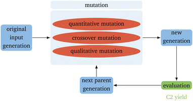
The basic flow of the directed evolution (Fig. 1) is straightforward and inspired by the methods used for the directed evolution of enzymes.30,31,36 It starts with several parents that already show some sort of the desired properties – in this case, a high yield for the OCM reaction. These are then mutated randomly to produce a new generation of catalysts. Those catalysts are evaluated regarding the desired property. This property describes the fitness of the catalyst. After evaluation, the best catalysts, according to our evaluation, are mutated again. In the proposed algorithm, the predicted C2 yield is used to describe the fitness. It is expected that the next generation always performs better than the generation before. The smaller the input generation (IG), the more generations are necessary to gain a good-performing catalyst. The smaller the next parent generation (PG) is, the higher the selective pressure.37 To keep the algorithm as simple as possible, the next PG has the same size as the original input parents. This leads only to a higher selective pressure if also the IG is small.To implement the genetic algorithm, three different mutation types were used, implemented separately, and then collected as a single evolution function: Qualitative Mutation, Quantitative Mutation and Crossover Mutation (Fig. 2). Implementing the mutation functions separately gives the possibility to use only one kind of mutation. This leads to easier troubleshooting. All mutations are based on a (pseudo) random number generator and have to lead to a new catalyst.
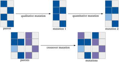 | ||
| Fig. 2 Schematic representation of the mutation mechanisms. The blue and violet represent metals and their lightness an arbitrary concentration. | ||
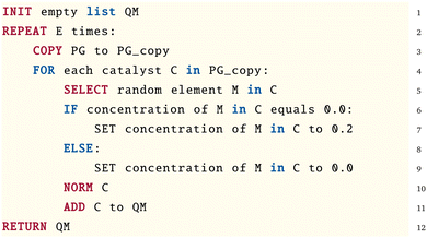
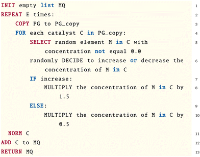
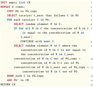
The qualitative mutation function (Alg. 1) switches an existing concentration in a catalyst to 0.0 or introduces a new element into the catalyst with a set concentration. The function is based on generating a list of the catalysts (binary generation) first.38 The new initial concentration in the used algorithm is 0.2. Since the RF algorithm has been trained only on the 68 elements already existing in the dataset, other elements can not be introduced. The quantitative mutation function (Alg. 2) changes the concentration of the elements already existing in the catalyst by randomly adding or subtracting half of the concentration of the chosen element. The concentration is randomly increased or diminished.38 The function for the crossover mutation function (Alg. 3) switches the concentration of one element of one catalyst with the one of another catalyst.38
Algorithm 1 Pseudo code of the qualitative mutation function.
Algorithm 2 Pseudo code of the quantitative mutation function.
Algorithm 3 Pseudo code of the crossover mutation function.
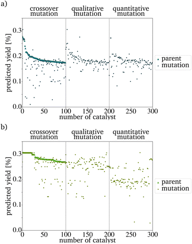
After all mutations are finished, the concentrations of each new catalyst are normalized to 1. Each mutation function has a different mutation power (MP). The qualitative mutation leads to consistently high variations and therefore has a strong MP. This is based on the huge influence a new or vanishing catalyst component has. Therefore the MP increases with the initial concentration of new elements (new_elements[new_elements_TF] = 0.2, Line 7 in Algorithm 1). The quantitative mutation has a smaller MP because only the amounts of the existing components are changed. The MP further decreases if the fraction by which the concentration is changed is lowered. The MP of the crossover mutation decreases over the generations. In early generations, the variance between the catalysts in the PG is high and therefore, the MP of the function is high. The later generations are more homogeneous than the original IG. The switching of the concentrations between two metals, therefore, has a much smaller influence and the MP is much smaller (Fig. 3). If the predicted yield (PY) of the catalysts is already similar, this leads to a further homogenization of the next generation. For each evolution cycle, every mutation is carried out E times for each catalyst on the parent input list with size P. The number of mutations generated in each generation equals the product of the number of parents P, the number of mutation functions, and the evolutionary factor E (eqn (3)). E represents the number of mutations generated by one mutation type per generation and catalyst.
| M = P·E·3 | (3) |
The evaluation criterium for the next PG is a high PY. The new PG has the same size as the original IG and is sorted by the PY. Since the RF predicts this yield, a better random forest model would lead to better predictions in the evolutionary algorithm. In the graphic representation, the sorting leads to a seemingly decreasing yield of the new parents. This effect is not based on the mutation algorithm itself but only on the preparation for an easy evaluation (Fig. 3). For every generation, a visual representation of the composition and PY of each generation and the overall development of the PYs has been implemented. By this, the development of the PY of the mutants and the changing metal contents can be monitored easily. To increase the speed of the algorithm, the generation of those graphs should be switched off.
3 Results of the directed evolution
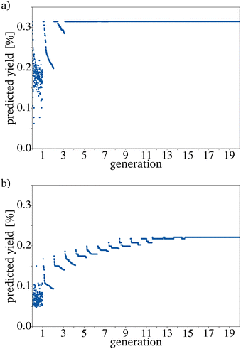
The catalysts proposed by the directed evolution in the last generation are very similar to each other. The resulting datasets can therefore be described as homogeneous. For a traditional evolutionary algorithm, this is expected if the algorithm converges in the set generation size G.39 Convergence is reached when the PY of the proposed catalysts stays similar. Convergence is reached faster if the size of the PG is increased, but even with small IGs e.g. 20, the algorithm proposes catalysts with an improved yield. This is also the case if the 100 catalysts with the highest yield in the database are used as input. If the picked catalysts have a low yield, it takes more mutation cycles to reach convergence. However, the difference between the average input yield and the average PY is larger compared to the evolution results based on the 100 catalysts with the highest yield (Fig. 6). This shows that the needed generation number depends strongly on the original PG. Depending on the dataset, a generation number that leads to convergence has to be found by trial and error. Since the mutation algorithm is quite fast, it is convenient to choose a generation number that is larger than the minimum number needed. How many generations are needed can be tested by using only the worst catalysts as the IG.Increasing E should lead to a faster convergence since more mutations are generated in each evolution cycle. Therefore, the probability of finding a catalyst with a higher yield in each mutation cycle is increased. Nevertheless, generating more mutations per evolution cycle leads to a longer runtime.
The expected effect of faster convergence with an increased E could be proven (Fig. 4a–c). Even though fewer generations were needed to reach convergence, the yield predicted for those catalysts started to decrease with a higher E. Since the PY and the number of generations needed to reach convergence strongly depend on the IG, the decision on which E to use can not be made based on the comparison of randomly picked original IGs (Fig. 4b)). The E giving the best results for the best possible original IG is 4. This means that you can work with only very few synthesized catalysts as starting point for a further data driven optimization via directed evolution. For the worst possible IG, E is 5. Since a lower E increases the number of necessary generations, for all further tests, an E of 4 has been used. Suppose each input catalyst results in many similar mutations close to the number of catalysts in the next IG. In that case, the generations get homogenous too fast and convergence is reached even though the PY is still low. Theoretically, for E = 4 and a generation size of 200 the next generation, picked from the third generation, can already be based entirely on one of the original IG catalysts. The number of generations until this point is reached increases with the generation size and decreases with a higher E (Fig. 5).
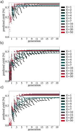 | ||
| Fig. 4 Evolution with a variation of E with a P of 100 for (a) the best, (b) randomly picked and (c) the worst catalysts. | ||
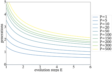 | ||
| Fig. 5 Generations that are needed until all catalysts picked for the next generation can theoretically be based on one catalyst of the original IG. | ||
If the homogenization of the next generation occurs too fast, the directed evolution tends to converge at a local optimum. To ensure this problem does not occur at least 25% of the mutations should be used as the new IG (E ≤ 4). If the generation size has to be small because the existing amount of data is small, the used E should be smaller than 4.
For most reactions in heterogeneous catalysis in general, the databases of tested catalysts are pretty small. Being able to reach a useful prediction based on an original PG consisting only of a few randomly picked catalysts is vital for smaller datasets. Fig. 6a–c show that the proposed algorithm works with only five catalysts in the IG. The limiting factor to using this algorithm is, therefore the dataset size necessary for training the RF. If the original IG is small, the needed generation number and also the proposed yield after reaching convergence strongly depends on each picked catalyst. This is made evident by the varying PY after convergence for five catalysts in the IG (Fig. 6a–c). A major problem with a small original IG is that the probability of reaching convergence at a low PY is increased because fewer mutations are evaluated per mutation cycle. Reaching premature convergence at a local optimum is caused when the picked catalysts for the next PG are very similar. For all further tests, a generation size of 200 has been picked. This is a bit more than 10% of the available catalysts and is still a small sample size but large enough to keep the probability of a coincidentally bad and homogenous original IG small.
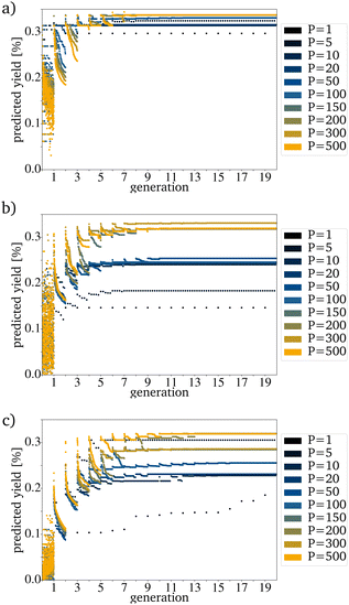 | ||
| Fig. 6 Evolution for a variation of P with an E of 1 for (a) the best, (b) randomly picked and (c) the worst catalysts. | ||
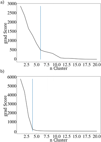
It is difficult to characterize the results of a directed evolution without testing the proposed catalysts in the lab. Since a homogeneous dataset is expected for the result of a traditional genetic algorithm as proposed here, it can be assumed that a successful evolution would lead to a homogeneous set of proposed catalysts. Clustering the catalysts is a tool to show how homogeneous the datasets of generated catalysts and the input dataset are. The proposed catalysts should be sortable into fewer clusters than the original dataset. Clustering the data is also useful for reducing the 68 dimensions of the catalyst to two dimensions that can be plotted.28 A so-called elbow curve can be used to find the minimal amount of clusters necessary to describe a dataset. The elbow curve (Fig. 7) for the last generation shows that four clusters are needed. The difference between the catalyst after the evolution is much lower compared to the original dataset, which required seven clusters.28
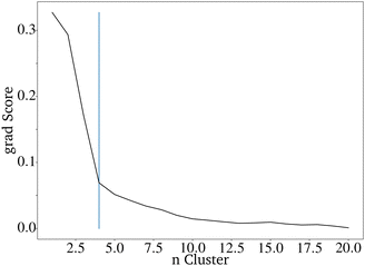 | ||
| Fig. 7 Elbow curve for the proposed catalysts of an directed evolution with E = 4, P = 200 and G = 20. | ||
Thermodynamic examination
DETCHEM EQUIL was used to evaluate if the yields proposed by the RF are thermodynamically possible.40 The highest C2 yield theoretically possible to reach is 37.8%. This is very close to the highest yield in the input data (37.0%). No yield proposed by the RF for the catalysts generated by the directed evolution is above 37.8%. This means that the proposed algorithm does not break the thermodynamical boundaries even though no thermodynamical laws are implemented directly. This effect is only based on the usage of machine learning for the evaluation step. All training data include the thermodynamical boundaries indirectly; therefore, the random forest follows them without implementing them directly. To ensure that no catalyst with a PY above the thermodynamical boundary is proposed, a check is implemented to verify this upper bound.If a yield above 0.378 is proposed by the RF function, an assertion error occurs. However, this has not happened once while testing.
Incorporating more parameters into the RF prediction
The OCM reaction can be carried out at various reaction temperatures and gas pressures. Even a mere inspection of the original dataset shows for example that the reaction temperature plays a key role in the OCM reaction. This leads to the assumption that including the reaction conditions as input parameters should improve the prediction. Also, the contact time can be varied over an extensive range.8 For example, the reaction temperature, the contact time, and the CH4 and O2 pressure could be included. It is relatively easy to incorporate those four parameters into the training of the RF. The preparation method of the catalyst and the reactor type in which the reaction is carried out can also affect the yield. There is no information about the reactor type in the used dataset. Additionally, the preparation method is not noted for all catalysts. The contact time, the reaction temperature and the gas pressures of CH4 and O2 were included to improve the RF. This increases the number of fitted parameters from 68 to 72 and the score on the training dataset to 0.91 and on the test dataset to 0.61. This function is also overfitted, but the 10% better score on the test dataset will lead to better predictions of the yield. Including more parameters makes the algorithm more complex and slower; therefore, being able to use only the catalyst composition as the input information would be an advantage. Before adding more dimensions, the disadvantages and advantages should always be weighed up against one another. Using four additional data points for the random forest training means that the evaluation of the catalysts generated by the directed evolution cannot be done based only on the composition of the catalysts. Therefore the reaction temperature is set to 1023 K, the contact time to 4.0 s, and the CH4 and O2 pressure to 0.1 and 0.05 bar. Those values were picked because they are the values for the catalyst with the best yield in the dataset. It should be possible to also predict those parameters with the help of machine learning and the same dataset. A similar implementation using the random forest algorithm for each parameter would be a straightforward approach but would need a lot more computing time. Interestingly the yields for the catalysts predicted by the RF are much lower after the same number of generations if the additional four factors are included (Fig. 8).Predicting the additional parameters instead of using the same four for all catalysts should improve this. The here used RF implementation is only capable to predict one target. Predicting additional targets would lead to the choice of another algorithm e.g. a Neural Network (NN). Unfortunately, this comes with drawbacks with respect to the data needed as NNs need typically more data than RF and more computational resources to fit the algorithm to the data. The reaction temperatures, contact times, and CH4 and O2 pressures vary a lot in the dataset. The higher accuracy of the RF should still lead to a better result of the directed evolution even if the PYs are low. In this case, a better result means that the PY is closer to the measured yield. The predicted reaction parameters hypothetically used in the evaluation step could also be a starting point for catalyst screening in the lab.
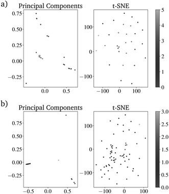
To compare the prediction with the RF with and without those additional parameters, the directed evolution was carried out 100 times with 100 different randomly picked IGs. For both evaluation methods, the number of metals included in the resulting dataset of 20.000 predicted catalysts was reduced drastically. Using the K-Means clustering algorithm shows that both datasets can be sorted into less than seven clusters, which are needed for the original dataset. The catalysts based on the directed evolution using the additional four properties can be sorted into only 4 clusters. For the catalysts based on the unimproved RF, at least 6 clusters are necessary (Fig. 9 and 10). This is higher than the clusters needed to describe only one last generation of the directed evolution. This shows that the improved RF evaluation leads to a more similar result than the unimproved RF evaluation if the directed evolution is carried out multiple times on different randomly picked datasets. Because the genetic algorithm works better with the improved RF function, the lower PY is not a disadvantage.
4 Comparison with real catalysts
All experiments have been carried out only in silico and have not been tested. The comparison with different publications of the last years shows that the proposed catalysts could be interesting to test. The directed evolution using the unimproved RF for evaluation proposes only 24 elements (Al, Ba, Ca, Ce, Cl, Ga, K, La, Li, Mg, Mn, Na, Nb, Nd, P, Pb, S, Si, Sn, Sr, Ti, W, Yb, Zn) as catalyst content and 22 (Ba, Br, Ca, Cl, Co, F, Fe, Gd, K, La, Li, Lu, Mg, Na, Ni, P, Pb, Rb, S, Sm, Sr) for the improved RF. The intersecting set of both results consists of 12 elements (Ba, Ca, Cl, K, La, Li, Mg, Na, P, Pb, S, Sr). The difference between both results is due to a little statistical effect since only 100 evolution cycles have been carried out for comparison. The difference in the evaluation step (68 or 72 dimensions of the RF function) has the main influence on the difference. The strong influence of the evaluation step implies that as many features as possible should be included to gain more reliable results. The proposed catalysts can be sorted into categories. The remaining 12% cannot be sorted into categories. For the unimproved RF, those categories are:(a) Mn (60%) with an additional alkali metal and sometimes another dopant (30%).
(b) Sr (50%), Ce (45%) and Yb (5%) (15%).
(c) Si (>50%) with Mn and Na and sometimes additional dopants (14%).
(d) A 3rd group metall (>90%) and small amounts of dopants (9%), Ti (60%) with other elements (6%).
(d) Ca (ca. 40%) and Cl (ca. 56%) with Pb and P as dopants (5%).
(e) La and an alkali metall (3%).
Most proposed pure metal catalysts would be challenging to prepare. However, oxides with similar metal contents can be found in literature. Catalyst with high Mn content as in category (a) are not part of recent and older research, but Nishimura et al.41 also suggest that Mn works as a promoter for the OCM reaction. Manganese oxides have long been the subject of research regarding OCM reaction catalysis.42 Many catalysts of this research fall into category (c) in which SiO2 is used as a support.43–45 For category (b) yields above 30% can be found in different reaction setups.46,47 Contrary to the work of Ferreira et al.48 Sr is proposed by the algorithm instead of Ca as a dopant for the CeO2 and MacHida et al.46 suggest that a Yb content of 0.1 leads to higher yields than a content of 0.05. Catalysts containing Ti as one of the main components as in (d) can also be found, as well as catalysts in group (g).49,50 The catalysts in category (f) are promising because it has been found that CaCl has a positive influence on ethene selectivity and Pb as a promoter enhances the catalytic activity.51
For the improved random forest, only four categories exist. The first category can be further subcategorized into three subcategories. The remaining 5% of the subcategories consists of a high Ca content and other dopants, which do not fit into the other three categories.
(a) Ca (>85%) with alkali metals, earth alkali metals and other dopants (53%)
(i) Ca (85%) with La and sometimes small amounts of Pb (27%)
(ii) Ca (>90%) and an alkali metal and other dopants (16%)
(iii) Ca (85%) and/or P and Pb (5%)
(b) Gd (>70%), Ba and a halogen (32%)
(c) Pure Lu (14%)
(d) A composite of similar amounts of Li, Fe, and Ba (2%)
Catalysts like (a) with a high Calcium content are mentioned repeatedly in the literature.51–53 The activity of those catalysts is based on the basicity of alkaline earth oxides and can be improved by introducing rare earth oxides e.g. Gadolinium.52 The suggested catalysts have not been subject of research in this exact composition. However, most categories are close enough to actual research that the results are a good starting point for synthesis. The exceptions are the catalysts with high Manganese content.
5 Conclusions
A real random mutation in synthesis is only possible for enzymatic catalysts. In silico mutation offers a possibility to apply this technique to heterogeneous catalysts. It has been shown that a simple approach for a genetic algorithm combined with an RF algorithm already leads to promising results for an in silico directed evolution. The simplicity of the approach makes it applicable to many datasets with only a small amount of changes. Those changes are primarily necessary for the step of data preprocessing. The usage of machine learning as a tool for catalyst evaluation is a promising route to replace the resource-intensive high throughput synthesis, bringing catalyst research to the 21st century by reducing waste and consumed energy. The proposed algorithm does not need a lot of computational resources and therefore is usable by most researchers.One of the major drawbacks of genetic algorithms is their tendency to premature convergence to local minima. The proposed algorithm also shows this problem. Therefore, a single-point crossover has been implemented to minimize this problem. Additionally, larger populations should be used if the used dataset allows it (Fig. 6).39 The single-point crossover is the most uncomplicated technique to implement and can be safely used since it produces acceptable solutions for almost all kinds of problems.54 Its major drawback is a slower performance and a higher risk for premature convergence. However, its simplicity and robustness still makes it favorable for this application.
Conflicts of interest
There are no conflicts to declare.Acknowledgements
This work was performed as part of the Cluster of Excellence Fuel Science Center (EXC 2186 ID: 390919832) funded by the Excellence Initiative by the German federal and state governments to promote science and research at German universities and NFDI4Cat as funded by the Deutsche Forschungsgemeinschaft (DFG, German Research Foundation) with the project number 441926934.Notes and references
- Y. Chu, W. Heyndrickx, G. Occhipinti, V. R. Jensen and B. K. Alsberg, J. Am. Chem. Soc., 2012, 134, 8885–8895 CrossRef CAS PubMed.
- O. Mamun, K. T. Winther, J. R. Boes and T. Bligaard, Sci. Data, 2019, 6, 1–9 CrossRef CAS PubMed.
- W. F. Maier, K. Stowe and S. Sieg, Angew. Chem., Int. Ed., 2007, 46, 6016–6067 CrossRef CAS PubMed.
- J. M. Caruthers, J. A. Lauterbach, K. T. Thomson, V. Venkatasubramanian, C. M. Snively, A. Bhan, S. Katare and G. Oskarsdottir, J. Catal., 2003, 216, 98–109 CrossRef CAS.
- S. Hahn, M. Dinarelli, C. Raymond, F. Lefèvre, P. Lehnen, R. De Mori, A. Moschitti, H. Ney and G. Riccardi, IEEE Trans. Audio, Speech Lang. Process., 2011, 19, 1569–1583 Search PubMed.
- T. Williams, K. McCullough and J. A. Lauterbach, Chem. Mater., 2020, 32, 157–165 CrossRef CAS.
- T. Toyao, Z. Maeno, S. Takakusagi, T. Kamachi, I. Takigawa and K.-I. Shimizu, ACS Catal., 2020, 10, 2260–2297 CrossRef CAS.
- U. Zavyalova, M. Holena, R. Schlögl and M. Baerns, ChemCatChem, 2011, 3, 1935–1947 CrossRef CAS.
- K. Takahashi, I. Miyazato, S. Nishimura and J. Ohyama, ChemCatChem, 2018, 10, 3223–3228 CrossRef CAS.
- G. E. Keller and M. M. Bhasin, J. Catal., 1982, 73, 9–19 CrossRef CAS.
- J. Garcia-Fayos, M. P. Lobera, M. Balaguer and J. M. Serra, Front. Mater., 2018, 5, 1–11 CrossRef.
- S. Da Ros, T. B. Fontoura, M. Schwaab, N. J. C. de Jesus and J. C. Pinto, Processes, 2021, 9, 2196 CrossRef CAS.
- T. N. Nguyen, T. T. P. Nhat, K. Takimoto, A. Thakur, S. Nishimura, J. Ohyama, I. Miyazato, L. Takahashi, J. Fujima, K. Takahashi and T. Taniike, ACS Catal., 2020, 10, 921–932 CrossRef CAS.
- B. L. Farrell and S. Linic, Catal.: Sci. Technol., 2016, 6, 4370–4376 RSC.
- S. Sourav, Y. Wang, D. Kiani, J. Baltrusaitis, R. R. Fushimi and I. E. Wachs, Angew. Chem., Int. Ed., 2021, 21502–21511 CrossRef CAS PubMed.
- R. Schmack, A. Friedrich, E. V. Kondratenko, J. Polte, A. Werwatz and R. Kraehnert, Nat. Commun., 2019, 10, 441 CrossRef CAS PubMed.
- G. V. Rossum, Proc. of the Nluug Najaarsconferentie, Dutch Unix Users Group, 1993, pp. 1-8.
- U. Gupta and D. G. Vlachos, J. Chem. Inf. Model., 2021, 61, 3431–3441 CrossRef CAS PubMed.
- E. D. Hermes, A. N. Janes and J. R. Schmidt, J. Chem. Phys., 2019, 151(1), 014112 CrossRef PubMed.
- Y. Lu, M. R. Farrow, P. Fayon, A. J. Logsdail, A. A. Sokol, C. R. A. Catlow, P. Sherwood and T. W. Keal, J. Chem. Theory Comput., 2019, 15, 1317–1328 CrossRef CAS PubMed.
- E. I. Ioannidis, T. Z. Gani and H. J. Kulik, J. Comput. Chem., 2016, 2106–2117 CrossRef CAS PubMed.
- S. O'Meara, S. Xu, D. Topping, G. Capes, D. Lowe, M. Alfarra and G. McFiggans, J. Open Source Softw., 2020, 5, 1918 CrossRef.
- B. Dahlgren, J. Open Source Softw., 2018, 3, 565 CrossRef.
- K. G. Prasanna, R. Sunil, K. Gupta and S. C. Lee, J. Comput. Chem., 2021, 42, 2116–2129 CrossRef PubMed.
- T. Gressling, Data Sci. Chem., 2020, 399–404 Search PubMed.
- M. F. Kasim, S. Lehtola and S. M. Vinko, J. Chem. Phys., 2022, 156, 084801 CrossRef CAS PubMed.
- E. J. Menke, J. Chem. Educ., 2020, 97, 3899–3903 CrossRef CAS.
- S. Palkovits, ChemCatChem, 2020, 12, 3995–4008 CrossRef CAS.
- F. H. Arnold, R. Swed. Acad. Sci., 2018, 50005, 1–10 Search PubMed.
- Y. Wang, P. Xue, M. Cao, T. Yu, S. T. Lane and H. Zhao, Chem. Rev., 2021, 121, 12384–12444 CrossRef CAS PubMed.
- F. H. Arnold, Angew. Chem., Int. Ed., 2018, 57, 4143–4148 CrossRef CAS PubMed.
- F. H. Arnold and A. A. Volkov, Curr. Opin. Chem. Biol., 1999, 3, 54–59 CrossRef CAS PubMed.
- V. Rodriguez-Galiano, M. Sanchez-Castillo, M. Chica-Olmo and M. Chica-Rivas, Ore Geol. Rev., 2015, 71, 804–818 CrossRef.
- T. Dietterich, ACM Comput. Surv., 1995, 27, 326–327 CrossRef.
- B. Ghojogh and M. Crowley, arXiv:1905.12787, 2019, 1–23 Search PubMed.
- F. H. Arnold, Acc. Chem. Res., 1998, 31, 125–131 CrossRef CAS.
- F. Clerc, M. Lengliz, D. Farrusseng, C. Mirodatos, S. R. Pereira and R. Rakotomalala, Rev. Sci. Instrum., 2005, 76(6), 062208 CrossRef.
- D. Wolf, O. V. Buyevskaya and M. Baerns, Appl. Catal., A, 2000, 200, 63–77 CrossRef CAS.
- S. F. Hwang and R. S. He, Adv. Eng. Inform., 2006, 20, 7–21 CrossRef.
- O. Deutschmann, S. Tischer, S. Kleditzsch, V. Janardhanan, C. Correa, D. Chatterjee, N. Mladenov, H. D. Minh, H. Karadeniz, M. Hettel, V. Menon, A. Banerjee, H. Goßler and E. Daymo, DETCHEM, 2020, https://www.detchem.com.
- S. Nishimura, J. Ohyama, X. Li, I. Miyazato, T. Taniike and K. Takahashi, Ind. Eng. Chem. Res., 2022, 61(24), 8462–8469 CrossRef CAS.
- L. M. Ioffe, P. Bosch, T. Viveros, H. Sanchez and Y. G. Borodko, Mater. Chem. Phys., 1997, 51, 269–275 CrossRef CAS.
- B. Beck, V. Fleischer, S. Arndt, M. G. Hevia, A. Urakawa, P. Hugo and R. Schomäcker, Catal. Today, 2014, 228, 212–218 CrossRef CAS.
- R. Koirala, R. Büchel, S. E. Pratsinis and A. Baiker, Appl. Catal., A, 2014, 484, 97–107 CrossRef CAS.
- U. Simon, O. Görke, A. Berthold, S. Arndt, R. Schomäcker and H. Schubert, Chem. Eng. J., 2011, 168, 1352–1359 CrossRef CAS.
- K. I. MacHida and M. Enyo, J. Chem. Soc., Chem. Commun., 1987, 21, 1639–1640 RSC.
- J. Langguth, R. Dittmeyer, H. Hofmann and G. Tomandl, Appl. Catal., A, 1997, 158, 287–305 CrossRef CAS.
- V. J. Ferreira, P. Tavares, J. L. Figueiredo and J. L. Faria, Ind. Eng. Chem. Res., 2012, 51, 10535–10541 CrossRef CAS.
- W. Pengwei, Z. Guofeng, W. Yu and L. Yong, Sci. Adv., 2017, 3, 1–9 Search PubMed.
- R. C. Schucker, K. J. Derrickson, A. K. Ali and N. J. Caton, Ind. Eng. Chem. Res., 2020, 59, 18434–18446 CrossRef CAS.
- J. H. Hong and K. J. Yoon, Appl. Catal., A, 2001, 205, 253–262 CrossRef CAS.
- R. V. Siriwardane, J. Catal., 1990, 123, 496–512 CrossRef CAS.
- A. M. Maitra, I. Campbell and R. J. Tyler, Appl. Catal., A, 1992, 85, 27–46 CrossRef CAS.
- O. Hasançebi and F. Erbatur, Comput. Struct., 2000, 78, 435–448 CrossRef.
Footnote |
| † The source for this manuscript is available at the following git repository https://git.rwth-aachen.de/palkovits/directedevolution2022_sourcecode. |
| This journal is © The Royal Society of Chemistry 2023 |

