
 Open Access Article
 This Open Access Article is licensed under a
 Creative Commons Attribution 3.0 Unported Licence
High-throughput computational workflow for ligand discovery in catalysis with the CSD†
Marc A. S.
Short
 a,
Clare A.
Tovee
c,
Charlotte E.
Willans
b and
Bao N.
Nguyen
*b
a,
Clare A.
Tovee
c,
Charlotte E.
Willans
b and
Bao N.
Nguyen
*b
aSchool of Chemical and Process Engineering, University of Leeds, Woodhouse Lane, Leeds LS2 9JT, UK
bSchool of Chemistry, University of Leeds, Woodhouse Lane, Leeds LS2 9JT, UK. E-mail: b.nguyen@leeds.ac.uk
cThe Cambridge Crystallographic Data Centre, 12 Union Road, Cambridge, CB2 1EZ, UK. E-mail: tovee@ccdc.cam.ac.uk
First published on 22nd March 2023
Abstract
A novel semi-automated, high-throughput computational workflow for ligand/catalyst discovery based on the Cambridge Structural Database is reported. Two potential transition states of the Ullmann–Goldberg reaction were identified and used as a template for a ligand search within the CSD, leading to >32![[thin space (1/6-em)]](https://www.rsc.org/images/entities/char_2009.gif) 000 potential ligands. The ΔG‡ for catalysts using these ligands were calculated using B97-3c//GFN2-xTB with high success rates and good correlation compared to DLPNO-CCSD(T)/def2-TZVPP. Furthermore, machine learning models were developed based on the generated data, leading to accurate predictions of ΔG‡, with 70.6–81.5% of predictions falling within ± 4 kcal mol−1 of the calculated ΔG‡, without the need for the costly calculation of the transition state. This accuracy of machine learning models was improved to 75.4–87.8% using descriptors derived from TPSS/def2-TZVP//GFN2-xTB calculations with a minimal increase in computational time. This new workflow offers significant advantages over currently used methods due to its faster speed and lower computational cost, coupled with excellent accuracy compared to higher-level methods.
000 potential ligands. The ΔG‡ for catalysts using these ligands were calculated using B97-3c//GFN2-xTB with high success rates and good correlation compared to DLPNO-CCSD(T)/def2-TZVPP. Furthermore, machine learning models were developed based on the generated data, leading to accurate predictions of ΔG‡, with 70.6–81.5% of predictions falling within ± 4 kcal mol−1 of the calculated ΔG‡, without the need for the costly calculation of the transition state. This accuracy of machine learning models was improved to 75.4–87.8% using descriptors derived from TPSS/def2-TZVP//GFN2-xTB calculations with a minimal increase in computational time. This new workflow offers significant advantages over currently used methods due to its faster speed and lower computational cost, coupled with excellent accuracy compared to higher-level methods.
1 Introduction
The development of organometallic catalysts, and suitable ligands, is a key challenge in the area of catalysis. While the process for traditional precious metals, such as Pd, Ru and Rh, is well established based on extensive mechanistic understanding and data-based approaches,1–7 ligand design for base metal catalysts is still a nascent area of research and needs to balance many more catalytic and catalyst decomposition pathways.8–10 Properties such as activity, selectivity and stability are the most common criteria when selecting a ligand, but solubility, toxicity and cost are also important properties to consider.11 Recent applications of data science to catalysis have highlighted the computer-guided search for optimal ligands and reaction conditions as a major technology which can significantly progress this field of research.12,13While high-throughput experimental approaches have proven effective at finding suitable ligands from libraries and optimising reaction conditions,14–17 these are limited by the available ligand libraries. In silico ligand exploration allows faster access to the entire chemical space and can lead to the discovery of unexpected ligands. In addition, new developments in high-throughput computational techniques,18–21 and cheminformatics tools can underpin additional filters such as ligand cost/complexity, toxicity and availability for a variety of applications in different chemical sectors.22–24 However, research in this field has been hampered by a lack of suitable tools for the automated exploration of ligand space, while taking into account synthetic feasibility of the ligands.13,25–27 In this paper, we report an alternative approach which leverages the extensive Cambridge Structural Database (CSD) and its tools to explore ligand space in a relevant catalytic reaction. This has the benefit of avoiding the synthetic feasibility challenge completely, while still maintaining a very wide chemical space coverage.
The approach was demonstrated with the copper(I)-catalysed Ullmann–Goldberg reaction, an important C–N cross-coupling reaction which has been highlighted by pharmaceutical companies as a desirable synthetic tool in the near future due to its mild conditions compared to the palladium-catalysed counterpart and sustainability credentials.28 Despite this level of interest, the Pd-catalysed Buchwald–Hartwig coupling reaction is still preferred due to its reliability and better-developed ligands. Several different reaction mechanisms have been proposed for this reaction, e.g. oxidative addition,29,30 single electron transfer (SET),31,32 atom transfer,31 sigma bond metathesis,33 and π-complexation of Cu(I) on ArX,34,35 which can depend on the substrates and ligands.36–39 The mechanisms are further complicated by reversible deactivation of the catalyst by reversible disproportionation of a Cu(I) intermediate into deactivated species,40–42 and involvement of the base in the reaction mechanism.43 Thus, little understanding of ligand design, which can improve reaction yields, scope, catalyst loading and catalyst stability, has been reported. This reaction serves as an excellent case study for our automated ligand discovery approach using the CSD and high-throughput calculation of activation energy barriers (Fig. 2). Two transition states, oxidative addition (TSOA) and sigma bond metathesis (TSSig), were chosen in this study. The other possible mechanisms, which require an accurate description of either open-shell complexes or weak interactions, were excluded due to the high computational cost required in a high-throughput context (Fig. 1).44–47
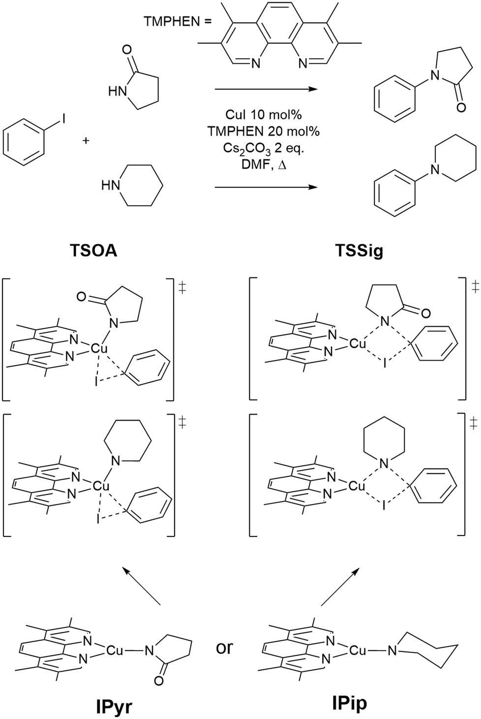 | ||
| Fig. 1 The Ullmann–Goldberg coupling reactions studied and proposed transition states for oxidative addition (TSOA) and sigma bond metathesis (TSSig). | ||
2 Methodology
2.1 Workflow for high-throughput catalyst design with the CSD
The workflow for the process of ligand identification from the CSD to building catalytic intermediates and transition states, to the calculation of activation energy barriers and machine learning (ML) descriptors are summarised in Fig. 2. The process is automated with Python. All automation code is included in the repository linked at the end of this manuscript.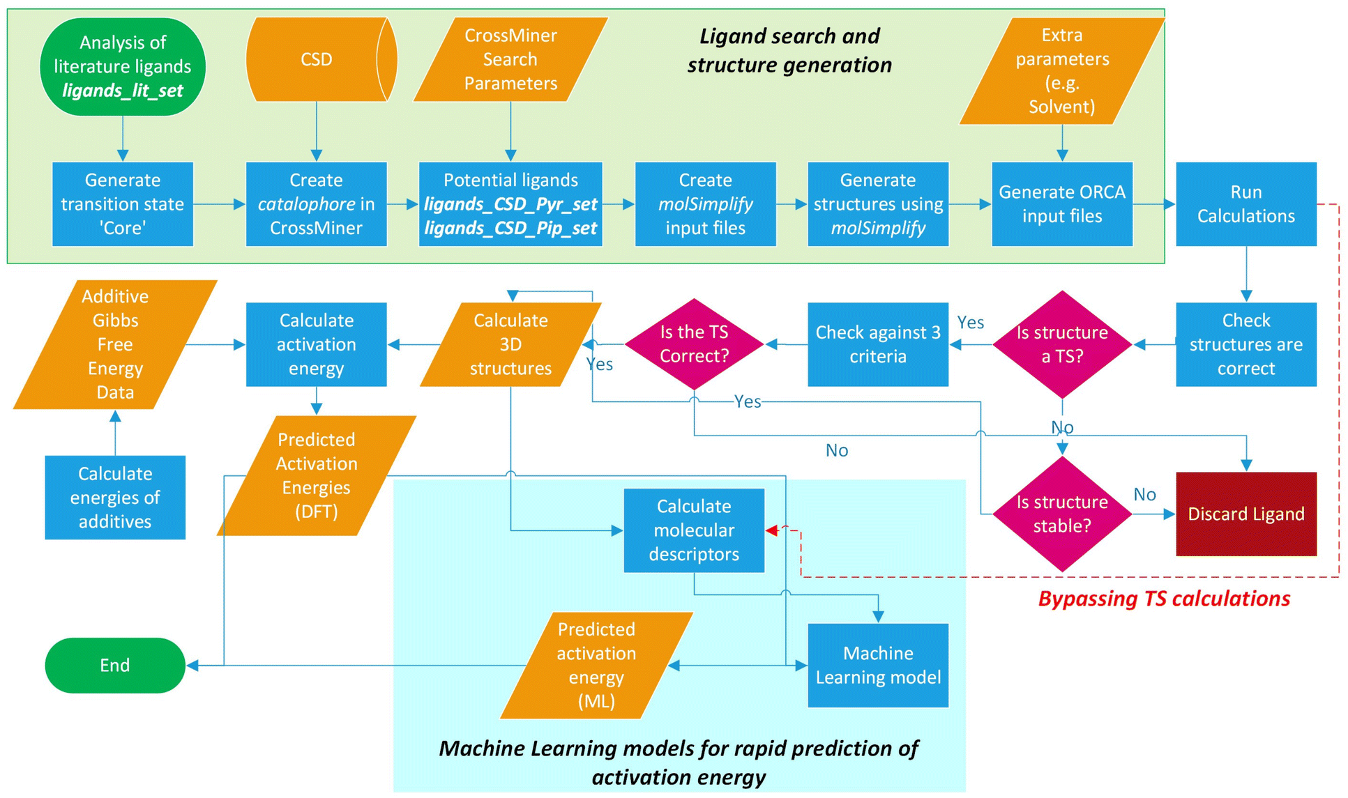 | ||
| Fig. 2 Workflow overview for identifying ligands in the CSD, high-throughput calculation of ΔG‡, and ML prediction of ΔG‡ for in silico screening of catalysts. | ||
2.2 Curation of literature ligands
Ligands were extracted from the Reaxys database for the C–N, C–O and C–S intermolecular Ullmann–Goldberg coupling, where the aryl halide is an aryl or heteroaryl chloride, bromide or iodide. For C–N coupling reactions, cyclic and acyclic amines and amides coupling partners were retrieved. Approximately 20000 reactions were identified. Ligands contained in precatalysts were extracted manually. Reactions with no identifiable ligand (e.g. copper nanoparticles) and no reported yield were removed resulting in a total of 10738, 2814, 750 entries for C–N, C–O and C–S coupling, respectively. From these entries, 345 unique ligands were identified. Structures of ligands were retrieved as a SMILES string using the Chemical Identifier Resolver (CIRpy).48 Where no structure was found, the structure was retrieved manually. Where structures contain multiple components, e.g. tetrabutylphosphonium acetate, the counterion or solvent was removed using the Openbabel Python toolkit. These ligands form the ligands_lit_set.
2.3 Ligands identification from the CSD
The CCDC CrossMiner tool was used to search the CSD for a catalophore, a 3D structural query made up of feature points describing the structural properties of the ligand and the desired transition state. These searches were performed on CSD_541 with the Mar20, May20, Aug20 and Feb21 updates. The following filters on structures were applied, leaving approximately 658000 structures: (a) are not polymeric, (b) have no disorder, (c) for which 3D coordinates have been determined and (d) have a maximum R-factor of 10%. A new set of features were created for catalysis to enable searching of the CSD for common coordinating functional groups, defined using SMARTS strings, in organometallic chemistry. The new database is named CatSD.
2.4 Building of complexes and transition states
A modified version of the molSimplify Python toolkit, which includes the additional ability for core-constrained force field optimisation, was employed to generate all structures.49 Ligands and substrates are supplied as either a SMILES string or an .xyz or .mol 3D structure file. Deprotonation of ligand functional groups upon coordination to the metal (i.e. OH and 1,3-dione) is achieved through functional group matching, using a set of deprotonation rules generated from the analysis of protonation states of similar Cu(I) complexes in the CSD (see ESI† Tables S2 and S3).Catalytic intermediates IPip and IPyr (Fig. 1) are generated through standard complex generation with piperidine and 2-pyrrolidinone as coupling partners, in a singlet spin state. The structures are optimised before and after ligand addition using the Universal Force Field (UFF).50 Transition state structures are generated via ligand replacement of a transition state template (TSOA or TSSig), generated with GFN2-xTB, using 3,4,7,8-tetramethyl-1,10-phenanthroline (TMPHEN) as the ligand, and iodobenzene as the aryl halide coupling partner. TMPHEN is then replaced using the ligand replacement feature included in molSimplify by defining the coordinating atoms of the new ligand(s). The structure is subsequently optimised with a custom after-core constrained method with UFF, where the transition state ‘core’ is locked and only the ligand(s) are optimised.
2.5 Molecular modelling
Benchmarking DFT calculations were performed in the gas phase using Gaussian09 Rev D.01.51 xTB, B97-3c and coupled cluster calculations were performed in ORCA 4.2.1 interfaced with xtb 6.3.3.19,52 ML DFT descriptor calculations use ORCA 5.0.1. Coupled cluster calculations were performed with the DLPNO-CCSD(T)/def2-TZVPP method.53 All DFT methods use the SMD solvent model with DMF as the solvent.54 GFN2-xTB methods use the generalised Born model with surface area contributions (GBSA) solvent model for DMF.55 Numerical Hessian were computed to determine the nature of the stationary points (zero and one for minima and transition states respectively) and to calculate the vibrational corrections at 298.15 K.For B97-3c//GFN2-xTB high-throughput calculations, the structures were first optimised and numerical frequencies were calculated with GFN2-xTB. Energy calculations were performed at the B97-3c level of theory using DMF as the solvent.
For transition state vetting, the eigenvector corresponding to the imaginary frequency should have motion along one of the transition state active bond stretching modes, with an overlap above the threshold S0 = 0.20 and 0.33 (eqn (2)) for TSOA and TSSig, respectively.
2.6 Energy and descriptor extraction
Gibbs free energies of simple reaction components, e.g. the base, counterions, and substrates, are calculated using standard protocols in DMF.Descriptors for ML were chosen to describe steric and electronic properties of the respective complexes and transition states. All electronic descriptors were extracted from the B97-3c energy files, except the imaginary frequency which is from the GFN2-xTB frequency calculation. Electronic descriptors: HOMO energy, LUMO energy, Lowdin charge, bonded valence, atomic population, bond order and orbital charges. Bond descriptors are for all transition state active bonds and Cu–L bonds. Electronic descriptors for individual atoms are for transition state active atoms and the ligand coordinating atoms, L1 and L2. Steric descriptors: bite angle, change in bite angle, cone angle, sterimol B1, B5, L, % buried volume at 3.5 Å, 5 Å and 7 Å, solvent accessible surface area, Cu–L bond lengths, bond angles and change in bond lengths between the transition state and CuLX starting structure, transition state active bond lengths and bond angles. Cu–L and transition state active steric descriptors were calculated directly from bond lengths and bond angles from the .xyz files. All other steric descriptors were calculated using the Morfeus Python package.56
2.7 Machine learning
Eight ML algorithms were employed; multiple linear regression (MLR), Gaussian process regression (GP), artificial neural networks (ANN), support vector machine (SVM), partial least squares (PLS), random forest (RF), extra trees (ET) and bagging (Bag). Default hyperparameters were tuned with the following exceptions: for GP only the Matern, radial basis function (RBF) and rational quadratic kernel were tuned; for ANN, n_odes (number of nodes in the hidden layers) was optimised with the number of hidden layers varied for SVM the RBF kernel was used with C, epsilon and gamma being optimised for PLS, n_components (number of components to retain after dimension reduction) was optimised and for RF, ET and bag, n_estimators (number of trees) and max_depth was optimised. These were optimised using the Optuna Python package, with performance metrics obtained using 10-fold cross-validation.57 ML was performed in Python 3 with the scikit-learn module. Prior to ML, all descriptors were scaled using a standard scaler. Models were set to optimise to a maximum for the coefficient of determination (R2). For the evaluation of prediction models for ΔG‡, datasets were split into training and test sets by binning the data in intervals of 1 kcal mol−1. A proportional amount of data was taken from each bin to form a training set (∼80% of the data) and a test set (∼20% of the data). Each model was trained on the same training set and tested on the same unseen test set.3 Results and discussion
3.1 Analysis of literature ligands and potential ligands in CSD
Analysis of literature Ullmann–Goldberg reactions contained within Reaxys resulted in 10728 C–N coupling reactions and 2814 C–O coupling reactions. From these, 345 literature ligands (281 bidentate and 64 monodentate) were extracted as the ligands_lit_set. The majority of bidentate ligands are N–N, O–O or N–O ligands, with only 7% containing a donating sulfur or phosphorus group. Importantly, 67% of the bidentate ligand contain a 2-atom bridge, 26% a 3-atom bridge, and 3% a 4-atom bridge (see ESI,† Tables S4 and S5). Given the dominance of bidentate ligands with a 2-atom bridge, they were selected as the preferred mode of coordination for the ligand search. A ligand with a 2-atom bridge and second-row donor atoms (N, O), i.e. TMPHEN, was selected for generating the template structure for each transition state which would be employed in the ligand search (Fig. 3).
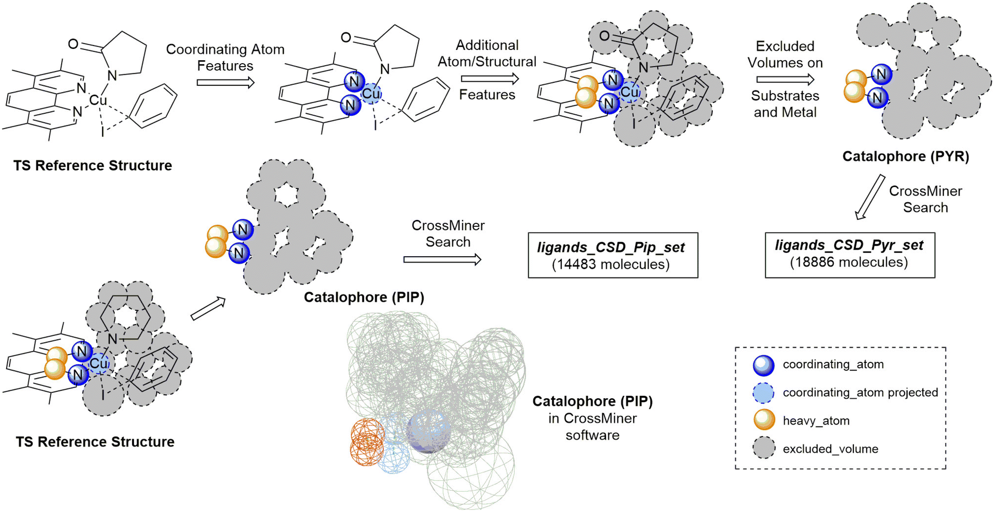 | ||
| Fig. 3 Workflow for generation of a catalophore from a transition state reference structure and identification ligands in the CSD to generate ligand sets ligands_CSD_Pip_set and ligands_CSD_Pyr_set. Hydrogens are excluded for clarity. | ||
For these transition states, piperidine and 2-pyrrolidinone were selected as coupling partners in order to minimise conformational flexibility in the organometallic intermediates and transition states (Fig. 1). In each case, a transition state was generated using GFN2-xTB using TMPHEN as the ligand, and iodobenzene as the aryl halide. The structure was optimised to a transition state and the imaginary frequency was checked for the correct vibrational mode (Fig. 3). These transition states were used as a reference structure for ligand identification in the CSD.
The TSOA structure with TMPHEN as the ligand was imported into CSD-CrossMiner and coordinating_atom features were placed on each TMPHEN nitrogen atom and projected onto the copper atom. A bridge of two heavy_atom features between the two coordinating nitrogens was placed on the two bridging carbon atoms. The tolerance for each atom was set at 0.75 Å after manual tuning. The features were constrained to be intramolecular. The substrate sites were defined by placing excluded volume features on each atom of the substrates with a tolerance equal to the van der Waals radii of the base atom. Thus, the created pocket represents the space occupied by both substrates in the transition state, with a soft tolerance allowing the vdW radii of atoms to overlap with the excluded cavity, to allow for variations in individual transition states with different ligands and substrates. Ligands which pre-arrange in this manner will more likely favour the required geometry of the transition state. Only organic structures were included in the search by setting is_organic to True. The catalophore was saved as a .cm file.
The catalophore searches were conducted using the CatSD structural database, a carefully curated subset of the CSD, with the CSD-PythonAPI. The searches were conducted with a maximum molecular weight of 500 Da, a maximum root-mean-square-deviation (RMSD) in geometry between catalophore and the hit of 1,58,59 with Br, Cl, I, Li, Na, K, Ca, Mg, Be and transition metals excluded. SMILES code matching was used to remove duplicate structures. 3D structures were cleaned by assigning all unknown bond types, adding all missing hydrogens and setting all formal charges. Structures were exported in .mol format. In order to generate organometallic complexes with the ligands, the indexes of the coordinating atoms in the 3D structure file are required to define the bonds between the ligand and the metal centre. These were automatically identified for each ligand by matching the coordinates of the coordinating_atom features to the atoms located at those coordinates in the hit structure. The atom indexes, name of the structure file and charge of the ligand are exported as a molSimplify .dict file. This .dict file is used by molSimplify to obtain the data required for structure generation for each ligand.
For piperidine and 2-pyrrolidinone coupling partners, 14483 (ligands_CSD_Pip_set) and 18886 (ligands_CSD_Pyr_set) unique structures were identified as potential ligands in the CSD, respectively.
3.2 Choice of computational methods
As very high-throughput computational studies of organometallic complexes and transition states is a relatively new area of research, there is no current consensus on the best methods for a given catalytic reaction. Thus, we decided to benchmark a wide range of semi-empirical and DFT methods (using the same basis set, def2-TZVP) for geometries of Cu(I) complexes and energies of transition states. All benchmarking complexes were taken from the CSD which contain the following: i) a mononuclear three-coordinate copper(I) centre, ii) a deprotonated N-ligand, iii) either one bidentate or two monodentate ligand(s). This led to a Cu_benchmark_set of 10 complexes with well-characterised structures (Fig. 4). The quality of the optimised structures is assessed on the basis of the reproduction of the coordination environment consisting of the metal–ligand bond lengths (d(Cu–L) in Å) and ligand–metal–ligand bond angles (∠(L–Cu–L) in °). The results are reported as the mean absolute error (MAE) against experimental values and are summarised in Table 1.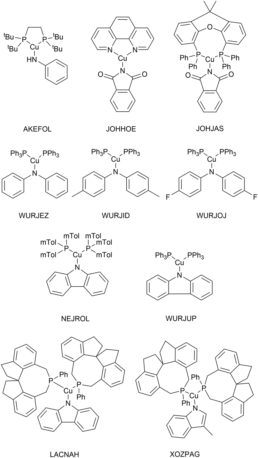 | ||
| Fig. 4 Structures of the 10 Cu(I) complexes in the Cu_benchmark_set. | ||
| Entry | Method/functional | MAE | Time (h) | |
|---|---|---|---|---|
| d(C–uL) (Å) | ∠(L–Cu–L) (°) | |||
| 1 | GFN0-xTB | 0.149 | 13.2 | 0.9 |
| 2 | GFN1-xTB | 0.073 | 4.6 | 2.0 |
| 3 | GFN2-xTB | 0.029 | 4.7 | 1.7 |
| 4 | HF-3c | 0.287 | 29.0 | 145 |
| 5 | PBEh-3c | 0.035 | 3.3 | 503 |
| 6 | B97-3c | 0.013 | 2.3 | 84 |
| 7 | B3LYP | 0.066 | 4.2 | 4931 |
| 8 | M06 | 0.034 | 3.4 | 7850 |
| 9 | M06-L | 0.020 | 4.1 | 7127 |
| 10 | TPSSh | 0.032 | 3.9 | 5435 |
| 11 | MPWLYP1M | 0.063 | 4.3 | 6508 |
| 12 | BP86 | 0.030 | 4.2 | 2143 |
| 13 | wB97xD | 0.030 | 4.3 | 9220 |
| 14 | B3LYP-D3(BJ) | 0.023 | 3.7 | 6179 |
| 15 | M06-D3(0) | 0.028 | 3.5 | 11140 |
| 16 | M06-L-D3(0) | 0.019 | 4.3 | 5271 |
| 17 | TPSSh-D3(BJ) | 0.016 | 3.3 | 6172 |
| 18 | TPSS-D3(BJ) | 0.017 | 3.7 | 3886 |
| 19 | PBE0-D3(BJ) | 0.018 | 3.6 | 5502 |
| 20 | BP86-D3(BJ) | 0.026 | 4.6 | 4036 |
Without D3 dispersion correction, all methods overestimated bond lengths by several picometers due to the inability of the methods to account for London dispersion interactions and increased steric interactions at the metal centres. The GGA/meta-GGA functionals, BP86 and M06-L, perform better than the hybrid functionals when predicting bond lengths, with BP86 being the most computationally efficient (entry 9 and 12, Table 1). The inclusion of D3 dispersion correction led to significantly improved performance in all DFT methods. TPSSh, a meta-GGA hybrid including 10% HF exchange, showed the best predictions for both bond lengths and bond angles while keeping the computational cost relatively low. Importantly, GFN2-xTB calculations using xtb 6.3.0 with verytight optimisation criteria showed excellent structural agreement with the crystal structures with minimal computational cost (entry 3, Table 1). The composite method B97-3c gave even better results (MAE of 0.013 Å and 2.3°), requiring only 84 hours of single-core CPU time, compared to 6172 hours for TPSSh-D3(BJ) and 4036 hours for BP86-D3(BJ). In fact, B97-3c outperformed the best DFT functional TPSSh-D3(BJ), even with a full triple-ζ basis set. Thus, the GFN2-xTB and B97-3c methods are the most suitable computational methods for very high-throughput computational studies of the Ullmann–Goldberg reaction (Fig. 5).
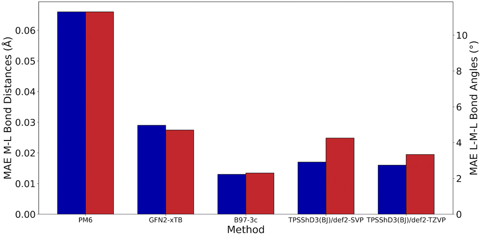 | ||
| Fig. 5 Geometrical benchmarking results for the best-performing methods in each class (semi-empirical, extended tight binding, 3c and DFT), mean absolute error in metal–ligand bond length (blue) and ligand–metal–ligand bond angle (red), for the Cu_benchmark_set. | ||
Lastly, the accuracy of the high-throughput calculation of ΔG‡ for the Ullmann–Goldberg reaction was assessed. Grimme and co-workers have demonstrated that the B97-3c//GFN2-xTB combination can be as accurate as traditional DFT methods in optimising and calculating energy-related properties of stable organometallic compounds.21,60 However, its performance in calculating transition states is unknown. Thus, we benchmarked the accuracy of B97-3c//GFN2-xTB calculated ΔG‡ values (B97-3c single point energy with GFN2-xTB vibrational correction) against those obtained by the ‘gold standard’ method for the calculation of structure energies, CCSD(T), for 100 randomly selected literature ligands. Both energy calculations used the same GFN2-xTB optimised structures. Coupled cluster energies were calculated at the DLPNO-CCSD(T)/def2-TZVPP level of theory and compared to the B97-3c energy. The results are summarised in Fig. 6.
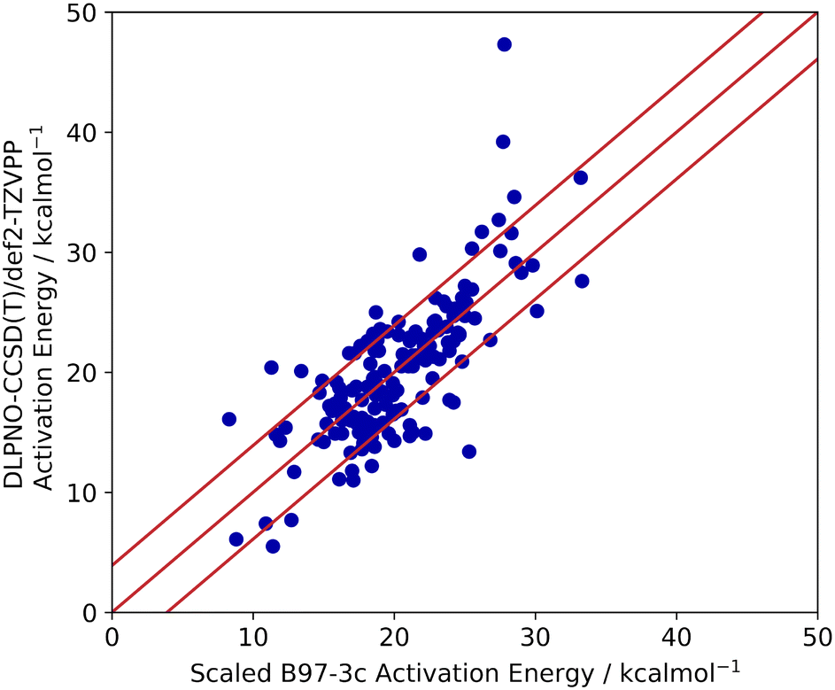 | ||
| Fig. 6 Scaled B97-3c activation energies of 68 TSOA and 83 TSSig transition states from ligands_lit_set, compared to their DLPNO-CCSD(T)/def2-TZVPP calculated activation energies. The red lines represent 3.9 kcal mol−1 (the MAE in the calculations). | ||
The activation energies barriers calculated by B97-3c were found to correlate reasonably well with those obtained with DLPNO-CCSD(T)/def2-TZVPP method (R2 = 0.5774 for a linear relationship y = 0.8938x + 8.3679). Therefore, the B97-3c derived values were scaled (see ESI,† section 2.2), achieving a mean average error (MAE) of 3.9 kcal mol−1 (Fig. 6). The majority of calculated ΔG‡ (89%) fell with 15× RMSE of the benchmarked values. Thus, the B97-3c method represents a good balance between computational time and accuracy for the calculation of activation energies of Ullmann–Goldberg reactions. Structures containing oximes and O–Cu–O 5-membered ring motifs correlate poorly between the two methods. However, only 8 ligands containing oximes have been reported for the Ullmann–Goldberg reaction (ligands_lit_set), and this was not deemed a significant problem for ligand exploration.
Based on the benchmarking results all optimisations and frequency calculations were performed using GFN2-xTB. Energy calculations were carried out using the B97-3c composite method.
3.3 High-throughput calculation of ΔG‡
Once the potential ligands were identified, all corresponding structures of catalytic intermediates and TSOA and TSSig transition states for each of the ligands were generated using a modified version of molSimplify.49 There are two key challenges in automating this process: (i) determining the coordination sites in ligands with more than 2 feasible sites (ligands_lit_set only); and (ii) determining whether deprotonation of any coordination site is required prior to coordinating to Cu(I). The first challenge was addressed via a combinatory approach, generating all possible bidentate combinations between the ligand and Cu(I) cation. The second challenge was addressed via analysis of Cu(I) complexes of similar ligands. For this, the CSD was searched for Cu(I) complexes with each functional group (e.g. alcohol, amine) both with and without the presence of a proton (e.g. OH–Cu and O–Cu). The number of search results for each indicated whether the functional group should be protonated or deprotonated during complex generation (see ESI,† Tables S2 and S3). Generally, functional groups with a pKa < 25 (DMSO) were deprotonated upon coordination.Conversion of ligands into complexes using SMARTS/SMILES strings and rdkit package can suffer from conformational variation from those in the CSD. Thus, ligands are taken as .xyz or .mol 3D structure files derived from their structures in the CSD. For ligands_lit_set, SMILES strings were used due to the lack of suitable 3D structures in the CSD, and monodentate ligands were excluded for simplicity.
In order to automate the generation of transition states TSOA and TSSig, a different strategy was employed. The transition states generated with TMPHEN above were employed as templates and TMPHEN was substituted with the ligand of interest. These structures were then pre-optimised with a custom after-core constrained method using the universal force field (UFF), where the transition state ‘core’ is locked and only the ligand is optimised to ensure the transition state mode is preserved.
The structures generated by molSimplify were pre-optimised with GFN2-xTB with the TightOpt optimisation criteria with the transition state active atoms frozen. The resulting structure was considered close to the transition state and was then optimised using eigenvector following to the transition state. To ensure reliability in cases with a shallow PES the exact Hessian is calculated every five optimisation steps. The presence of a transition state is verified by the presence of a single imaginary frequency. Single point energies are calculated with B97-3c using the TightSCF criteria and SlowConv to improve the reliability of SCF convergence. It is worth noting that many potential energy surfaces for TSOA and TSSig are relatively flat, requiring frequency Hessian calculations which are more costly computationally.
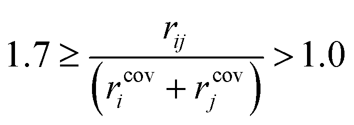
Preliminary examination of automated results showed that the process is prone to generating wrong transition states, e.g. a methyl rotation, dissociation of reactants, no identified transition state and hydrogen transfer between the ligand and the amine/amide. In order to validate the computed transition states, the vetting criteria presented by Jacobsen et al. were used.61 This procedure is not based on an IRC calculation and, therefore, reduces the required computational time. The transition state structure must meet the following three criteria: i) exactly one imaginary frequency of the Hessian (a cutoff value of −40 cm−1 is used to remove structures with frequencies that could be considered as numerical noise); ii) the transition state active bonds (bonds being broken or formed) must be of an intermediate length (eqn (1)),
 | (1) |
| |vstretchi·vts| ≥ S0 | (2) |
To assess the accuracy of the workflow in generating and optimising the transition states, 198 ligands from ligands_CSD_Pip_set were used as test cases. Both oxidative addition (TSOA) and sigma metathesis (TSSig) transition states with piperidine as the N-partner were generated and optimised. Manual inspection of the structures and visualisation of the imaginary frequency of a subset of ligands gave an optimal value of S0 = 0.20 and 0.33 for TSOA and TSSig respectively, for the Ullmann–Goldberg reaction. For intermediates CuLI and IPip, 98% of all structures containing bidentate ligands were successfully generated (Table 2). For optimisation, 80% of CuLI and 56% of IPip structures were correctly optimised in an automated manner. Compared to these, the optimisation of transition states was very successful, giving a success rate of 63% for TSOA and 88% for TSSig. The most common reason for optimisation failure is low imaginary vibrational frequencies (>−20 cm−1). This is likely due to poor starting structures generated from SMILES strings. To mitigate this on the CSD datasets, all structures (ligands and nucleophiles) were supplied as either X-ray or optimised 3D structures and the TightOpt criteria was used to aid the removal of small imaginary frequencies.
When this workflow was applied to the entire ligands_CSD_Pip_set and ligands_CSD_Pyr_set, the optimisation success rates for stable intermediates were significantly higher than those for ligands_lit_set, thanks to the initial 3D ligand structures supplied from the CSD. On the other hand, the success rates for transition states are significantly lower than those of ligands_lit_set. The success rate of finding and optimising TSOA (33%) was particularly low using ligands_CSD_Pip_set (Table 2). This result reflects that many potential ligands are not suitable for the Ullmann–Goldberg coupling reaction, as suggested by the experimental literature. TSSig is less sterically demanding than TSOA and consequently resulted in better success rates with both ligand sets. Similarly, as 2-pyrrolidinone is less sterically demanding than piperidine, the success rate in optimising TSOA is significantly higher with ligands_CSD_Pyr_set comparing to that with ligands_CSD_Pip_set.
The real-world runtime on a high-performance computing system using 4 cores and 4GB of RAM per job for ligands_CSD_Pip_set is ∼6 weeks for 14483 ligands. The comparative time for ligands_CSD_Pyr_set is ∼4 weeks for 18886 ligands after fine-tuning.
3.4 Factors influencing ΔG‡ of the Ullmann–Goldberg reaction
Previous computational studies on Pd-catalysed reactions have shown the dependence of ΔG‡ on the electronic properties of the ligand and its bite angle.62,63 Understanding similar relationships in Cu(I)-catalysed coupling reactions is an important milestone in ligand design for these catalysts. Thus, an analysis of the properties of the calculated transition states and their relationship to the calculated ΔG‡ was performed. These properties were selected to represent the steric and electronic properties of the catalytic centre in the TS, which should influence its stability and the calculated ΔG‡. A full table of properties/descriptors is available in the ESI† (section 5.4.4). Particular attention was given to the steric descriptors, given the shorter Cu–C/N/O bonds compared to those of palladium. Surprisingly, no clear relationship with individual descriptors was observed with any of the four sets of calculated transition states(Pyr_set_TSOA, Pyr_set_TSSig, Pip_set_TSOA, and Pyr_set_TSSig). All properties of both the TS and the starting intermediate have little to no impact on ΔG‡ (see ESI† Table S11). This highlights the unique nature of Cu(I) d10 catalytic centre, which is less sensitive to the ligand field and electronic properties of the ligand. The activation energy distributions for ligands_CSD_PIP_set are similar across both transition states with an average ΔG‡ of ∼18 kcal mol−1 (Fig. 7a). Closer examination showed the values for each ligand are generally close, with a small number of ligands giving very low or very high ΔG‡ for TSOA with piperidine as the N-partner (Fig. 8). With 2-pyrrolidinone as the N-partner, there is a clear difference in ΔG‡ between the TSOA (∼18 kcal mol−1) and TSSig (∼38 kcal mol−1) transition states. This suggests that for an amide nucleophile, the oxidative addition pathway is energetically more favourable than the sigma metathesis pathway. This difference in energy is likely due to the strain introduced to the amide bond, the N-atom changing from a trigonal planar to tetrahedral geometry, in the TSSig transition state. On the whole, TSOA is often either more favourable or as likely as TSSig in this type of Ullmann–Goldberg coupling reaction.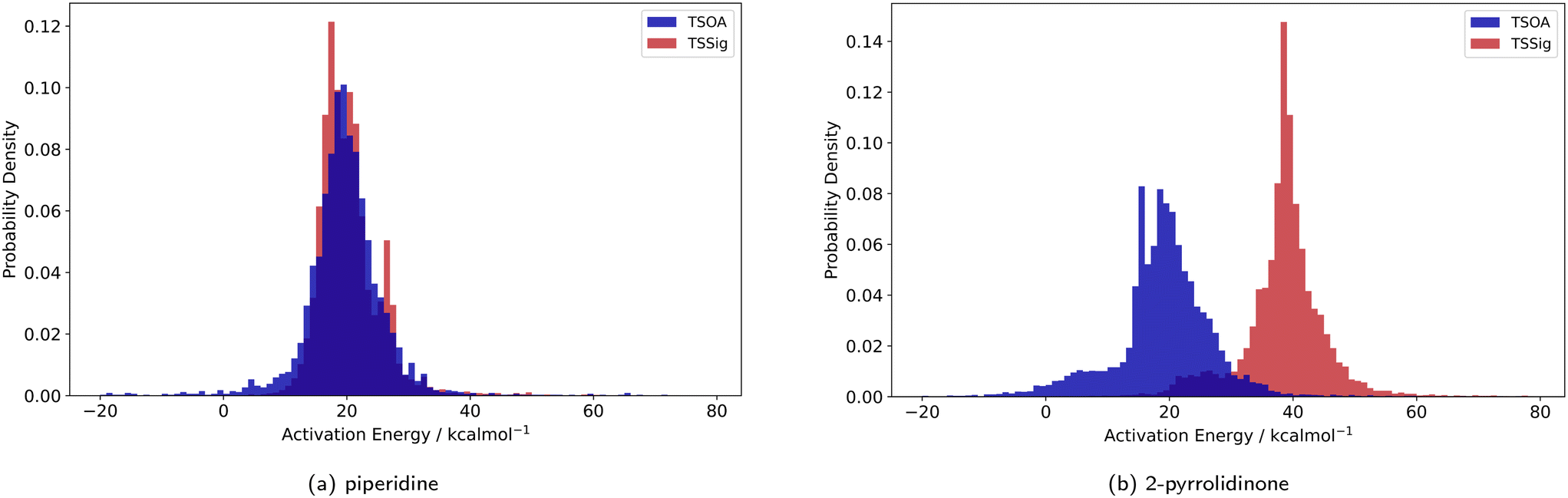 | ||
| Fig. 7 Probability density for the activation energies of the TSOA (blue) and TSSig (red) transition states for piperidine (left) and 2-pyrrolidinone (right). | ||
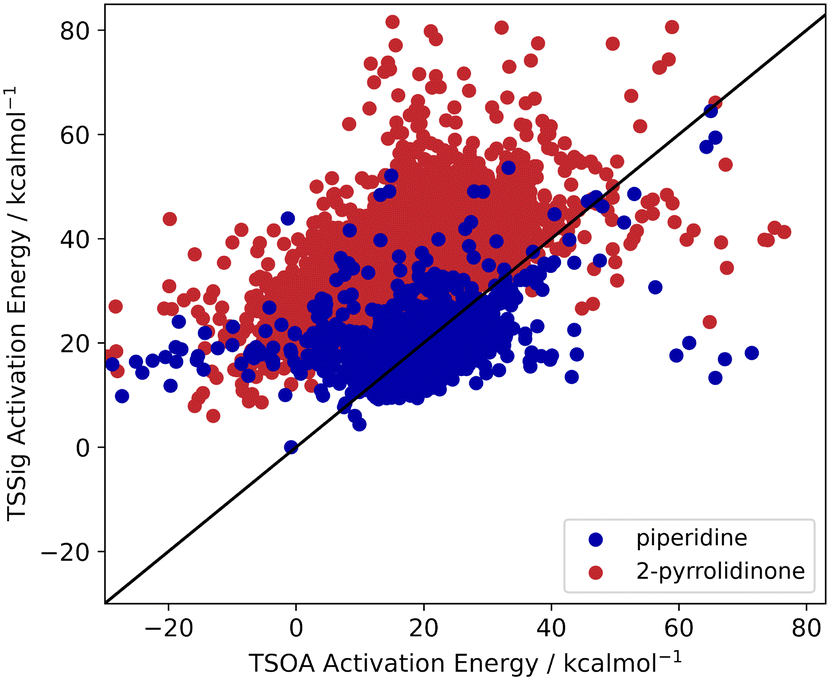 | ||
| Fig. 8 TSOA activation energy against TSSig activation energy for piperidine (blue) and 2-pyrrolidinone (red). | ||
3.5 Predicting ΔG‡ with machine learning
![[double bond, length as m-dash]](https://www.rsc.org/images/entities/char_e001.gif) O bonds, and associated charges and molecular orbitals). In order to improve interpretability, the descriptors were trimmed by removing all but one highly correlated descriptor based on Pearson's coefficient (Table 3).
O bonds, and associated charges and molecular orbitals). In order to improve interpretability, the descriptors were trimmed by removing all but one highly correlated descriptor based on Pearson's coefficient (Table 3).
| Dataset | Original | Highly correlated removed | Low importance removed |
|---|---|---|---|
| TS dependent | |||
| PIP_set_TSOA | 78 | 75 | 20 |
| PYR_set_TSOA | 128 | 111 | 24 |
| PIP_set_TSSig | 91 | 90 | 36 |
| PYR_set_TSSig | 130 | 121 | 41 |
| TS independent | |||
|---|---|---|---|
| PIP_set_TSOA_NoTS | 67 | 60 | 10 |
| PYR_set_TSOA_NoTS | 67 | 62 | 14 |
| PIP_set_TSSig_NoTS | 67 | 61 | 27 |
| PYR_set_TSSig_NoTS | 67 | 62 | 17 |
Common practice in ML relies on R2 and RMSE, which do not consider the level of noise in training data, to evaluate models. Consequently, a new metric was created to evaluate the models: % of ΔG‡ prediction within ± 4 kcal mol−1 (%ΔG‡ ± 4). This reflects the maximum accuracy of the model based on the error present in the DFT calculated activation energies. Calculated datasets were trimmed via binning to remove bias from the uneven distribution of activation energies. Entries with a Cu–L bond order of 0 were discarded as they were bonding in a monodentate manner.
| Dataset | Best algorithm | R 2 | RMSE | %ΔG‡ ± 4 |
|---|---|---|---|---|
| Full descriptors | ||||
| PIP_set_TSOA | ET | 0.49 | 7.90 | 75.5 |
| PYR_set_TSOA | ET | 0.65 | 6.32 | 66.1 |
| PIP_set_TSSig | ET | 0.39 | 5.93 | 77.9 |
| PYR_set_TSSig | ET | 0.63 | 5.52 | 68.5 |
| Trimmed descriptors | ||||
|---|---|---|---|---|
| PIP_set_TSOA | ET | 0.66 | 4.81 | 79.6 |
| PYR_set_TSOA | ET | 0.71 | 4.86 | 71.3 |
| PIP_set_TSSig | ET | 0.48 | 4.33 | 81.5 |
| PYR_set_TSSig | ET | 0.66 | 4.95 | 70.6 |
The importance of each descriptor was evaluated using permutation importance over 50 runs.64 Those which showed a permutation importance of mean − 2 × std ≤ 0 (mean = average decrease in R2 over 50 runs, std = standard deviation of the decrease in R2 over 50 runs; this metric means that more than 95% of the permutation importance values from 50 runs are above 0) were removed. This led to a very significant reduction in the number of descriptors in each dataset (Table 3), improving the interpretability of the prediction models. Importantly, the removal of the redundant descriptors led to improvement in all metrics by a significant margin (Table 4).
|
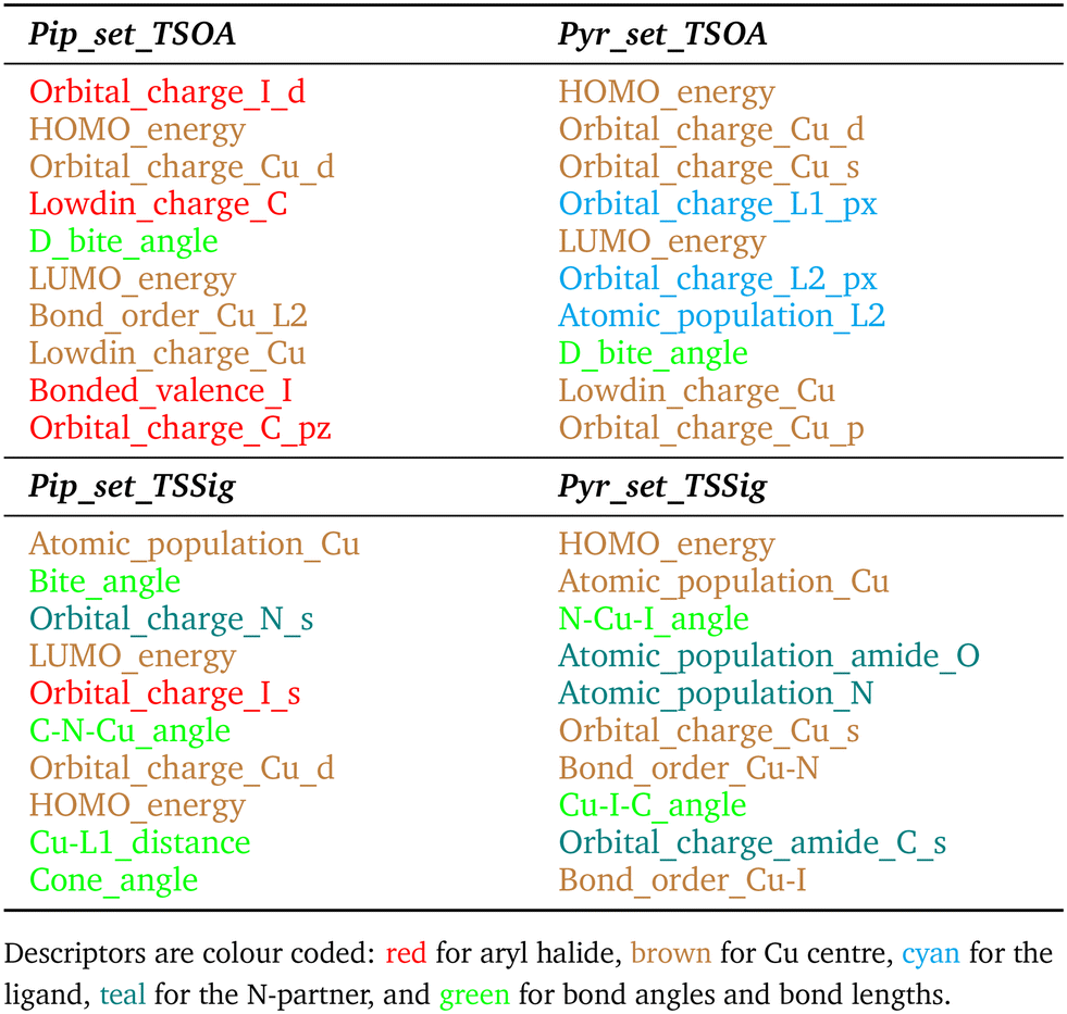
For TSSig, ΔG‡ showed high dependence on the atomic population on the Cu centre, Cu–N and Cu–I bond orders and TS mode bond angles, HOMO/LUMO energies and orbital charges of the Cu s, d, N s and I d orbitals. The sigma metathesis pathway showed strong dependence on steric descriptors (distances and angles). The amide C–O bond length and C–N bond order are important properties for coupling with 2-pyrrolidinone. This implies that the ability of the ligand to modulate the electron density of the copper centre to bond to and weaken the amide bond in the nucleophile is important. For piperidine, no such trend was observed, indicating a lesser degree of influence from the amine partner beyond a direct sigma donation to the Cu centre.
| Structure | Single-core computational time (h) | |||
|---|---|---|---|---|
| Optimisation | Energy + frequency | Total | % of time | |
| Ligands_CSD_PIP_set | ||||
| CuLI | 66 | 6244 | 6310 | 3.5 |
| IPip | 169 | 9897 | 10067 |
5.6 |
| TSOA | 102971 |
15373 |
118336 |
65.6 |
| TSSig | 30829 |
14957 |
45787 |
25.4 |
| Ligands_CSD_PYR_set | ||||
|---|---|---|---|---|
| CuLI | 1173 | 8596 | 9789 | 6.0 |
| IPyr | 1693 | 11618 |
13312 |
8.2 |
| TSOA | 69212 |
17949 |
87162 |
53.6 |
| TSSig | 33253 |
19212 |
52466 |
32.2 |
For this purpose, only descriptors based on IPyr and IPip were selected and subjected to the same descriptor trimming process (Table 3). Descriptors for individual atoms were extracted for Cu, N and ligand coordinating atoms (L1 and L2). For ligands_CSD_PYR_set, descriptors were also extracted for the amide C and O atoms. This resulted in four datasets, PIP_set_TSOA_NoTS, PIP_set_TSSig_NoTS, PYR_set_TSOA_NoTS and PYR set_TSSig_NoTS containing 67 descriptors and 1683, 3708, 3990 and 5798 ligands respectively (Fig. 9).
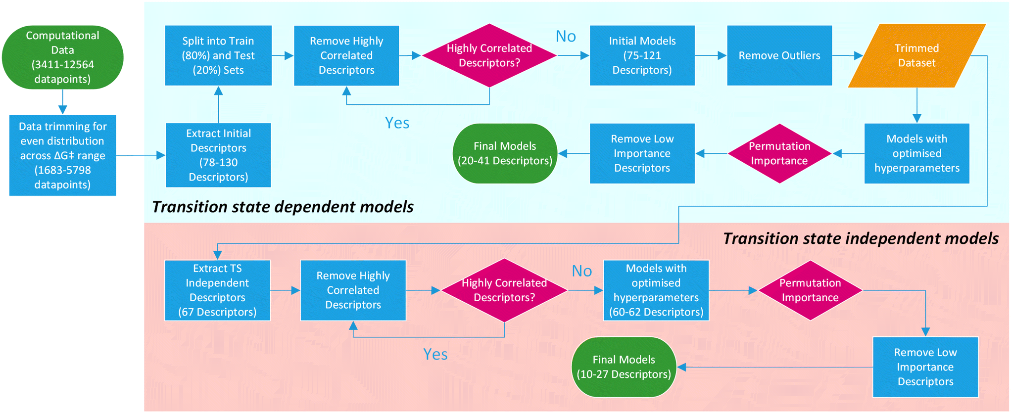 | ||
| Fig. 9 Overview of the machine learning model generation process, from computational data to final models. | ||
The results for the transition state independent models, using the same algorithms, are summarised in Table 7. Predictably, these new models show reduced accuracy compared to those with descriptors from the transition states, except for PYR_set_TSOA_NoTS which shows a slight improvement in R2 (0.67 to 0.69) and RMSE (5.16 to 4.97). Nevertheless, the significant reduction of computational time (5.7–10 times) for new predictions with only a small decrease in accuracy was promising.
| Dataset | Best algorithm | R 2 | RMSE | %ΔG‡ ± 4 |
|---|---|---|---|---|
| Full descriptors | ||||
| PIP_set_TSOA_NoTS | SVM | 0.32 | 6.56 | 79.6 |
| PYR_set_TSOA_NoTS | SVM | 0.67 | 5.16 | 68.1 |
| PIP_set_TSSig_NoTS | SVM | 0.57 | 3.74 | 83.7 |
| PYR_set_TSSig_NoTS | ET | 0.66 | 4.83 | 75.8 |
| Trimmed descriptors | ||||
|---|---|---|---|---|
| PIP_set_TSOA_NoTS | ET | 0.29 | 6.95 | 76.3 |
| PYR_set_TSOA_NoTS | ET | 0.69 | 4.97 | 66.4 |
| PIP_set_TSSig_NoTS | SVM | 0.56 | 3.78 | 82.8 |
| PYR_set_TSSig_NoTS | ET | 0.64 | 4.98 | 75.8 |
| PBE0 electronic descriptors | ||||
|---|---|---|---|---|
| PIP_TSOA_PBE0 | SVM | 0.40 | 6.11 | 82.3 |
| PYR_TSOA_PBE0 | SVM | 0.71 | 4.59 | 72.6 |
| PIP_TSSig_PBE0 | SVM | 0.69 | 3.78 | 84.6 |
| PYR_TSSig_PBE0 | ET | 0.68 | 4.66 | 78.0 |
| TPSS electronic descriptors | ||||
|---|---|---|---|---|
| PIP_TSOA_TPSS | ET | 0.34 | 6.03 | 80.5 |
| PYR_TSOA_TPSS | SVM | 0.69 | 4.27 | 75.4 |
| PIP_TSSig_TPSS | ET | 0.62 | 3.46 | 87.8 |
| PYR_TSSig_TPSS | ET | 0.70 | 4.09 | 80.4 |
In order to improve the prediction models for ΔG‡ without calculating the transition states, some of the freed-up computational time was dedicated to the calculation of more accurate electronic descriptors using a higher-level method. The electronic descriptors were recalculated using three DFT methods: TPSS, TPSSh and PBE0. These were selected for their previous successful calculation of first-row transition metals complexes (TPSS) and increasing amount of Hartree–Fock exchange for more accurate bonding description (TPSSh and PBE0).65,66 The triple-ζ basis set def2-TZVP was used with all methods. The single-core CPU time for each energy method for 50 IPip/IPyr structures is 14, 34, 94 and 86 hours for B97-3c, TPSS, TPSSh and PBE0, respectively. The correlation of electronic descriptors and activation energy with those from DLNPO-CCSD(T)/def2-TZVPP were examined (see ESI,† Table S28), and PBE0 and TPSS were selected for prediction model building based on either accuracy or speed. In each case, the new ΔG‡ values from PBE0 or TPSS replaced the values from B97-3c in these models.
Surprisingly, the TPSS-based models outperformed those based on PBE0 with better RMSE metrics across all four datasets, requiring only a third of the CPU time compared to that of PBE0. On average, the computational time per new prediction of ΔG‡ was reduced from ∼10 h, for transition state based B97-3c//GFN2-xTB models, to ∼1 h using TPSS-def2-TZVP//GFN2-xTB descriptors based on IPyr or IPip. The predictions for the PIP_TSSig_TPSS dataset are well within the error of the calculated activation energies (3.9 kcal mol−1). These are very significant improvements to the B97-3c//GFN2-xTB models both with and without the inclusion of the transition state descriptors. This new method using ML algorithms to predict ΔG‡ provides an excellent balance between accuracy and speed for high-throughput ligand/catalyst development.
Lastly, the trend in descriptor importance is consistent between the transition state dependent and transition state independent models. The TSOA ΔG‡ is dependent on the ability of the ligand to modulate the electron density at the copper centre via the s/d orbitals. The lack of amine nitrogen descriptors within the top 5 most important descriptors, after which change in R2 drops significantly, implies that the interaction between the copper and nucleophile is of low importance, which can be justified by the lack of N participation in the oxidative addition transition state. The TSSig ΔG‡ is dependent on the ability of the ligand to create the correct orientation and modulate the electron density on the nucleophile nitrogen. In the case of an amide nucleophile, this is achieved through the weakening of the amide bond.
4 Conclusions
We have presented a novel semi-automated, high-throughput computational workflow for ligand/catalyst development based on the prediction of ΔG‡ in copper(I)-catalysed C–N coupling reactions and the CSD. This workflow (i) automatically generates organometallic intermediates and transition states, (ii) performs computational calculations for the determination of structural and electronic properties, and (iii) analyses and predicts the activation energy for each ligand. Importantly, ML models were developed based on the high-throughput computational output to accurately predict the activation energy barriers while bypassing the costly calculation of the transition states. These models performed very well against the “gold-standard” coupled-cluster method, with typically 75–88% of predictions < ± 4 kcal mol−1 at a much lower computational cost. Models were analysed to identify potentially important ligand features for the design of new catalysts.This workflow offers significant advantages over currently used methods due to its faster speed and good to excellent accuracy compared to higher-level methods. We expect this workflow to have wide applicability in catalyst design, ranging from pharmaceutical process development to novel catalyst design across multiple chemical areas. Further development toward fully automated processes is in progress and will benefit the wider chemistry community.
Data availability
All code used in the presented work is freely available via Zenodo at https://doi.org/10.5281/zenodo.7390425 with all the datasets presented in this manuscript.Author contributions
M. A. S. S. carried out the data analysis and all the computational and machine learning work. B. N. N., C. E. W. and C. A. T. provided scientific insights and guided the direction of the project. The manuscript was written by M. A. S. S. and B. N. N.Conflicts of interest
There are no conflicts to declare.Acknowledgements
This research was carried out at the EPSRC Centre for Doctoral Training in Complex Particulate Products and Processes (EP/S022473/1) as part of a collaborative project with the Cambridge Crystallographic Data Centre (CCDC), who we gratefully acknowledge.Notes and references
- J. Lu, S. Donnecke, I. Paci and D. C. Leitch, Chem. Sci., 2022, 13, 3477–3488 RSC.
- T. Gensch, G. dos Passos Gomes, P. Friederich, E. Peters, T. Gaudin, R. Pollice, K. Jorner, A. Nigam, M. Lindner-D’Addario, M. S. Sigman and A. Aspuru-Guzik, J. Am. Chem. Soc., 2022, 144, 1205–1217 CrossRef CAS PubMed.
- N. Fey, A. Koumi, A. V. Malkov, J. D. Moseley, B. N. Nguyen, S. N. G. Tyler and C. E. Willans, Dalton Trans., 2020, 49, 8169–8178 RSC.
- D. J. Durand and N. Fey, Chem. Rev., 2019, 119, 6561–6594 CrossRef CAS PubMed.
- J. Jover, N. Fey, J. N. Harvey, G. C. Lloyd-Jones, A. G. Orpen, G. J. J. Owen-Smith, P. Murray, D. R. J. Hose, R. Osborne and M. Purdie, Organometallics, 2012, 31, 5302–5306 CrossRef CAS PubMed.
- N. Fey, J. N. Harvey, G. C. Lloyd-Jones, P. Murray, A. G. Orpen, R. Osborne and M. Purdie, Organometallics, 2008, 27, 1372–1383 CrossRef CAS.
- N. Fey, A. C. Tsipis, S. E. Harris, J. N. Harvey, A. G. Orpen and R. A. Mansson, Chem. – Eur. J., 2006, 12, 291–302 CrossRef CAS PubMed.
- B. Cheng, H. Yi, C. He, C. Liu and A. Lei, Organometallics, 2015, 34, 206–211 CrossRef CAS.
- C. Poree and F. Schoenebeck, Acc. Chem. Res., 2017, 50, 605–608 CrossRef CAS PubMed.
- G. J. Sherborne, S. Adomeit, R. Menzel, J. Rabeah, A. Brückner, M. R. Fielding, C. E. Willans and B. N. Nguyen, Chem. Sci., 2017, 8, 7203–7210 RSC.
- J.-P. Lange, Nat. Catal., 2021, 4, 186–192 CrossRef CAS.
- K. Wu and A. G. Doyle, Nat. Chem., 2017, 9, 779–784 CrossRef CAS PubMed.
- H. J. Kulik and M. S. Sigman, Acc. Chem. Res., 2021, 54, 2335–2336 CrossRef CAS PubMed.
- Y. Amar, A. M. Schweidtmann, P. Deutsch, L. Cao and A. Lapkin, Chem. Sci., 2019, 10, 6697–6706 RSC.
- D. T. Ahneman, J. G. Estrada, S. Lin, S. D. Dreher and A. G. Doyle, Science, 2018, 360, 186–190 CrossRef CAS PubMed.
- A. F. Zahrt, J. J. Henle, B. T. Rose, Y. Wang, W. T. Darrow and S. E. Denmark, Science, 2019, 363, 1–11 CrossRef PubMed.
- H. Tian and S. Rangarajan, J. Chem. Theory Comput., 2019, 15, 5588–5600 CrossRef CAS PubMed.
- S. Dohm, M. Bursch, A. Hansen and S. Grimme, J. Chem. Theory Comput., 2020, 16, 2002–2012 CrossRef CAS PubMed.
- C. Bannwarth, E. Caldeweyher, S. Ehlert, A. Hansen, P. Pracht, J. Seibert, S. Spicher and S. Grimme, WIREs Comput. Mol. Sci., 2021, 11, e1493 CAS.
- C. Bannwarth, S. Ehlert and S. Grimme, J. Chem. Theory Comput., 2019, 15, 1652–1671 CrossRef CAS PubMed.
- M. Bursch, H. Neugebauer and S. Grimme, Angew. Chem., Int. Ed., 2019, 58, 11078–11087 CrossRef CAS PubMed.
- M. H. S. Segler, M. Preuss and M. P. Waller, Nature, 2018, 555, 604–610 CrossRef CAS PubMed.
- C. W. Coley, W. H. Green and K. F. Jensen, Acc. Chem. Res., 2018, 51, 1281–1289 CrossRef CAS PubMed.
- K. L. Dobo, N. Greene, C. Fred, S. Glowienke, J. S. Harvey, C. Hasselgren, R. Jolly, M. O. Kenyon, J. B. Munzner, W. Muster, R. Neft, M. Vijayaraj Reddy, A. T. White and S. Weiner, Regul. Toxicol. Pharmacol., 2012, 62, 449–455 CrossRef CAS PubMed.
- M. Foscato and V. R. Jensen, ACS Catal., 2020, 10, 2354–2377 CrossRef CAS.
- D. V. S. Green, S. Pickett, C. Luscombe, S. Senger, D. Marcus, J. Meslamani, D. Brett, A. Powell and J. Masson, J. Comput.-Aided Mol. Des., 2020, 34, 747–765 CrossRef CAS PubMed.
- Y. Chu, W. Heyndrickx, G. Occhipinti, V. R. Jensen and B. K. Alsberg, J. Am. Chem. Soc., 2012, 134, 8885–8895 CrossRef CAS PubMed.
- S. M. Mennen, C. Alhambra, C. L. Allen, M. Barberis, S. Berritt, T. A. Brandt, A. D. Campbell, J. Castañón, A. H. Cherney, M. Christensen, D. B. Damon, J. Eugenio de Diego, S. García-Cerrada, P. García-Losada, R. Haro, J. Janey, D. C. Leitch, L. Li, F. Liu, P. C. Lobben, D. W. C. MacMillan, J. Magano, E. McInturff, S. Monfette, R. J. Post, D. Schultz, B. J. Sitter, J. M. Stevens, I. I. Strambeanu, J. Twilton, K. Wang and M. A. Zajac, Org. Process Res. Dev., 2019, 23, 1213–1242 CrossRef CAS.
- G. Lefèvre, G. Franc, A. Tlili, C. Adamo, M. Taillefer, I. Ciofini and A. Jutand, Organometallics, 2012, 31, 7694–7707 CrossRef.
- J. W. Tye, Z. Weng, A. M. Johns, C. D. Incarvito and J. F. Hartwig, J. Am. Chem. Soc., 2008, 130, 9971–9983 CrossRef CAS PubMed.
- G. O. Jones, P. Liu, K. N. Houk and S. L. Buchwald, J. Am. Chem. Soc., 2010, 132, 6205–6213 CrossRef CAS PubMed.
- H. L. Aalten, G. van Koten, D. M. Grove, T. Kuilman, O. G. Piekstra, L. A. Hulshof and R. A. Sheldon, Tetrahedron, 1989, 45, 5565–5578 CrossRef CAS.
- V. V. Litvak and U. S. M. Shein, Zh. Org. Khim., 1974, 10, 2360 CAS.
- J. Lindley, Tetrahedron, 1984, 40, 1433–1456 CrossRef CAS.
- H. Weingarten, J. Org. Chem., 1964, 29, 3624–3626 CrossRef CAS.
- C. Sambiagio, S. P. Marsden, A. J. Blacker and P. C. McGowan, Chem. Soc. Rev., 2014, 43, 3525–3550 RSC.
- E. Sperotto, G. P. M. van Klink, G. van Koten and J. G. de Vries, Dalton Trans., 2010, 39, 10338–10351 RSC.
- H.-Z. Yu, Y.-Y. Jiang, Y. Fu and L. Liu, J. Am. Chem. Soc., 2010, 132, 18078–18091 CrossRef CAS PubMed.
- P.-F. Larsson, A. Correa, M. Carril, P.-O. Norrby and C. Bolm, Angew. Chem., Int. Ed., 2009, 48, 5691–5693 CrossRef CAS PubMed.
- R. Giri, A. Brusoe, K. Troshin, J. Y. Wang, M. Font and J. F. Hartwig, J. Am. Chem. Soc., 2018, 140, 793–806 CrossRef CAS PubMed.
- G. J. Sherborne, S. Adomeit, R. Menzel, J. Rabeah, A. Brückner, M. R. Fielding, C. E. Willans and B. N. Nguyen, Chem. Sci., 2017, 8, 7203–7210 RSC.
- J. Tye, Z. Weng, R. Giri and J. Hartwig, Angew. Chem., Int. Ed., 2010, 49, 2185–2189 CrossRef CAS PubMed.
- K. K. Gurjar and R. K. Sharma, ChemCatChem, 2017, 9, 862–869 CrossRef CAS.
- A. Nandy and H. Kulik, ACS Catal., 2020, 10, 15033–15047 CrossRef CAS.
- F. Liu, C. Duan and H. J. Kulik, J. Phys. Chem. Lett., 2020, 11, 8067–8076 CrossRef CAS PubMed.
- C. Duan, J. P. Janet, F. Liu, A. Nandy and H. J. Kulik, J. Chem. Theory Comput., 2019, 15, 2331–2345 CrossRef CAS PubMed.
- A. Nandy, J. Zhu, J. P. Janet, C. Duan, R. B. Getman and H. J. Kulik, ACS Catal., 2019, 9, 8243–8255 CrossRef CAS.
- N. C. Institute, Chemical Identifier Resolver, 2020, https://cactus.nci.nih.gov/chemical/structure Search PubMed.
- E. Ioannidis, T. Gani and H. Kulik, J. Comput. Chem., 2016, 37, 2106–2117 CrossRef CAS PubMed.
- A. Rappé, C. Casewit, K. Colwell, W. Goddard and W. M. Skiff, J. Am. Chem. Soc., 1992, 114, 10024–10035 CrossRef.
- M. J. Frisch, G. W. Trucks, H. B. Schlegel, G. E. Scuseria, M. A. Robb, J. R. Cheeseman, G. Scalmani, V. Barone, G. A. Petersson, H. Nakatsuji, X. Li, M. Caricato, A. V. Marenich, J. Bloino, B. G. Janesko, R. Gomperts, B. Mennucci, H. P. Hratchian, J. V. Ortiz, A. F. Izmaylov, J. L. Sonnenberg, D. Williams-Young, F. Ding, F. Lipparini, F. Egidi, J. Goings, B. Peng, A. Petrone, T. Henderson, D. Ranasinghe, V. G. Zakrzewski, J. Gao, N. Rega, G. Zheng, W. Liang, M. Hada, M. Ehara, K. Toyota, R. Fukuda, J. Hasegawa, M. Ishida, T. Nakajima, Y. Honda, O. Kitao, H. Nakai, T. Vreven, K. Throssell, J. A. Montgomery, Jr., J. E. Peralta, F. Ogliaro, M. J. Bearpark, J. J. Heyd, E. N. Brothers, K. N. Kudin, V. N. Staroverov, T. A. Keith, R. Kobayashi, J. Normand, K. Raghavachari, A. P. Rendell, J. C. Burant, S. S. Iyengar, J. Tomasi, M. Cossi, J. M. Millam, M. Klene, C. Adamo, R. Cammi, J. W. Ochterski, R. L. Martin, K. Morokuma, O. Farkas, J. B. Foresman and D. J. Fox, Gaussian 09 Revision D.01, Gaussian Inc., Wallingford CT, 2009 Search PubMed.
- F. Neese, WIREs Comput. Mol. Sci., 2018, 8, e1327 Search PubMed.
- C. Riplinger, B. Sandhoefer, A. Hansen and F. Neese, J. Chem. Phys., 2013, 139, 134101 CrossRef PubMed.
- A. V. Marenich, C. J. Cramer and D. G. Truhlar, J. Phys. Chem. B, 2009, 113, 6378–6396 CrossRef CAS PubMed.
- A. Onufriev, D. Bashford and D. A. Case, Proteins: Struct., Funct., Bioinf., 2004, 55, 383–394 CrossRef CAS PubMed.
- GitHub - kjelljorner/morfeus: A Python package for calculating molecular features — github.com, https://github.com/kjelljorner/morfeus#readme, [Accessed 31-May- 2022].
- T. Akiba, S. Sano, T. Yanase, T. Ohta and M. Koyama, Proceedings of the 25rd ACM SIGKDD International Conference on Knowledge Discovery and Data Mining, 2019 Search PubMed.
- W. Kabsch, Acta Crystallogr., Sect. A: Cryst. Phys., Diffr., Theor. Gen. Crystallogr., 1976, 32, 922–923 CrossRef.
- O. Korb, B. Kuhn, J. Hert, N. Taylor, J. Cole, C. Groom and M. Stahl, J. Med. Chem., 2016, 59, 4257–4266 CrossRef CAS PubMed.
- J. G. Brandenburg, C. Bannwarth, A. Hansen and S. Grimme, J. Chem. Phys., 2018, 148, 064104 CrossRef PubMed.
- L. D. Jacobson, A. D. Bochevarov, M. A. Watson, T. F. Hughes, D. Rinaldo, S. Ehrlich, T. B. Steinbrecher, S. Vaitheeswaran, D. M. Philipp, M. D. Halls and R. A. Friesner, J. Chem. Theory Comput., 2017, 13, 5780–5797 CrossRef CAS PubMed.
- P. Vermeeren, X. Sun and F. M. Bickelhaupt, Sci. Rep., 2018, 8, 10729 CrossRef PubMed.
- W.-J. van Zeist, R. Visser and F. Bickelhaupt, Chem. – Eur. J., 2009, 15, 6112–6115 CrossRef CAS PubMed.
- L. Breiman, Mach. Learn., 2001, 45, 5–32 CrossRef.
- M. Bühl and H. Kabrede, J. Chem. Theory Comput., 2006, 2, 1282–1290 CrossRef PubMed.
- M. P. Waller, H. Braun, N. Hojdis and M. Bühl, J. Chem. Theory Comput., 2007, 3, 2234–2242 CrossRef CAS PubMed.
Footnote |
| † Electronic supplementary information (ESI) available. See DOI: https://doi.org/10.1039/d3cy00083d |
| This journal is © The Royal Society of Chemistry 2023 |