 Open Access Article
Unsupervised classification of voltammetric data beyond principal component analysis†
Christopher
Weaver
 a,
Adrian C.
Fortuin
 ab,
Anton
Vladyka
 a and
Tim
Albrecht
 *a
*a
aSchool of Chemistry, University of Birmingham, Edgbaston Campus, Birmingham B15 2TT, UK. E-mail: t.albrecht@bham.ac.uk
bFaculty of Mechanical Engineering, Helmut Schmidt University, 22043 Hamburg, Germany
First published on 17th August 2022
Abstract
In this study, we evaluate different apoproaches to unsupervised classification of cyclic voltammetric data, including Principal Component Analysis (PCA), t-distributed Stochastic Neighbour Embedding (t-SNE), Uniform Manifold Approximation and Projection (UMAP) as well as neural networks. To this end, we exploit a form of transfer learning, based on feature extraction in an image recognition network, VGG-16, in combination with PCA, t-SNE or UMAP. Overall, we find that t-SNE performs best when applied directly to numerical data (noise-free case) or to features (in the presence of noise), followed by UMAP and then PCA.
Voltammetric data contain a wealth of mechanistic, kinetic, and analytical information about the system under study and are routinely used in a wide range of applications, including for the basic characterisation of redox-active materials,1 surface characterisation2 and the study of electrocatalytic processes.3 In some cases, the amount of available data is small and their analysis can readily be performed ‘by hand’. Typically, this information is extracted based on theoretical models, for example in relation to the dependence of peak currents on analyte concentration or scan rate, to mass transport and the effect of electrode geometry or the overall shape of the voltammetric signal.4,5 Deviations from model behaviour can significantly enhance the complexity of the task, but may be addressed using numerical modelling or calibration.6
In other applications, however, data are recorded in an (semi-) automated way and are then much more abundant. Examples include high-throughput screening,7 autonomous sensing and quality control,8 and electrochemical surface imaging.9 This calls for automated analysis methodologies, which is relatively straightforward, if the system behaviour is well-understood, robust and well-defined. In such cases, specific observables, such as the current at given potential or the peak current, may be used to extract the quantity of interest.
However, the analysis task becomes significantly more challenging, if this is not the case. For example, the data may reflect a mixture of different electrochemical processes, be recorded under varying geometrical conditions or be affected by device failure or contamination.10,11 In such cases, unsupervised dimensionality reduction techniques such as PCA have been employed, which to some extent consider the overall appearance of the data.12–15 Beyond PCA, there are however other, potentially superior dimensionality reduction techniques, such as non-linear, stochastic methods, which aim to reproduce neighbourhood relations in high-dimensional data space in a lower dimensional representation. Those have not found widespread application in electrochemistry yet and we will therefore explore two examples, namely t-SNE16,17 and UMAP,18,19 and benchmark those against an implementation of linear PCA. Supervised methodologies, which do require labelled training data, have been introduced to the field recently and show promise for some applications.20–23 However, they will not be in focus here. In addition to the three dimensionality reduction techniques mentioned above, we will also consider three different data input formats and evaluate their effect on the classification performance. These are raw numerical data (i.e. (scaled) current-potential value pairs), b/w images of the CVs as well as the feature extractor output of an image recognition network, VGG-16, as illustrated in Fig. 1.24,25 The latter is based on the idea that such networks are able to identify salient features in physico-chemical data, despite initially being trained on unrelated image data of everyday objects. We recently demonstrated this approach for single-molecule charge transport data using another image recognition network, AlexNet,24,26 and were able to identify previously undetected sub-populations in the data. Interestingly, while this has elements of transfer learning or Artificial General Intelligence, the fact that the feature extractor does not require re-training also demonstrates that such Deep Learning architectures can be employed successfully in the absence of large amounts of, or indeed any, domain-specific data.
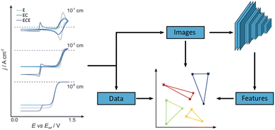 | ||
| Fig. 1 Schematic of the unsupervised classification process (right) alongside examples of simulated CVs (left). CVs were simulated for ‘E’ (grey), ‘EC’ (light blue), and ‘ECE’ (dark blue) reaction mechanisms at varying electrode radii. In general, CVs are pre-processed in three formats: images; features; and data. The data and image sets are created by taking the datapoint or converting graphs into images, respectively. The Features dataset is created by utilising a pretrained VGG-16 CNN feature extractor. See ESI,† and main text for more details on the simulation and analysis pipeline. | ||
In order to establish an unequivocal “ground truth”, we use simulated data (Digisim® v3.0), in some cases with added noise (vide infra). A total of 18 CVs was generated for three different, classic electrochemical reaction mechanisms, namely electron transfer (E), electron transfer coupled with a homogeneous chemical reaction (EC) and a sequence of electron transfer/homogeneous chemical reaction/electron transfer (ECE), for electrode radii ranging from 10−1 to 10−6 cm, Fig. 1. This choice is to some extent arbitrary and mainly served to generate well-defined, distinct cyclovoltammetric responses. However, the specific thermodynamic and kinetic model parameters were taken from a well-known and well-characterised example, namely the electrochemical oxidation of aniline to polyaniline, see Sections S1 and S2 in the ESI† for further details.27,28
The raw numerical data values were scaled between −1 and 1 (comparable to the image data), in order to emphasize shape, rather than the magnitude of the current, and to facilitate a comparison with the analysis of other input formats used in this study. In practical applications, the electrode radius is normally given, but changes in appearance could conceivably have other origins.
After dimensionality reduction, each CV was represented in a two-dimensional projection, with each E/EC/ECE triplet spanning a triangle of perimeter P, where larger P scores correspond to better separation between the three mechanisms (each component scaled from 0 to 1, so 0 ≤ P ≤ 2 +  ; over all 18 CVs). In addition, to quantify the separation of triplets, we used the mean silhouette value of each triplet, as defined in eqn (1):
 | (1) |
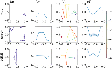
Considering dimensionality reduction applied directly to the raw (value pair) data first, the different metrics are summarised in Fig. 2. Column (a) shows the value triplet for r = 1 × 10⁻¹ cm, for PCA (top), UMAP (centre) and t-SNE (bottom), see Fig. 1. For this particular radius, PCA produces a point triplet that is roughly equally separated, even if the perimeter score is relatively small. It is larger for other electrode radii, column (b), and reaches a maximum for r = 1 × 10⁻⁴ cm. Under these conditions, the E and EC mechanisms produce very similar CVs, which is reflected in a rather large, but irregular triangle in the reduced dimensional representation, column (c). Based on the S score and an optimised set of hyperparameters, column (d), separation by electrode radius works best for the small and large radii, less so for the intermediate range. This is in part a manifestation of the interdependence of the perimeter and silhouette score metrics, as large perimeter values are more likely to result in overlap between adjacent point triplets and hence reduced silhouette values. However, we have used this approach to facilitate the comparison across the entire dataset as well as between the different dimensionality reduction techniques. Notably, when optimised for maximum perimeter score, UMAP and t-SNE produce larger P scores, compared to PCA, suggesting that those two techniques provide better separation between the three mechanisms. However, to account for the stochastic nature of both UMAP and t-SNE, where the outcome can show some variation from run to run, we show averages of P and S, as well as associated 95% confidence intervals for UMAP and t-SNE (20 repeats each), as shown in Fig. 2(b) and (d). In terms of P score and across all electrode radii, UMAP broadly follows the trend observed in the PCA results, while t-SNE appears to show a more consistent performance throughout.
The UMAP and t-SNE results shown in columns (c) and (d) are optimised for maximum S score. Normalised over the entire dataset, it becomes apparent that some ability to differentiate between mechanisms is lost (small P scores for large r, for example), but that those triplets are then well-separated from the others (relatively high S score). Conversely, at intermediate radii, separation by mechanism is still satisfactory (relatively large triangles), but separation between electrode radii is decreased (triplet overlap). In any case, hyperparameter optimisation clearly has an effect on the result of the classification.
We now compare the performance of PCA, UMAP and t-SNE when applied to the CVs, presented as image data. The results are summarised in Fig. 3. As before, we focus on a specific electrode radius in column (a), namely r = 1 × 10⁻¹ cm, for illustration. For PCA (top), the corresponding triangle is well-defined, relatively large and produces the largest P score within this series of electrode radii, as shown in column (b). Notably, the corresponding triangle is markedly irregular, with E and EC mechanisms relatively close and ECE further away, in line with a visual inspection of the actual CVs, cf. ESI† Section S4. The P score appears to be larger than for PCA applied to the raw data, Fig. 2. Furthermore, the separation of point triplets, based on the S score and optimised hyperparameters, columns (c)–(d), is not particularly successful with S values close to 0 throughout, except for r = 1 × 10⁻³ cm.
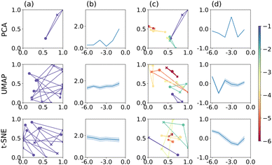 | ||
| Fig. 3 PCA, UMAP, and t-SNE applied to b/w image data. Plots are arranged in the same way as in Fig. 2. | ||
For UMAP and t-SNE, the stochasticity of the outcome is clearly apparent in column (a), centre and bottom, respectively. Both algorithms produce good separation of the three mechanisms for this electrode radius, but the orientation and to some extent size of the triangle (P score) varies, as noted above. Across all electrode radii, their performance is however rather consistent (close to P = 2) and better than for PCA on images. Following hyperparameter optimisation on triplet separation, the latter appears to work best for the smallest electrode radius used here; otherwise the S scores remain close to 0, indicating some overlap between the triplet clusters, columns (c)–(d). Under these conditions, UMAP still appears to be better than t-SNE, with regards to separating the different mechanisms, as for t-SNE the E and EC mechanisms largely seem close together, except for r = 1 × 10⁻² cm (light green triangle in column (c), corresponding P scores not shown).
Finally, we compare PCA, t-SNE and UMAP applied to the feature extractor output of VGG-16. The results are shown in Fig. 4, following the same format as in Fig. 2 and 3. To get an impression of how the feature extractor “sees” the CV image data, we refer the reader to Section S4 in the ESI,† which show examples of how the individual images are represented in the filter output of the feature extractor (before flattening into a 1D output vector). Bright areas are strongly represented and, by implication, have a larger effect on the classification result. These appear to be, by and large, curved regions of the CV or inflection points, rather than the redox-inactive regions at low potentials, for example, and suggests that VGG-16 indeed identifies features that are related to the electrochemical process, rather than the overall appearance of the image.
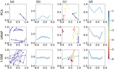 | ||
| Fig. 4 PCA, UMAP, and t-SNE applied to the feature extractor output of VGG-16. Plots are arranged as described in Fig. 2. | ||
Application of PCA, UMAP and t-SNE to the feature extractor output leads to qualitatively similar results, compared to using images directly, both for the separation of individual triplets, column (a), and across the range of electrode radii, column (b). Specifically, PCA appears to perform marginally better, UMAP somewhat worse and t-SNE comparably well and still best comparing the three methods. In terms of the S scores, PCA produces reasonably well separated point triplets, column (c), and, over all electrode radii, a better separation than when applied to image data directly, column (d). The S score reaches values close to 1 for some r-values, even though there does not appear to be an overall trend. Similarly, for UMAP, triplet separation is satisfactory and S scores are on average larger than when applied to image data directly. Finally, t-SNE does not separate the value triplets well with some overlap remaining and S scores close to 0, for all but one radius (r = 1 × 10⁻¹ cm). In other words, t-SNE still reproduces the neighbourhood relation according to mechanism better than electrode radius, leading to good separation within a point triplet, but relatively poor differentiation between them.
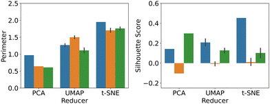
Based on these detailed comparisons, the question arises which methodology and data input format results in the best overall performance, in terms of the respective optimisation target (mechanism vs. electrode radius). Hence, we show the average P- and S scores for dimensionality reduction applied to numerical input data (blue), images (orange) and feature extractor output (green), in Fig. 5. See Fig. S10 in the ESI,† for further information.
In terms of the P score, a fairly consistent picture emerges, namely that all three dimensionality reduction techniques work equally well on the different input formats. PCA and t-SNE appear to work slightly better on numerical input data, while UMAP produced the best result when directly applied to images. Importantly, however, both UMAP and t-SNE clearly outperform PCA in this metric and while PCA has the advantage of being deterministic, not requiring any hyperparameter optimisation and being computationally inexpensive, once optimised, both UMAP and t-SNE feature improved separation performance. Using the feature extractor output did not offer any advantage in this case, but it is nevertheless notable that at least comparable results have been obtained, given that the feature extractor had been trained on unrelated image data and the electrochemically relevant features highlighted in the filter outputs (see ESI†).
With regards to the S score, the picture is rather less clear cut. The best performing methodology here was t-SNE applied to raw numerical data, followed by PCA on features and UMAP on numerical data. Thus, feature extraction appeared to have a significant benefit in this context, even though further analysis may be required to investigate this effect in more detail.
Finally, we also investigated the effect of small to moderate amounts of noise on the classification, see Section S6 in the ESI.† Intuitively, one might expect the differentiation of CV shapes to become more difficult, as there is more likely going to be more overlap between the CV traces, cf. Fig. S11 (ESI†). This expectation is indeed borne out with regards to the separation of the three mechanisms, i.e. the average P score performance, Fig. S12 (left column) (ESI†), where the overall sequence t-SNE > UMAP > PCA is maintained, but P values decrease with increasing amounts of noise (without re-optimising the hyperparameters). For the optimisation towards highest S scores, Fig. S12 (right column) (ESI†) the picture is however more complex. Applied to raw data, the performance of UMAP and PCA remains more or less unchanged as the amount of noise is increased, but interestingly t-SNE does significantly worse when even small amounts of noise are added. When applied to image data, the separation performance slightly increases with increasing noise levels with t-SNE and UMAP performing marginally better than PCA in all cases. When applied to features, t-SNE becomes the best performing method in the presence of noise, followed by PCA and then UMAP. Identifying the origin of some of these effects requires further study and will form part of our future work.
Overall, among the methodologies investigated here and considering both P- and S score performance, in the absence of noise the best performing one appears to be t-SNE applied to raw numerical data. In the presence of noise, t-SNE on features is preferable, followed by UMAP applied to raw data. PCA shows satisfactory performance under all the conditions studied and compared to the other two does not require hyperparameter optimisation. It is however outperformed by some of the other methodologies, highlighting the necessity to carefully consider the dimensionality reduction technique as well as the data input format for a given classification task.
TA designed the study and supervised the work. CW performed the data analysis and co-developed the analysis pipeline. AF produced the electrochemical simulations. AV performed initial tests of approach. All authors contributed to the writing the manuscript.
Conflicts of interest
There are no conflicts to declare.Notes and references
- C. N. Elgrishi, K. J. Rountree, B. D. McCarthy, E. S. Rountree, T. T. Eisenhart and J. L. Dempsey, J. Chem. Educ., 2018, 95, 197–206 CrossRef.
- P. Stonehart and P. N. Ross, Catal. Rev., 1975, 12, 1–35 CrossRef CAS.
- P. N. Ross and J. Lipkoswki, “Electrocatalysis”, in Frontiers of Electrochemistry, Wiley-VCH, 1998 Search PubMed.
- P. Kissinger and W. R. Heineman, Laboratory Techniques in Electroanalytical Chemistry, Marcel Dekker, Inc., New York, 1996 Search PubMed.
- R. G. Compton and C. E. Banks, Understanding Voltammetry, Imperial College Press, 2010 Search PubMed.
- E. J. F. Dickinson, H. Ekstrom and E. Fontes, Electrochem. Comm., 2014, 40, 71–74 CrossRef CAS.
- D. Godfrey, J. H. Bannock, O. Kuzmina, T. Welton and T. Albrecht, Green Chem., 2016, 18, 1930–1937 RSC.
- M. Sylvain, F. Lehoux, S. Morency, F. Faucher, E. Bharucha, D. M. Tremblay, F. Raymond, D. Sarrazin, S. Moineau, M. Allard, J. Corbeil, Y. Messaddeq and B. Gosselin, IEEE Trans. Biomed. Circ. Syst., 2018, 12, 1289–1300 Search PubMed.
- O. J. Wahab, M. Kang, E. Daviddi, M. Walker and P. R. Unwin, ACS Catal., 2022, 12, 6578–6588 CrossRef CAS PubMed.
- N. Markovic and P. N. Ross, Langmuir, 1993, 9, 580–590 CrossRef CAS.
- Y. Garsany, O. A. Baturina, K. E. Swider-Lyons and S. S. Kocha, Anal. Chem., 2010, 82, 6321–6328 CrossRef CAS PubMed.
- W. S. R. Teixeira, M. K. L. Silva, D. Grasseschi, C. A. Senna, A. Guimarães de Oliveira, J. Gruber, I. Cesarino and M. Oliveira Salles, J. Electrochem. Soc., 2022, 169, 047526 CrossRef.
- D. Ortiz-Aguayo, K. De Wael and M. del Valle, J. Electrochem. Soc., 2021, 169, 115770 Search PubMed.
- S. Acharya, D. Das, T. N. Chatterjee, S. Mukherjee, R. Banerjee Roy, B. Tudu and R. Bandyopadhyay, IEEE Sens. J., 2021, 21, 20589–20595 CAS.
- J. M. Díaz-Cruz, R. Tauler, B. S. Grabarić and M. E. E. Casassas, J. Electroanal. Chem., 1995, 393, 7–16 CrossRef.
- G. Hinton and S. Roweis, Advances in Neural Information Processing Systems, 2002, vol. 15 Search PubMed.
- L. Van Der Maaten and G. Hinton, J. Mach. Learn. Res., 2008, 9, 2579–2605 Search PubMed.
- L. McInnes, J. Healy and J. Melville, arXiv, 2020, preprint, arXiv:1802.03426v3 [stat.ML] DOI:10.48550/arXiv:1802.03426v3.
- T. Sainburg, L. McInnes and T. Q. Gentner, Neural Comput., 2020, 33, 2881–2907 Search PubMed.
- T. Albrecht, G. Slabaugh, E. Alonso and S. M. R. Al-Arif, Nanotechnology, 2017, 28, 423001 CrossRef PubMed.
- G. F. Kennedy, J. Zhang and A. M. Bond, Anal. Chem., 2019, 91, 12220–12227 CrossRef CAS PubMed.
- L. Gundry, G. Kennedy, A. M. Bond and J. Zhang, Faraday Discuss., 2022, 233, 44–57 RSC.
- J. X. Zhang, B. Yordanov, A. Gaunt, M. X. Wang, P. Dai, Y.-J. Chen, K. Zhang, J. Z. Fang, N. Dalchau, J. Li, A. Phillips and D. Y. Zhang, Nat. Commun., 2021, 12, 4387 CrossRef CAS PubMed.
- K. Simonyan and A. Zisserman, 3rd Int. Conf. Learn. Represent. ICLR 2015-Conf. Track Proc. DOI:10.48550/arxiv.1409.1556.
- A. Vladyka and T. Albrecht, Mach. Learn. Sci. Technol., 2020, 1, 035013 CrossRef.
- A. Krizhevsky, I. Sutskever and G. E. Hinton, NIPS’12: Proc. 25th Int. Conf. on Neural Information Processing Systems 2012, 1, 1097–105.
- Y. Wei, Y. Sun and X. Tang, J. Phys. Chem., 1989, 93, 4878–4881 CrossRef CAS.
- D. M. Mohilner, R. N. Adams and W. J. Argersinger, J. Am. Chem. Soc., 1962, 84, 3618–3622 CrossRef CAS.
Footnote |
| † Electronic supplementary information (ESI) available. See DOI: https://doi.org/10.1039/d2cc03187f |
| This journal is © The Royal Society of Chemistry 2022 |

