 Open Access Article
Creative Commons Attribution 3.0 Unported Licence
Salient space detection algorithm for signal extraction from contaminated and distorted spectrum
Y. W.
Jia
 ab,
S. Y.
Sun
a,
L.
Yang
a and
D.
Wang
c
aSchool of Mechanical Engineering, Tianjin University of Technology, China. E-mail: yunweijia@tjut.edu.cn
bTianjin Key Laboratory of the Design and Intelligent Control of the Advanced Mechatronical System, China
cSchool of Computer Science and Engineering, Tianjin University of Technology, China
First published on 14th May 2018
Abstract
An algorithm for signal extraction from a contaminated and distorted spectrum is proposed. First, this algorithm combines the salient space of the spectrum and the statistical characteristics of the noise to detect signal regions at different scales. Second, it extracts signals by subtracting the baseline from the spectrum in the signal regions. The baseline is fitted by segmented polynomial functions. This algorithm has been applied to simulated and experimental data, and the results show that this algorithm can accurately and automatically extract signals with varying widths from a contaminated spectrum. This method minimizes the influence of baseline distortion and exhibits good anti-noise capability and high real-time performance.
1 Introduction
A spectrum can be used to extract information from a sample such as the chemical and physical structure of a material,1,2 or the concentration of a solution.3,4 Spectrum is widely used in many fields such as mass spectrometry and chromatography. However, random noises and irregular baseline distortions, which can arise from several hardware and processing sources, inevitably exist in the spectrum.5 These interferences in a spectrum result in incorrect detection of signal regions (representing the structural information of the sample) and inaccurate calculation of signal intensity6,7 (denoting the concentration of the sample). Thus, it is important to avoid the influence of these interferences to correctly and accurately extract signals from the spectrum.8Many methods have been used to extract signals such as the zero-crossing technique9 (searching for zeros in the first derivative and treating these positions as signal regions), thresholding algorithm6,7 (where only points three times larger than the standard deviation of the spectrum noise are treated as signal points) or wavelet decomposition and integration.10–13 All these methods have significantly contributed to signal extraction. The zero-crossing technique is the simplest method to extract signals, but it is invalid when noises exist.9 Thresholding algorithm is one of the mainstream approaches in signal extraction because of its simplicity and anti-noise capability. However, two issues must be addressed. First, weak signals, having peaks three times smaller than the standard deviation of the spectrum noise, are lost in the spectrum. Second, the accuracy of this approach is adversely affected by the baseline, and this approach may fail because baseline distortions can be significantly larger than peak intensities.6 Wavelet decomposition is widely used to eliminate baseline rolling before the thresholding algorithm or even to directly extract signals.14 However, its accuracy is often influenced by the wavelet base and the number of decompositions, which are often chosen by experience, thereby restricting its applicability.15,16
In several literatures, the baseline is corrected before signal extraction to reduce baseline influence.17 However, baseline correction of the whole spectrum is difficult, and it increases the computational problem. Furthermore, many methods must remove signal regions before baseline correction to acquire a better baseline.6 Thus, baseline correction and signal extraction are typically restricted by each other.18
Algorithms that do not use a model of the baseline or signal shape and that have anti-noise capability are preferred. Many iterative algorithms19–21 and Difference-of-Gaussian (DoG) functions can meet this requirement. Adaptive iteratively reweighted penalized least squares (airPLS) is a well-known iterative algorithm, because it is flexible and valid; however, it needs further optimization. Lowe22,23 proposed DoG for image processing, and it has also been used for signal extraction.24 Furthermore, DoG can automatically extract signals of different widths in the same spectrum, and its accuracy is seldom influenced by baseline and noise. However, applying DoG is time consuming.
Herein, we propose Salient-Space-Detection algorithm (SSD) for signal extraction. SSD has been developed with reference to DoG and noise statistics. SSD has all of the advantages of DoG, and it gives more real-time and accurate results than other algorithms.
We have evaluated our method using simulated spectra, and we have applied it to real measured spectra. The results show that the algorithm is robust, real-time and accurate for signal extractions of different kinds of spectra.
2 Methods
2.1 Signal region detection
Signal region detection based on SSD can be represented as follows:First, the background space of a spectrum is defined as a function, B(x, r), obtained by averaging the offset spectrum, I(x − r) and I(x + r), of the original input spectrum, I(x).
| B(x, r) = [I(x − r) + I(x + r)]/2 | (1) |
Here, r is the offset value of the original spectrum, which also represents the scale of the background spectrum. Different values of r produce various background spectra. All background spectra constitute the background space.
Second, the salient space, H(x, r), can be obtained from the difference of the original spectrum and background space.
 | (2) |
Here, a positive spectrum is a spectrum, such as a Raman spectrum, having peaks larger than the baseline. A negative spectrum is a spectrum, such as an absorption spectrum, having peaks smaller than the baseline.
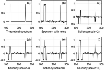
As shown in Fig. 1a, the half-breadths of the square signal and the sharp Gaussian signal are 8 and 4 points, respectively (the width of a signal was defined as the total number of points having amplitude that is 1% larger than the maximum amplitude of this signal). Salient space, which can be obtained by eqn (2), is shown in Fig. 1b–f. When the scale of the salient space conforms to the half-breadth of the signal, the result of H(x, r) reaches its maximum at the centre of the signal region. Thus, detecting the maximum of H(x, r) can help derive signals with different widths.
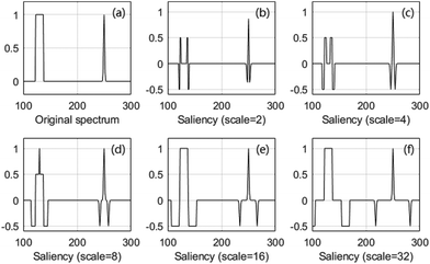 | ||
| Fig. 1 Saliency of typical salient space. The horizontal and vertical axes of (b)–(f) represent position and saliency, respectively. | ||
Next, the central coordinates of signal regions, Xsc, and the half-breadth of signal regions, Rs, are obtained by detecting the maximum of H.
 | (3) |
Here, Δr is the difference of two nearby scales.
Noises are neglected in eqn (3). When noises are existed, as shown in Fig. 2, the maximum of H(x, r) is not guaranteed to be at the centre of the signal region even if the scale of salient space conforms to the half-breadth of the signal.
 | ||
| Fig. 2 Noise influence. The maximum saliency of the square signal is not at the centre of the signal and is not obtained when the scale equals half-breadth. | ||
The most common method to decrease the influence of noise is denoising. However, most denoising methods inevitably weaken the signal intensity and induce spectrum distortion. Thus, we choose to revise eqn (3) instead of denoising the original spectrum before SSD.
First, the absolute mean of the noises, μr, of each scale of the salient space is calculated. All points larger than kμr and the mean value of the d neighbourhoods larger than μr are then treated as candidate points of signal regions.
 | (4) |
 | (5) |
Here, Nh is the total number of points in H(x, r), and k and d are constants; their values can be set as 2 and 4, respectively (these values correspond to the confidence level of 99% under normal distribution).
If only signal regions with peaks clearly larger than the noise can be detected, then k can be set at a value larger than 3, and eqn (5) can be simplified as eqn (6).
| Xts = {x|H(x, r) > kμr} | (6) |
Next, the start and end coordinates, Xs and Xe, of the signal regions are obtained by eqn (7) and (8), respectively.
| Xs = {(x1 − rT)∪(xj − rT)|xj − xj−1 > rT j∈(2, Ns)}, | (7) |
| Xe = {(xj + rT)∪(xNs + rT)|xj+1 − xj > rT j∈(1, Ns − 1)}. | (8) |
Here, xj represents the candidate signal points, Ns is the total number of these points, and x1 and xNs are the first and the last candidate signal points, respectively. rT is a threshold, and it should be set at 3Δr to get good results.
2.2 Signal extraction
Once the signal regions are detected, only the baseline of the signal regions is necessary to extract the signals. Thus, we cut the baseline into many segments, and we fitted each segment separately. Despite many baseline fitting algorithms, such as linear interpolation,6 iterative moving averaging,25 and Whittaker Smoother,26 we choose a lower-order polynomial function27 to fit the baseline. This choice is attributed to the smooth, real-time polynomial fitting while showing fidelity to the original data when the spectrum is divided into many segments.First, a certain number of neighbour points of a signal region are chosen. Second, the baseline of this signal region is fitted by a lower-order polynomial function using the chosen points. Finally, signals can be extracted by subtracting the baseline from the spectrum at signal regions.
3 Experimental
We applied the algorithm to various spectra, including simple simulated spectra with constructed data, complex simulated spectra with absorption data, Nuclear Magnetic Resonance (NMR) data, real absorption spectra obtained by experiments and real Raman spectra from the Handbook of Minerals Raman Spectra database,28 to evaluate its performance.Simulated spectra were used because their theoretical signal regions and intensities were known; thus, evaluating the accuracy of the algorithm was easy. Real spectra were utilised because they can indicate the effect of an algorithm in real applications.
3.1 Simple simulated data
Simple simulated data were employed because they can show the process and results clearly.All simulated spectra can be expressed as follows:
| s(x) = a(x) + n(x) + b(x). | (9) |
Here, a(x) is the theoretical signal, n(x) is the Gaussian noise, b(x) is the theoretical baseline and s(x) is the simulated spectrum.
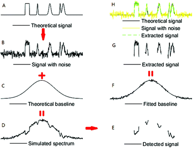
More than 20![[thin space (1/6-em)]](https://www.rsc.org/images/entities/char_2009.gif) 000 spectra were simulated with various SNRs (signal-to-noise ratios) and SBRs (signal-to-baseline ratios) to evaluate SSD performance. A Gaussian curve was used as the theoretical baseline in these spectra. The Gaussian curve used was typical; it had abundant curvatures in a single line. Four typical signals were constructed to enhance the simulation: one square signal, one sharp Gaussian signal, one broad Gaussian signal and one substantially overlapped signal. Fig. 3 shows the entire process; SNR and SBR used in this example were 30 and 0.2, respectively.
000 spectra were simulated with various SNRs (signal-to-noise ratios) and SBRs (signal-to-baseline ratios) to evaluate SSD performance. A Gaussian curve was used as the theoretical baseline in these spectra. The Gaussian curve used was typical; it had abundant curvatures in a single line. Four typical signals were constructed to enhance the simulation: one square signal, one sharp Gaussian signal, one broad Gaussian signal and one substantially overlapped signal. Fig. 3 shows the entire process; SNR and SBR used in this example were 30 and 0.2, respectively.
3.2 Complex simulated data
Spectra, such as real absorption and real NMR spectra, containing large amounts of data were simulated.From the HITRAN spectroscopic database,29 we can obtain the absorption intensity coefficient, a(v), of C2H2. We chose the coefficient larger than 0.0059 × 10⁻¹⁹ as pure absorption peak, multiplied it by 5 × 10¹⁹ and designed each peak as Gaussian distribution. Thus, we derived the pure absorption spectrum, a(x). The spectrum length was designed as 7200 sample points, mimicking that of the C2H2 experimental spectra. Noise was then added to the pure absorption spectrum. Finally, the spectrum with noise was added to the theoretical baseline. The theoretical baseline, b(x), was set as a slash connected with a Gaussian curve. This kind of baseline has abundant curvature, and it is more typical than a Gaussian curve.
The simulated NMR spectrum was extracted from the real NMR spectrum offered by Qingjia Bao.7 First, we used DoG to detect the signal regions of real spectrum. Second, we fitted the baseline based on segmented lower-order polynomial fitting and segmented kernel smoothing.22 Third, we extracted the signals as theoretical spectrum by subtracting the baseline from the real spectrum at signal regions. Finally, we added the noise and theoretical spectrum to the theoretical baseline, with its theoretical baseline, b(x), set as a slash connected with a Gaussian curve.
3.3 Real absorption data
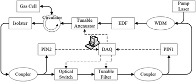
The efficiency of the SSD algorithm was also evaluated by C2H2 absorption spectrum. The gas sensing system we used was an intra-cavity fibre ring laser gas sensing system (Fig. 4). The system consisted of an EDFA pumped by a 980 nm diode laser, a variable attenuator, a circulator, a gas cell with reflector, an isolator, a fibre coupler, and a Fabry–Perot tunable filter (TF), and its transmission wavelength was controlled by the controlling voltage from data acquisition equipment (DAQ); the system also consisted of two InGaAs PIN photodetectors with an operating wavelength of 1000–1650 nm and a DAQ of NI-USB-6251. The EDFA wavelength region was 1525–1565 nm. The bandwidth and the free spectral range of TF were 0.0353 and 200 nm, respectively. The length of the gas cell was 20 cm, and the gas concentration was 1%.We utilised the amplified absorption intensity coefficient, a(v), as the theoretical intensity in the experiments.
3.4 Real Raman data
Real Raman spectral data were obtained from the Handbook of Minerals Raman Spectra database. These real spectra have different SNRs and baselines. We chose three typical spectra, i.e., spectra of adamite, fluorliddicoatite and abelsonite. The baseline of adamite is similar to a Gaussian curve connected with a slash. The baselines of fluorliddicoatite and abelsonite are more complex. These three spectra simultaneously have sharp, broad, strong and weak signals. Additionally, these spectra have signals that overlap with each other. The corresponding processed spectra were also given in the database. We used the processed spectra as the criteria for our comparison of SSD, DoG and airPLS.4 Results and discussion
4.1 Influences of SNR and SBR
The influences of SNR and SBR were studied using simple simulated data. Table 1 shows that the accuracy of SSD was influenced by SNR and SBR in the following ways. (1) When SNR and SBR were smaller than 20 and 0.5, respectively, signal extraction may fail; otherwise, signals can be extracted all the time. (2) As SNR and SBR increased, the standard derivation of power error always decreased, whereas the mean error sometimes oscillated if SNR was smaller than 50. (3) When SNR was smaller than 50, the mean and standard derivation of power error worsened rapidly as the SNR decreased; otherwise, they were almost stable and had high accuracies. The largest mean and standard derivation values were 1.1% and 3.3%, respectively. (4) The change in the accuracy with SNR was larger than that with SBR.| P1 | P2 | P3 | P4 | ||||||||||||||||||
|---|---|---|---|---|---|---|---|---|---|---|---|---|---|---|---|---|---|---|---|---|---|
| 0.2 | 0.3 | 0.5 | 0.75 | 1 | 0.2 | 0.3 | 0.5 | 0.75 | 1 | 0.2 | 0.3 | 0.5 | 0.75 | 1 | 0.2 | 0.3 | 0.5 | 0.75 | 1 | ||
| 20 | mean | Non | Non | Non | −2.1 | −0.1 | Non | Non | Non | −1.3 | −0.6 | Non | Non | Non | −0.7 | −1.1 | Non | Non | Non | −2.1 | 0.7 |
| Std | Non | Non | Non | 12.1 | 9.0 | Non | Non | Non | 12.2 | 9.5 | Non | Non | Non | 11.0 | 8.9 | Non | Non | Non | 12.8 | 9.3 | |
| 30 | mean | −0.6 | −0.6 | 0.1 | −0.9 | 0.2 | −1.0 | 0.2 | 0.4 | −0.6 | −0.2 | −1.0 | 0.6 | −0.4 | −0.1 | −0.3 | 0.4 | 0.8 | 0.4 | 0.0 | −0.1 |
| Std | 15.0 | 9.3 | 6.4 | 4.1 | 3.3 | 13.7 | 10.3 | 6.7 | 4.1 | 3.2 | 14.8 | 10.7 | 6.2 | 4.0 | 3.3 | 13.5 | 10.6 | 5.9 | 4.0 | 3.3 | |
| 50 | mean | 1.0 | 0.7 | 0.4 | 0.1 | 0.0 | 1.1 | 0.5 | 0.3 | 0.1 | 0.1 | 1.1 | 0.6 | 0.3 | 0.1 | 0.1 | 1.0 | 0.6 | 0.3 | 0.1 | 0.0 |
| Std | 3.3 | 2.2 | 1.4 | 1.0 | 0.0 | 3.3 | 2.2 | 1.4 | 1.0 | 0.0 | 3.3 | 2.2 | 1.0 | 1.0 | 0.0 | 3.3 | 2.2 | 1.0 | 1.0 | 0.0 | |
| 75 | mean | 1.1 | 0.6 | 0.3 | 0.1 | 0.1 | 1.1 | 0.6 | 0.3 | 0.1 | 0.1 | 1.1 | 0.6 | 0.3 | 0.1 | 0.1 | 1.1 | 0.6 | 0.3 | 0.1 | 0.1 |
| Std | 3.0 | 2.0 | 1.0 | 0.0 | 0.0 | 3.0 | 2.0 | 1.0 | 0.0 | 0.0 | 3.0 | 2.0 | 1.0 | 0.0 | 0.0 | 3.0 | 2.0 | 1.0 | 0.0 | 0.0 | |
| 100 | mean | 1.1 | 0.6 | 0.3 | 0.1 | 0.1 | 1.1 | 0.6 | 0.3 | 0.1 | 0.1 | 1.1 | 0.6 | 0.3 | 0.1 | 0.1 | 1.1 | 0.6 | 0.3 | 0.1 | 0.1 |
| Std | 3.0 | 2.0 | 1.0 | 0.0 | 0.0 | 3.0 | 2.0 | 1.0 | 0.0 | 0.0 | 3.0 | 2.0 | 1.0 | 0.0 | 0.0 | 3.0 | 2.0 | 1.0 | 0.0 | 0.0 | |
The statements (1), (2) and (3) indicate that SSD has strong anti-noise and anti-baseline-distortion capability; however, its accuracy and stability are still influenced by noise and baseline distortion. Thus, SSD cannot be used only when both SNR and SBR are too small. The statements (2), (3) and (4) indicate that the influence of SNR is larger than that of SBR and thus, improving the denoising performance may be important for future studies.
SBR and power error are defined as follows:
 | (10) |
 | (11) |
Here, n is the number of extracted signal points, aE(xi) is the intensity of the extracted signal and a(xi) is the intensity of the theoretical signal.
4.2 Comparison with other algorithms
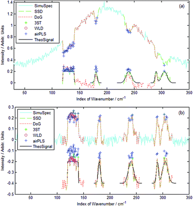
Fig. 5 shows the signal region detection results of two simple simulated spectra. SimuSpec and TheoSignal represent the simulated spectrum and theoretical signals, respectively, SSD represents the proposed algorithm, DoG denotes the DoG algorithm, 3ST represents the thresholding algorithm, WLD denotes wavelet decomposition combined with the thresholding algorithm and airPLS denotes airPLS combined with the thresholding algorithm. Of all the detected signal regions, the one detected by SSD is the most accurate, regardless of whether the theoretical baseline is chosen as a Gaussian curve or a horizontal line and regardless of whether the signal is negative or positive. Please note that in Fig. 5a, no signal points were detected by 3ST or WLD. However, the above-mentioned comparison is only based on a contaminated spectrum. A good result can also be obtained by 3ST when the baseline is a horizontal line and SNR is high.DoG and airPLS were used to compare with SSD in the next experiments because they are more accurate than 3ST and WLD.
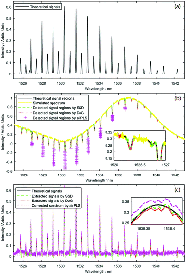 | ||
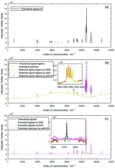
| Fig. 6 Simulated data of C2H2 absorption spectrum: (a) theoretical spectrum, (b) signal region detection and (c) signal extraction. | ||
DoG has denoising capability because it obtains its scale space by convolution, as shown in eqn (12). Convolution, like a smooth filter, is influenced by the convolution radius. When the radius is too small, it cannot eliminate the noise, and some noise points, such as those at about 1526.1 and 1533.6 nm, may be treated as signal points, as shown in Fig. 6b. If the radius is too large, some signal points, such as that at about 1526.7 nm, are reduced and treated as baseline points, as shown in Fig. 6b.
| D(x, σ) = (G(x, kσ) − G(x, σ)) * I(x). | (12) |
Here, G(x, kσ) and G(x, σ) are the variable-scale Gaussian functions, σ is in proportion to the convolution radius, I(x) is the original input spectrum and D(x, σ) is the Difference-of-Gaussian. By detecting the maximum or minimum of D(x, σ) in various scale spaces, we can detect signals with various widths.
SSD uses noise statistics, as shown in eqn (4) and (5), to decrease the influence of noise. Additionally, SSD is not affected by the baseline or scale of salient space, and its confidence level is larger than 99%. Thus, SSD is more accurate than DoG.
AirPLS can correct the spectrum, but neither its signal region detection nor intensity accuracy is as good as those of SSD or DoG, as shown in Fig. 6b and c; this is because airPLS does not have strong anti-noise capacity, and the anti-baseline-distortion capability is not as good as is supposed.
Fig. 7 presents the results of a simulated NMR spectrum. The analysis is omitted here for briefness because the phenomena of Fig. 7 are the same as those of Fig. 6. Thus, we can conclude that SSD is more accurate than DoG, and DoG is more accurate than airPLS.
4.3 Real absorption data
An example of a C2H2 absorption spectrum showing a poor baseline and broad, contaminating peaks is depicted in Fig. 8a. SSD accurately extracts the signal regions even when the original spectrum is distorted sharply near 1526 nm. As Fig. 8b shows, all signal regions are extracted accurately by SSD, and no false-positive or false-negative observations are observed. The results are in accordance with the simulation results of Fig. 6, with the exception of intensity.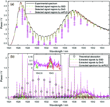 | ||
| Fig. 8 Experimental data of C2H2 absorption spectrum: (a) signal region detection and (b) signal extraction. | ||
Many factors, such as existing noise and inaccurately extracted baseline, can induce the intensity difference between the theoretical and extracted spectra. However, the most important reason is that the spectrum is obtained by the intracavity fibre ring laser gas sensing system. In this system, the absorption length, L, is not absolutely identical because of the difference in the laser's settling time at various wavelengths (the larger the settling time, the longer the absorption length). Although the concentration, c, is a constant, the product of c × L differs at various wavelengths. Thus, the proportions of the real absorption intensity, K, and absorption intensity coefficient, a(v), are not the same by Lambert–Beer law as follows:
| c = K/(a(v) × L) ⇒ c × L = K/a(v). | (13) |
Using the same intracavity fibre ring laser gas sensing system, the settling time, ts, of large absorption peaks is found to be shorter than that of the small absorption peaks of both sides. The settling time of large absorption peaks near 1530 nm is the shortest and then, it increases slightly as the wavelength increases. Considering L = v × ts, we can say that the proportion, K/a(v), of large absorption peaks should be smaller than that of the small absorption peaks of both sides. The proportion, K/a(v), of large absorption peaks near 1530 nm should be the smallest, and it should increase slightly with the increase in the distance between the wavelength of the peak and 1530 nm. Fig. 8 shows this deduction.
From Fig. 8 and the analysis mentioned above, we can see that SSD can extract signals from real absorption data, and the result of SSD is better than that of DoG or airPLS.
4.4 Real Raman data
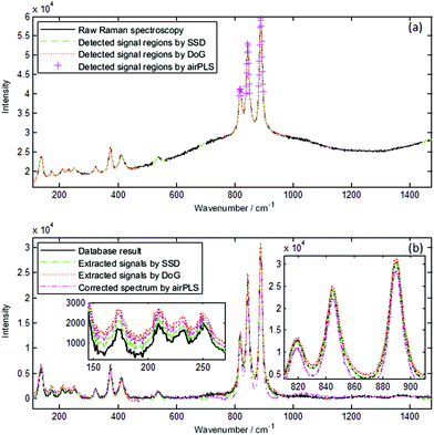
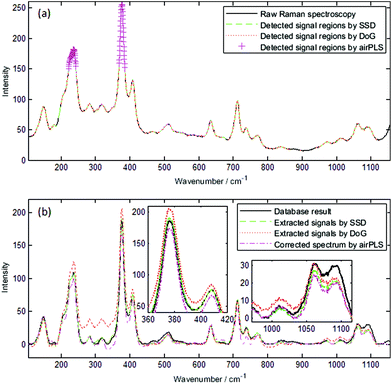
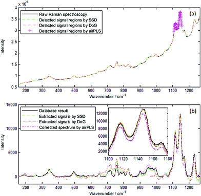
Fig. 9 presents the results of adamite spectrum. The extracted signals obtained by SSD concur with the processed results of the dataset, especially for the signals between 800 and 950 cm−1. Near 200 cm−1, the extracted signal is slightly larger than the database result, but it is still more accurate than the results obtained by DoG and airPLS.The raw spectra of fluorliddicoatite and abelsonite are even more complex than the adamite spectrum, and identifying where baseline and signals are located, even manually, is difficult. The fluorliddicoatite result obtained by SSD almost concurs with the database result, and it is more accurate than the results obtained by DoG and airPLS. The abelsonite result is not as good as the adamite or fluorliddicoatite result; however, it is better than the result obtained by DoG or airPLS. Fig. 11b shows that the intensity data near 750 and 1210 cm−1 obtained by SSD are less accurate than the results obtained by airPLS; however, the results of SSD are better than those of airPLS or similar with those of airPLS at other wavenumber s. The results obtained by DoG are the least accurate for the abelsonite spectrum. Thus, SSD is the most effective method for the signal extraction of Raman spectra.
SSD is more accurate than DoG and airPLS due to the same reasons mentioned in section 4.2. AirPLS does not have strong anti-noise capability, and the anti-baseline-distortion capability is not as good as is supposed. DoG has strong anti-noise and anti-baseline-distortion capability; however, its convolution radius may influence the signal region detection.
Fig. 9–11 also illustrate that the overlapping of the signals may influence the accuracy of the intensity of the extracted signals, but Table 1 does not show this phenomena. When many signals overlap with each other and combine to form a signal that is too broad, such as the signal near 200 cm−1 of Fig. 9 and the signal near 750 cm−1 of Fig. 11, some signal points may be treated as baseline points. Thus, the accuracy of the fitted baseline declines and ultimately influences the accuracy of the intensity of these signals. Apart from that, the intensity of the extracted signals is accurate and is not influenced by the signal and baseline shapes.
5 Conclusions
We proposed an SSD algorithm for signal extraction. Experimental results showed that the new algorithm is effective for most kinds of spectra such as absorption, NMR and Raman spectra. Three main improvements were obtained by using this algorithm. First, SSD could automatically and accurately extract signals even if the spectrum contained broad and sharp peaks synchronously with noise. Second, SSD could minimize the influence of the baseline distortion. Lastly, the proposed algorithm exhibited high real-time performance because it did not require iteration or convolution. The time for signal region detection was only 0.011 s. The total time for signal extraction was only about 0.031 s. We showed that SSD is an enhanced signal extraction method in which the results were not influenced by the baseline or signal shape, and it exhibited anti-noise capability and better real-time performance. Since the SNR value still influenced the accuracy of the extraction result when SNR was smaller than 50, the improvement of the denoising performance is considered in our following studies.Conflicts of interest
There are no conflicts to declare.Acknowledgements
This study was supported in part by the National Natural Science Foundation of China under Grant 61201081.The authors thank Juntao Liu and Bingqiang Liu for their support on the Raman data.
References
- S. L. Ye and E. Aboutanios, Efficient Peak Extraction of Proton NMR Spectroscopy Using Lineshape Adaptation, IEEE Int. Conf. Acoust. Speech Signal Process.,, 2014, 5661–5665 Search PubMed
.
- J. Liu, J. Sun, X. Huang, G. Li and B. Liu, Goldindec: A Novel Algorithm for Raman Spectrum Baseline Correction, Appl. Spectrosc., 2015, 69, 834–842 CrossRef PubMed
.
- M. D'Addario, D. Kopczynski, J. I. Baumbach and S. Rahmann, A Modular Computational Framework for Automated Peak Extraction from Ion Mobility Spectra, BMC Bioinf., 2014, 15, 25 CrossRef PubMed
.
- M. Li, J. M. Dai, K. Liu and G. D. Peng, Performance Analysis and Design Optimization of An Intracavity Absorption Gas Sensor Based on Fiber Ring Laser, J. Lightwave Technol., 2011, 29(24), 3748–3756 CrossRef
.
- H. Seifi, S. Masoum and S. Seifi, Performance Assessment of Chemometric Resolution Methods Utilized for Extraction of Pure Components from Overlapped Signals in Gas Chromatography-Mass Spectrometry, J. Chromatogr. A, 2014, 1365, 173–182 CrossRef PubMed
.
- F. Xian, Y. E. Corilo, C. L. Hendrickson and A. G. Marshall, Baseline Correction of Absorption-Mode Fourier Transform Ion Cyclotron Resonance Mass Spectrum, Int. J. Mass Spectrom., 2012, 325(4), 62–67 Search PubMed
.
- Q. J. Bao, J. W. Feng, F. Chen, W. P. Mao, Z. Liu, K. W. Liu and C. Y. Liu, A New Automatic Baseline Correction Method Based on Iterative Method, J. Magn. Reson., 2012, 218(5), 35–43 CrossRef PubMed
.
-
D. A. Wright, Methods of Automated Spectral Peak Detection and Quantification Having Learning Mode, United States Patent, US8428889B2, 2013 Search PubMed
.
- R. Rodríguez, A. Mexicano, J. Bila, S. Cervantes and R. Ponce, Feature Extraction of Electrocardiogram Signals by Applying Adaptive Threshold and Principal Component Analysis, J. Appl. Res. Technol., 2015, 13(2), 261–269 CrossRef
.
- H. Asfour, L. M. Swift, N. Sarvazyan, M. Doroslovacki and M. W. Kay, Signal Decomposition of Transmembrane Voltage-Sensitive Dye Fluorescence Using Multiresolution Wavelet Analysis, IEEE Trans. Biomed. Eng., 2011, 58(7), 2083–2093 CrossRef PubMed
.
- P. Indic and J. Narayanan, Wavelet Based Algorithm for The Estimation of Frequency Flow from Electroencephalogram Data During Epileptic Seizure, Clin. Neurophysiol., 2011, 122(4), 680–686 CrossRef PubMed
.
- S. Siuly and Y. Li, Designing A Robust Feature Extraction Method Based on Optimum Allocation and Principal Component Analysis for Epileptic EEG Signal Classification, Comput. Methods Prog. Biomed., 2015, 119(1), 29–42 CrossRef PubMed
.
- C. G. Bertinetto and T. Vuorinen, Automatic Baseline Recognition for The Correction of Large Sets of Spectra Using Continuous Wavelet Transform and Iterative Fitting, Appl. Spectrosc., 2014, 68(2), 155–164 CrossRef PubMed
.
- F. Qian, Y. H. Wu and P. Hao, A fully automated algorithm of baseline correction based on wavelet feature points and segment interpolation, Opt. Laser Technol., 2017, 96, 202–207 CrossRef
.
- S. K. Lau, P. Winlove, J. L. Moger, O. L. Champion, R. W. Titball, Z. H. Yang and Z. R. Yang, A Bayesian Whittaker-Henderson Smoother for General-Purpose and Sample-Based Spectral Baseline Estimation and Peak Extraction, J. Raman Spectrosc., 2012, 43(9), 1299–1305 CrossRef
.
- J. C. Cobas, M. A. Bernstein, M. M. Pastor and P. G. Tahoces, A New General-Purpose Fully Automatic Baseline-Extraction Procedure for 1D and 2D NMR Data, J. Magn. Reson., 2006, 183(1), 145–151 CrossRef PubMed
.
- D. Kopczynski and S. Rahmann, An Online Peak Extraction Algorithm for Ion Mobility Spectrometry Data, Algorithms Mol. Biol., 2015, 10, 17 CrossRef PubMed
.
- Q. J. Han, Q. Xie, S. L. Peng and B. K. Guo, Simultaneous spectrum fitting and baseline correction using sparse representation, Analyst, 2017, 142(13), 2460–2468 RSC
.
- H. Liu, Z. Zhang, S. Liu, L. Yan, T. Liu and T. Zhang, Joint Baseline-Correction and Denoising for Raman Spectra, Appl. Spectrosc., 2015, 69(9), 1013–1022 CrossRef PubMed
.
- H. Fu, H. Li, Y. Yu, B. Wang, P. Lu, H. Cui, P. Liu and Y. She, Simple Automatic Strategy for Background Drift Correction in Chromatographic Data Analysis, J. Chromatogr. A, 2016, 1449, 89–99 CrossRef PubMed
.
- M. Koch, C. Suhr, B. Roth and M. M. Wollweber, Iterative Morphological and Mollifier-Based Baseline Correction for Raman Spectra, J. Raman Spectrosc., 2016, 48, 336–342 CrossRef
.
-
D. G. Lowe, Object Recognition from Local Scale-Invariant Features, in Proc. 7th IEEE Int. Conf. Computer Vision, 1999, pp. 1150–1157 Search PubMed
.
- D. G. Lowe, Distinctive Image Features from Scale-Invariant Keypoints, Int. J. Comput. Vision, 2004, 60(2), 91–110 CrossRef
.
- Y. W. Jia, T. G. Liu, K. Liu, L. Zhang and L. Yu, An Automatic Baseline Extraction Algorithm for Intensity Absorption Type Gas Sensing, J. Lightwave Technol., 2013, 31(22), 3582–3587 CrossRef
.
- B. D. Prakash and Y. C. Wei, A Fully Automated Iterative Moving Averaging (AIMA) Technique for Baseline Correction, Analyst, 2011, 136(15), 3130–3135 RSC
.
- O. Devos, N. Mouton, M. Sliwa and C. Ruckebusch, Baseline Correction Methods to Deal with Artifacts in Femtosecond Transient Absorption Spectroscopy, Anal. Chim. Acta, 2011, 705, 64–71 CrossRef PubMed
.
- F. Gan, G. H. Ruan and J. Y. Mo, Baseline Correction by Improved Iterative Polynomial Fitting with Automatic Threshold, Chemom. Intell. Lab., 2006, 82, 59–65 CrossRef
.
- Laboratoire de géologie de Lyon. Handbook of Minerals Raman Spectra [database], ENS-Lyon France, 2000–2015. http://www.geologie-lyon.fr/Raman/, (accessed July 2017).
- L. S. Rothman,
et al., HITRAN Molecular Spectroscopic Database, J. Quant. Spectrosc. Radiat. Transfer, 2004, 96, 139–204 CrossRef
, (accessed July 2013).
| This journal is © The Royal Society of Chemistry 2018 |

