 Open Access Article
Chemometrics for ion mobility spectrometry data: recent advances and future prospects
Ewa
Szymańska
ab,
Antony N.
Davies
cd and
Lutgarde M. C.
Buydens
*a
aRadboud University, Institute for Molecules and Materials, P.O. Box 9010, 6500 GL Nijmegen, The Netherlands. E-mail: chemometrics@science.ru.nl; Fax: +31-24-3652653; Tel: +31-24-3653192
bTI-COAST, Science Park 904, 1098 XH Amsterdam, The Netherlands
cSchool of Applied Sciences, Faculty of Computing, Engineering and Science, University of South Wales, Pontypridd, CF37 1DL, UK
dAkzoNobel Chemicals bv Strategic Research Group – Measurement & Analytical Science, P.O. Box 10, 7400 AA, Deventer, The Netherlands
First published on 1st August 2016
Abstract
Historically, advances in the field of ion mobility spectrometry have been hindered by the variation in measured signals between instruments developed by different research laboratories or manufacturers. This has triggered the development and application of chemometric techniques able to reveal and analyze precious information content of ion mobility spectra. Recent advances in multidimensional coupling of ion mobility spectrometry to chromatography and mass spectrometry has created new, unique challenges for data processing, yielding high-dimensional, megavariate datasets. In this paper, a complete overview of available chemometric techniques used in the analysis of ion mobility spectrometry data is given. We describe the current state-of-the-art of ion mobility spectrometry data analysis comprising datasets with different complexities and two different scopes of data analysis, i.e. targeted and non-targeted analyte analyses. Two main steps of data analysis are considered: data preprocessing and pattern recognition. A detailed description of recent advances in chemometric techniques is provided for these steps, together with a list of interesting applications. We demonstrate that chemometric techniques have a significant contribution to the recent and great expansion of ion mobility spectrometry technology into different application fields. We conclude that well-thought out, comprehensive data analysis strategies are currently emerging, including several chemometric techniques and addressing different data challenges. In our opinion, this trend will continue in the near future, stimulating developments in ion mobility spectrometry instrumentation even further.
1. Introduction
1.1. IMS and data complexity
Ion mobility spectrometry (IMS) is a well-known and widely used analytical technique for ion separation in the gaseous phase based on differences in ion mobilities under an electric field.1 Over the last twenty years, it has evolved into a powerful technique for the detection of gas phase samples at the lower ng L−1 (ppbv) levels at ambient temperature and pressure. It offers speed, ease of coupling with pre-separation and gas-phase detection methods, improved selectivity, and a potential for miniaturization and portability.2Historically, advances in the field of ion mobility spectrometry have been hindered by the variation in the measured signals between instruments developed by different research laboratories or manufacturers. It is ironic that a type of spectroscopy which can deliver extremely low levels of detection down to ppb to ppt levels using comparatively simple robust instrumentation without having to deploy high-vacuum technologies presents unique challenges around differences in the raw signals requiring data processing i.e. with chemometrics to convert the high-density data streams into interpretable results.
Measurement of the drift time of an ion allows calculation of ion mobility and collision cross section (CCS), which can be used in compound identification and quantification. The IMS instrumentation has a wide range of applications from chemical weapon monitoring, environmental monitoring to biological and clinical analyses. Different modes of IMS are currently in use in IMS instruments. In the classical drift tube IMS (DTIMS), ions travel along a uniform electric field tube filled with a drift gas, i.e. helium or nitrogen. Other modes of IMS, including traveling wave IMS (TWIMS) and field asymmetric waveform IMS (FAIMS), also known as differential mobility spectrometry (DMS), have gained popularity because of recent commercialization. Compared to DTWIMS, TWIMS results in higher sensitivity, shorter analysis, and similar separation characteristics. FAIMS allows mobility separation at atmospheric pressure, making it ideal for coupling with ambient ionization methods. The FAIMS instrument benefits from small size and lack of pumping requirements, allowing for portability as a standalone instrument. More details on IMS instruments are provided in ref. 1–4.
Early in its development, IMS was coupled to various separation strategies including gas chromatography (GC) and liquid chromatography (LC).5 Examples of different couplings and their data types are presented in Table 1. In the late 1990s, advances in electronics and data acquisition systems enabled the development of the first multiply dispersive method, IMS (DTWIMS or FAIMS) coupled with time-of-flight-mass spectrometry (TOF-MS).6 Naturally, the next step was multidimensional coupling of different separation techniques, e.g. chromatography with ion mobility and mass spectrometry.
| Analytical technique | Data dimensionality | Ref. | ||
|---|---|---|---|---|
| Name | Examples | Acronyms | ||
| Ion mobility spectrometry | Ion mobility spectrometry | IMS, TWIM | 1 | 2, 3 and 20 |
| Travelling wave ion mobility | ||||
| Chromatography with ion mobility spectrometry | Gas chromatography-IMS | GC-IMS, MCC-IMS, LC-IMS, HILIC-IMS | 2 | 1, 51 and 83 |
| Multicapillary column-IMS | ||||
| Liquid chromatography-IMS | ||||
| Hydrophilic interaction chromatography-IMS | ||||
| Mass spectrometry with ion mobility spectrometry | Mass spectrometry-IMS | MS-IMS, Q-IM-TOF-MS, ESI-IMS-MS | 2 | 49, 60, 61 and 63 |
| Quadrupole-IMS-time-of-flight mass spectrometry | ||||
| Electrospray ionization-IMS-MS | ||||
| Chromatography with ion mobility spectrometry and mass spectrometry | Gas chromatography-IMS-mass spectrometry | GC-IMS-MS | 3 | 62, 77 and 78 |
| Liquid chromatography-IMS-mass spectrometry | LC-IMS-MS | |||
| Hydrophilic interaction chromatography-IMS | HILIC-IMS-MS | |||
| 2D chromatography with ion mobility spectrometry and mass spectrometry | LC/LC-IMS-MS | 4 | 5 and 9 | |
| 2D chromatography with ion mobility spectrometry and tandem mass spectrometry | LC/LC-IMS-MS/MS | 5 | 5 and 9 | |
Coupling requires that the resolution obtained from each separation technique is largely retained as analytes pass to subsequent dimensions. The current solution is to progressively increase the sampling frequency of each subsequent time dispersion dimension such that multiple measurements are obtained within a fixed temporal bin.3 This strategy is commonly utilized when coupling GC or LC to MS and IMS to MS.
The analytical timescale of IMS (10 ms) fits between timescales of chromatography (1200 s), quadrupole mass filter (100 ms) and TOF-MS (100 μs). Very recently, this led to commercially available multidimensional separation systems such as a HILIC-UPLC separation with ion mobility-TOF MS (SYNAPT G2-S HDMS from Waters7) and Ion Mobility Q-TOF LC/MS (Agilent 6560 system8). Coupling of LC-IMS-MS systems to additional chromatographic dimensions and tandem mass spectrometry (MS/MS) is currently in a testing stage.9
Multidimensional coupling greatly increases the separation power and amount of information about the analytes to be used in their identification: retention time in chromatography, drift time in IMS and mass spectra in MS. The dimensionality of the data (and its complexity, see Table 1 and Fig. 1) is greatly increased from one dimension (IMS alone, 1-D IMS data, Fig. 1A) to up to 5 dimensions (IMS coupled with LC/LC and MS/MS systems, 5-D IMS data). These multidimensional data place particular demands on chemometrics and data science to infer the desired information from the system-wide data.10
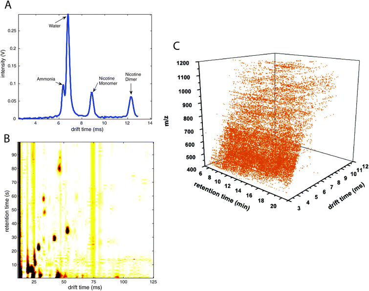 | ||
| Fig. 1 Different data types including ion mobility spectrometry spectra. (A) Ion mobility spectra (1-D data), (B) multicapillary column-ion mobility spectra (2-D data), (C) liquid chromatography-ion mobility-mass spectrometry data (3-D data). (A) is adapted with permission from ref. 19. Copyright (2008) Elsevier. (C) is adapted with permission from ref. 62. Copyright (2006) American Chemical Society. | ||
1.2. Scope of the review
In this paper, we would like to review recent chemometric approaches to analyze ion mobility spectral data coming from analytical systems of different complexities. The general workflow of data analysis is presented in Fig. 2. It is valid not only for analysis of 1-D IMS spectra but also for data analysis of more complex datasets, i.e. 2-D and 3-D IMS datasets. It comprises data preprocessing and pattern recognition steps. A practical example of a full data analysis strategy implemented in the analysis of MCC-IMS spectra is presented in Fig. 3 and discussed further in section 3.3.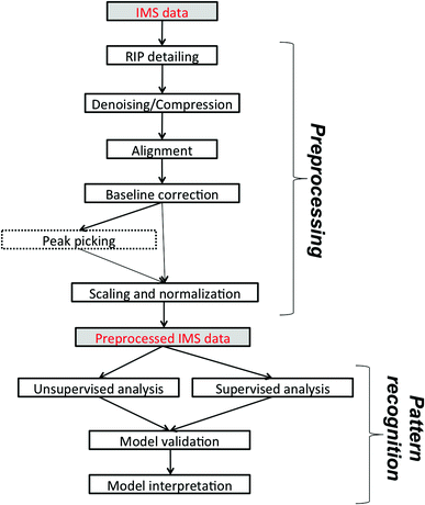 | ||
| Fig. 2 The general workflow of IMS data analysis. Peak picking applies only to targeted analyte analysis. | ||
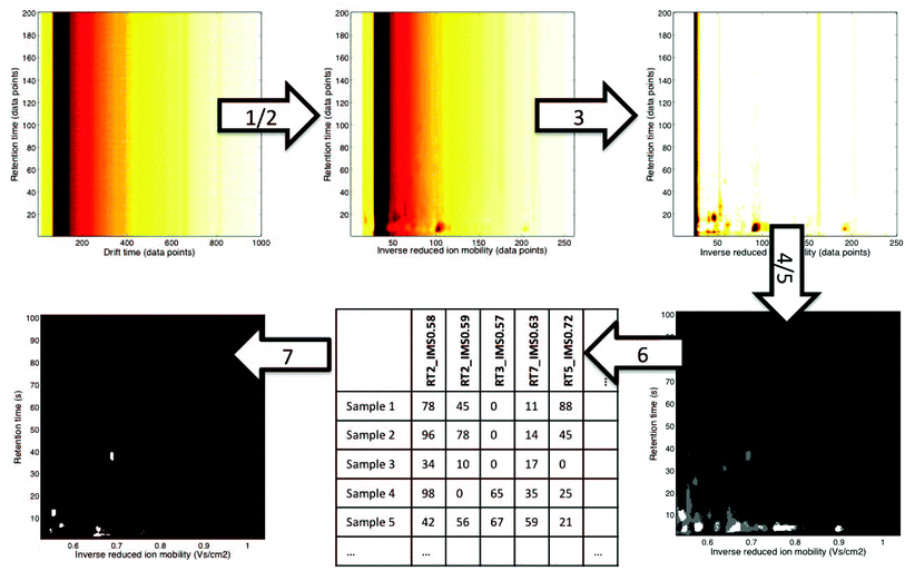 | ||
| Fig. 3 An example of a non-targeted data analysis strategy for MCC-IMS datasets.12 It involves the following steps: (1) alignment: correction of drift times to inverse reduced ion mobility values, (2) denoising in RT dimension and 4× compression in IMS dimension with wavelets, (3) baseline correction with top-hat filtering, (4) region selection: RIP region excluded, (5) mask construction: only white and grey regions are included in the further analysis, (6) data unfolding: levels of variables selected during mask construction are reported for all samples, (7) pattern recognition with sparse-PLS-DA on the data matrix obtained in step 6: a classification model with a number of important variables (white regions are important variables). | ||
Several chemometric techniques and approaches involved in different steps of the data analysis will be discussed and illustrated in this review. Data dimensionality, e.g. 1-D, 2-D or 3-D IMS data, is an important factor in the selection of an appropriate preprocessing technique. In contrast, in pattern recognition, most chemometric techniques can be used for all 1, 2, and 3-D IMS datasets after their previous preprocessing to the proper format. Nevertheless, increasing data size of IMS datasets has to be addressed not only by the development of new preprocessing but also by pattern recognition techniques.
The selection of data analysis techniques depends also on the goal and scope of data analysis. Here, we will focus on two main goals of data analysis: targeted analyte analysis and non-targeted analyte analysis. In targeted analyte analysis, ion mobility data can be used to analyze selected target analytes while ignoring other sample components.11 The identification and quantification of target analytes are the most important steps of targeted analyte analysis. Non-targeted analyte analysis aims at a comprehensive analysis of as many sample components as possible without any prior analyte or component selection.12 Most of the chemometric approaches can be the same in both analysis types. However, their scope and aim are often very different. This is discussed further when specific techniques are introduced.
This paper is organized into the following sections: (2) 1-D IMS data preprocessing, (3) 2-D IMS data preprocessing, (4) 3-D and multi-D IMS data preprocessing, (5) pattern recognition in IMS data analysis, (6) available software and tools, and (7) conclusions and outlook. Sections 2–4 include subsections on targeted analyte analysis and non-targeted analyte analysis. Section 5 comprises subsections on unsupervised and supervised analyses, pattern recognition for large datasets and model validation and interpretation.
2. 1-D IMS data preprocessing
2.1. Data organization
Ion mobility spectra are produced during measurements with an ion mobility spectrometer. They include information about the velocity of gaseous ions in an electric field and the signal intensity, i.e. the amount of ions with the same velocity present in the analyzed sample.Ion velocity is usually expressed as an arrival time or a drift time (ms) or is normalized to standard temperature and pressure as a reduced ion mobility (K0) or an inverse reduced ion mobility (1/K0).13,14 Ion mobility depends on the ion's size, shape, charge and weight (m/z).15 It can also be converted into a collision cross-section (CCS) value, which is a size parameter related to the shape of the molecule, i.e. an averaged momentum transfer impact area of the molecule.16 Several databases include a collection of chemical compounds and their ion mobility. They are either publicly available e.g. for lipids, peptides and proteins10,17,18 or included with commercial software such as the ISAS customized database. The number of ions with the same velocity is usually expressed as the intensity of signals from the Faraday plate of the IMS device in voltage or arbitrary units.
An example IMS spectrum of nicotine is presented in Fig. 1A.19 It comprises peaks of water, ammonia, one monomer and dimer of nicotine. Moreover, the IMS spectra of peanut samples are shown in Fig. 4.20 They contain the reactant ion peak (RIP) and several peaks of compounds present in peanut samples. Ion mobility spectra of different compounds and samples can be used in both qualitative and quantitative analyses.21 Both targeted and non-targeted analyte analysis techniques can be used.
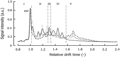 | ||
| Fig. 4 An example of IMS fingerprints of roasted peanuts under different storage conditions. Adapted with permission from ref. 20. Copyright (2016) Elsevier. | ||
2.2. Targeted analyte analysis techniques
IMS instruments have found wide application in the detection of chemical weapons, explosives, environmental pollutants and drugs of abuse. Therefore, the ion mobility of many compounds is known and is used as a reference in their identification. The readout of the standard IMS instrument indices a target analyte peak intensity inside predefined drift time windows selected for each compound. However, the presence of interferences, e.g. other analytes with a similar ion mobility, and changing of peak positions dependent on environmental conditions, e.g. in the field operations, could strongly hamper proper analyte identification and quantification.The post-run data preprocessing and analysis are often being performed to deal with aforementioned problems. This leads to large datasets being stored and analyzed after multiple experiments have been performed e.g. during one hour of monitoring events. Therefore, the main challenge in targeted analyte analysis of IMS data is data preprocessing including feature extraction (i.e. variable selection) and data size reduction (i.e. data compression and variable reduction).22 These are discussed below in sections 2.2.1 and 2.2.2. Proper data preprocessing is usually the most time consuming step of the data analysis pipeline and may shift between success and failure in many applications.23–25
Mixture analysis methods include simple to use interactive self-modelling mixture analysis (SIMPLISMA) and its recursive version (RSIMPLISMA)22,26,27 as well as multivariate curve resolution (MCR) with alternating least squares (ALS).28–31 These methods use multiple IMS spectra collected over time (i.e. different scans) or on different samples.
SIMPLISMA finds pure variables (e.g. the point in the IMS spectrum at which only one analyte is present or which has a constant level of interferences present) and uses the pure variable intensities to estimate the concentration profiles of the target analytes.32 RSIMPLISMA is a speed enhanced modification of SIMPLISMA employing a recursive variance and the Gram–Schmidt distance calculation.22 Multivariate curve resolution with alternating least squares33 is a soft modelling technique based on the assumption that IMS spectra can be modelled as a product of concentration profiles of analytes and a matrix of their spectra. The recently introduced MCR with Least Absolute Shrinkage and Selection Operator (LASSO) allows obtaining automatically the proper number of IMS peaks and their location without a priori knowledge required in the classical MCR.28
Recently, mixture analysis methods were employed in the analysis of IMS spectra of ethanol and benzaldehyde vapors obtained by a luggage scanner,28 chemical weapons in water samples22 and cocaine in urine.30 An example application of mixture analysis methods to IMS spectra is shown in Fig. 5. Here, IMS spectra have been collected over 273 s time for a mixture of two compounds: ethanol and o-nitrotoluene (o-MNT, a taggant for explosive detection) in the presence of interferences (Fig. 5B). Overlaid spectra after baseline correction are shown in Fig. 5A. First estimations for spectra and concentration profiles were obtained by SIMPLISMA (see Fig. 5C and D) and included six components accommodating two main compounds and four interferences. These estimates were included in further analysis with MCR-ALS and MCR-LASSO. Spectra and concentration profiles recovered by MCR-LASSO are shown in Fig. 5E and F. It can be seen that mixture analysis provides full recovery of IMS spectra of analyzed compounds and allows obtaining their concentration profiles in time.
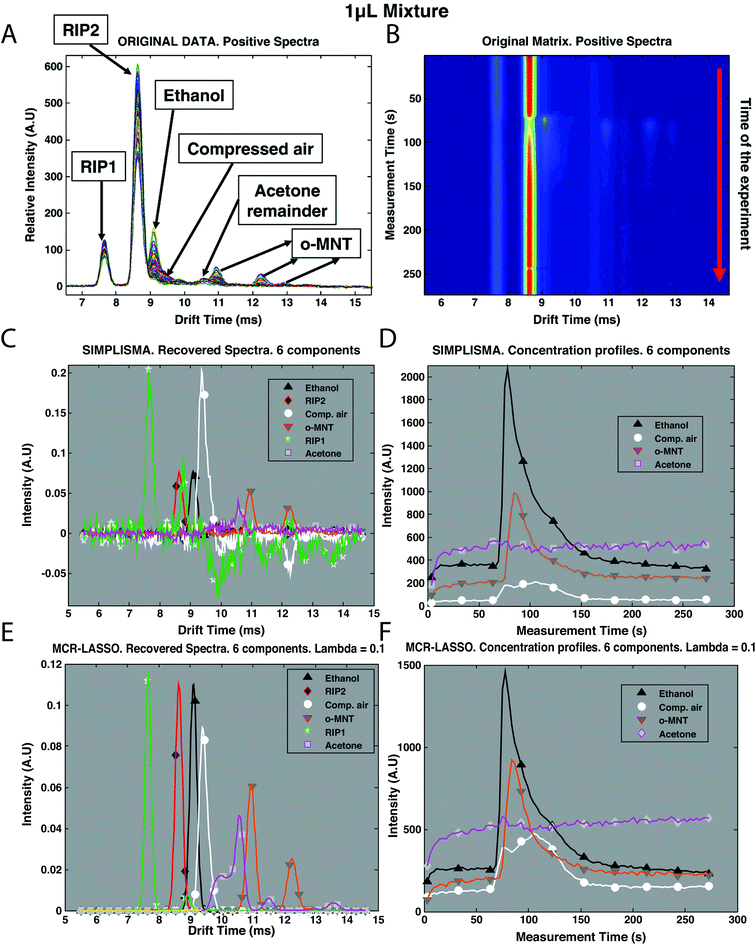 | ||
| Fig. 5 Preprocessing of IMS spectra of the mixture of ethanol and o-MNT in the presence of interferences. (A) Original data after baseline correction, overlaid spectra, intensity vs. drift, (B) original data after baseline correction, time of experiment vs. drift time, (C) original data after baseline correction and SIMPLISMA with 6 components, recovered spectra, (D) original data after baseline correction and SIMPLISMA with 6 components, concentration profiles, (E) original data after baseline correction and MCR-LASSO with SIMPLISMA estimates of 6 components, recovered spectra, and (F) original data after baseline correction and MCR-LASSO with SIMPLISMA estimates of 6 components, concentration profiles. Adapted with permission from ref. 28. Copyright (2010) Elsevier. | ||
Moreover, calibration methods are often implemented in feature extraction steps. These methods include Partial Least Squares (PLS) regression, its modifications such as non-linear PLS,31,34 neural networks (NN)35 and Tucker 3 models.34 They separate overlapping peaks and predict the concentrations of an analyte of interest. Such models are currently in use to analyze the IMS spectra of pesticides34 and drugs such as morphine and noscapine.36
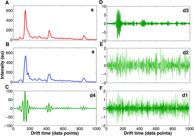
Currently, wavelet transform is the most common compression and denoising method applied to IMS data e.g. in chemical weapons37,39,40 and breath-based disease detection.41,42 Wavelet transform is a mathematical transformation for hierarchically decomposing signals.43 IMS data are particularly suitable for wavelet transformation because of the uniform Gaussian peak shapes that comprise spectra.37 These peaks can be easily distinguished for higher frequency signals such as noise signals. In Fig. 6 an example of IMS spectrum decomposition with wavelet transform is shown. The original spectrum (s, Fig. 6A) is decomposed into one approximation spectrum (a, Fig. 6B) and four detail spectra (d1, d2, d3 and d4, Fig. 6C–F). Denoised IMS spectra can be obtained by reconstruction from the approximation and thresholded detail wavelet coefficients. For example, denoised IMS spectra can be reconstructed from coefficients of the approximation, details d3 and d4, and thresholding coefficients of details d1 and d2, i.e. discarding detail spectra d1 and d2, which could be clearly assumed to be a noise.
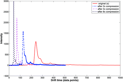
During wavelet compression only selected wavelet coefficients are used. Wavelet compression preserves the relative peak location (i.e. drift time), height and shape. Examples of compressed IMS spectra are displayed in Fig. 7. Here, the original IMS spectrum (in red) is compressed at three levels by selecting wavelet coefficients at different levels. Two, four and eight time compression is obtained by selecting coefficients at the 1st, 2nd or 3rd level.
Different wavelet shapes and levels of compression can be applied to IMS spectra depending on the goal of data analysis, acceptable information loss and the maximum data size allowed. The daublet 8 wavelet filter is one of the most used wavelets for IMS spectra.12,39,42 Strategies including wavelet compression in combination with feature extraction techniques such as SIMPLISMA,38 ALS39 and Partial Least Squares-Discriminant Analysis (PLS-DA)12 allow optimizing wavelet settings and are currently popular.
2.3. Non-targeted analyte analysis techniques
IMS spectra could also be used directly as unique chemical fingerprints of analyzed samples e.g. biological samples, bacterial strains or food products.44–46 An example of IMS fingerprints used for screening the autoxidation of peanuts20 is presented in Fig. 4. IMS fingerprints can be obtained in many different ways, including:(a) single IMS spectrum of a sample of interest,
(b) average IMS spectrum obtained by averaging the intensities at the same drift time across multiple IMS spectra collected for the same sample over time (i.e. different scans or over another separation direction, e.g. over retention time in multicapillary column-ion mobility spectrometry (MCC-IMS)),20,44,47
(c) summary IMS spectrum obtained by summing the intensities at the same drift time across multiple IMS spectra collected for either the same sample over time (i.e. different scans)46 or the same sample at different compensation voltages in the differential mobility spectrometry48 and
(d) unfolding and combining (concatenating) higher dimensional data into 1-D IMS fingerprints e.g. addition of IMS spectra of different glycans (with different m/z values) to an extended drift time axis49,50 or combining IMS spectra at different retention times of MCC-IMS.51
Chemometric analysis of IMS fingerprints comprises several steps including preprocessing and pattern recognition as shown in Fig. 2. Preprocessing usually consists of RIP detailing, denoising, compression, alignment, baseline correction, scaling and normalization. The order of steps may vary depending on data characteristics and the goal of data analysis. Preprocessing methods are listed in Table 2 and described for 1-D IMS data below. Pattern recognition methods are described in section 5.
| Step | Method | 1D | 2D | 3D | Ref. |
|---|---|---|---|---|---|
| RIP detailing | Data cropping | + | + | + | 48 |
| RIP detailing | Curve fitting | + | + | 42 | |
| RIP detailing | Subtraction of baseline | + | + | 54 | |
| Denoising | Wavelets | + | + | + | 12, 37 and 42 |
| Denoising | Savitzky–Golay smoothing | + | + | 47 and 51 | |
| Alignment | Correlation optimized warping (COW) | + | + | 48 | |
| Alignment | Correction by mobility of reactant ion peak | + | 51 | ||
| Alignment | Correction by temperature and pressure (K0) | + | + | 12 and 41 | |
| Alignment | Linear regression | + | 74 | ||
| Baseline correction | Asymmetric least squares (AsLs) | + | 48 | ||
| Baseline correction | Subtraction of baseline without peaks | + | 51 | ||
| Baseline correction | Locally weighted scatterplot smoothing (LOWESS) | + | + | 42 and 55 | |
| Baseline correction | Top-hat filtering | + | 41 | ||
| Scaling | log2 transformation and Pareto scaling | + | 46 | ||
| Scaling | ln![[thin space (1/6-em)]](https://www.rsc.org/images/entities/char_2009.gif) transformation and autoscaling transformation and autoscaling |
+ | 49 | ||
| Scaling | Min–max scaling | + | 48 |
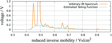 | ||
| Fig. 8 RIP detailing. An IMS spectrum and its estimated tailing function. Adapted with permission from ref. 52. Copyright (2016) Biomed Central. | ||
In most cases data are mean-centered. Scaling to unit variance i.e. autoscaling or range scaling (min–max scaling) is commonly used to obtain similar contributions of each drift time point of IMS fingerprints in the pattern recognition models.48,49 Logarithmic transformation is often implemented to reduce heteroscedasticity observed in IMS spectra.46
IMS spectra can be normalized by the RIP peak intensity, the maximum intensity or internal standard peak intensities. However, in most cases of non-targeted analyte analysis no normalization is performed to solely use IMS spectra as untreated fingerprints.
3. 2-D IMS data preprocessing
3.1. Data organization
Ion mobility spectrometry is often combined either with chromatographic or with mass spectrometric techniques. This means that for each sample a two-dimensional data matrix including IMS dimension and either chromatographic or mass spectrometric dimension is being acquired. An example of the multi capillary column-ion mobility spectrometry (MCC-IMS) data matrix is presented in Fig. 3A. It comprises 200 retention times from MCC and 1000 drift times from IMS modes. This data type is often called an IMS chromatogram. An example of an IMS-MS data matrix is presented in Fig. 9. It contains 500 collision cross-sections from IMS and 2000 mass-to-charge values from MS modes.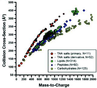 | ||
| Fig. 9 A scatter plot of the CCS values measured in a study described in ref. 60, separated by chemical class. Adapted with permission from ref. 60. Copyright (2014) American Chemical Society. | ||
Including an additional separation dimension with IMS evidently increases information content of the collected data. Nevertheless, both relevant (i.e. compound related) as well as irrelevant and redundant information is provided.12 This leads to a significant increase of the data size and requires more comprehensive data analysis tools for data handling than those for the 1-D IMS data. In many cases, the same chemometric techniques (as those described in section 2) can be used but they are becoming more automated and redesigned to deal with more complex data. These techniques are presented in sections 3.2 and 3.3 for targeted and non-targeted analyte analyses. Specific toolboxes and commercial software including tools presented here are described in section 6.
3.2. Targeted analyte analysis techniques
In the 2-D IMS data, analyte peaks are composed of several points grouped in circle- or oval shaped spots depending on the instrument setup. Thus, in targeted analyte analysis, the preprocessing aim is to identify spots belonging to the target analyte and to quantify its amount in the sample. Therefore peak picking is an important step of targeted analyte data preprocessing. Peak picking of the IMS chromatograms requires different approaches than the 1-D IMS data. These approaches are presented in section 3.2.1.Besides peak picking, preprocessing of IMS chromatograms consists of other steps as presented in Fig. 2, i.e. RIP detailing, denoising, baseline correction, alignment, data scaling and normalization. It leads to the data matrix containing concentrations of target analytes in different samples (i.e. samples × target analyte matrix). Most chemometric techniques used in the preprocessing of IMS chromatograms have already been used in the preprocessing of the single IMS spectra (see the description in section 2). The main differences are related to a chromatographic dimension in the alignment, denoising and baseline correction. Preprocessing techniques common and different for 1 and 2-D IMS datasets are specified in Table 2. Because a majority of preprocessing techniques used for 2-D datasets are common for the targeted and non-targeted analyte analyses, these are discussed in detail in section 3.3.
In contrast, targeted analyte analysis of IMS-MS data focuses on analyte identification. This is because IM is able to separate isobaric analytes based on their dissimilar structural conformation. Structural information in the form of CCS assists in the characterization of analytes by biomolecular class, as these classes are known to separate in IM-MS space60 (see Fig. 9). Different regression curves can be fitted per class of compounds and power-law relationships seem to describe the correlations between CCS and m/z values the best.60 These relationships partition the IM-MS space into distinct bands which can be subjected to a probability distribution analysis for molecular class information, acting as so called biomolecular filtering.61,62
Chemometric techniques are involved in defining aforementioned relationships e.g. separate relationships for different lipid classes can be obtained by linear regression63 as well as by deriving probability distributions reflecting structure variability within a class. On another level, the CCS of a specific compound can be predicted based on its m/z value, class belongingness and other intrinsic size parameters.64 Chemometric techniques such as Partial Least Squares regression (PLSR) and Support Vector regression (SVR) are commonly employed in this process.
So far, there have been limited references to chemometric techniques specifically adapted for IMS-MS data preprocessing and analysis. Amphirite is a software package for automated extraction of drift times of ions coming from the same compound and their transformation to CCS.65 Most of the techniques described for 1-D IMS data (see section 2) are successfully implemented to IMS-MS data after data unfolding or selection of IMS spectra with a specific m/z value.49,50,66
The merged peak cluster localization is present in the commercial software package Visual Now (B&S Analytik, Dortmund, Germany). MPCL is based on a procedure introduced by Bader et al.,69 in which points of the IMS chromatogram are firstly clustered with k-means clustering with Euclidean distance and then merged following a concept for image segmentation.70 The watershed transformation method is adapted from the spot detection on 2D gel electrophoresis images. WST is described for IMS data by Bunkowski54 and included in the IPHEx software. The IMS chromatogram is treated as a landscape including hills and valleys and algorithm is filling the turned upside-down landscape with water, annotating which points of the IMS chromatograms show similar behavior. D'Addario et al. use a peak model estimation algorithm in a modular framework for automated peak detection PEAX.71 Here, each peak is described by a model function consisting of two shifted inverse Gaussian distributions and an additional peak volume parameter. D'Addario reported that her approach yielded 74% agreement with manual peak annotation. Hauschild et al.72 discovered that the manual peak annotation by domain experts yields the best results for sample classification when it is compared to automatic peak picking techniques and software (e.g. IPHEx54 or Visual Now69). Thus it is reasonable to optimize peak picking algorithms towards a domain expert. It is sensible to mention that manual peak picking often takes hours while automated peak picking is ready in only a few seconds.
3.3. Non-targeted analysis techniques
Non-targeted analyte analysis for the 2-D IMS data aims at broadening the scope of targeted analyte analysis above a priori picked peaks and spectral regions. The first non-targeted data analysis strategy for MCC-IMS datasets was recently introduced by Szymańska et al.12 It is presented in Fig. 3. It includes several chemometric techniques used in preprocessing i.e. alignment, denoising, compression, baseline correction, region selection and a discriminant analysis. Importantly, data size reduction steps are implemented into this strategy enabling effective classification of different samples and the selection of spectral regions important for their classification. Data size reduction is achieved in three complementary steps: by compression with wavelet transform (step 2), by mask construction (step 5) and by variable selection during discriminant analysis with sparse-partial least squares-discriminant analysis (s-PLS-DA) (step 7). This ultimately leads to a reduction in data size up to 50 variables relevant to the goal of analysis and a great improvement in sample classification results. Therefore, this strategy is a novel alternative and complements targeted approaches.Several chemometric techniques are currently being modified or adapted for 2-D IMS data. They are mainly based on techniques employed in the comprehensive analysis of either the 2D chromatographic data, such as the GC × GC data, LC × LC data and 2D-electrophoresis,11 or in the image analysis.41,73 Some examples of these techniques are presented below.
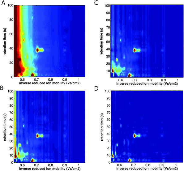 | ||
| Fig. 10 Baseline correction of MCC-IMS spectra of a single exhaled breath sample. (A) Before baseline correction, (B) after baseline correction with minimum subtraction, (C) after baseline correction with first line subtraction, and (D) after baseline correction with top-hat method. The color scale is fixed across all images. Adapted with permission from ref. 41. Copyright (2016) Elsevier. | ||
4. 3-D and multi-D IMS data preprocessing
Combination of IMS with both chromatography and mass spectrometry can lead to 3-D and multidimensional datasets.5 Very recently, such multidimensional datasets were produced and analyzed in many omics studies including metabolomics, proteomics, lipidomics and glycomics studies.5,9,10,62,77,78High-dimensional datasets place particular demands on the chemometrics used to infer desired information from these system-wide data. During data preprocessing it is complicated to extract peak features correlated across such data. The powerful software available for UHPLC-MS and GC-MS data (as well as GC-GC-MS etc.) are not equipped to account for the ion mobility dimension while compiling the data matrix for the multivariate analysis. Therefore, the complexity of the data is often reduced in the initial stages of the analysis by collapsing the IMS dimension.78
Nevertheless, new automated preprocessing strategies (e.g. the LC-IMS-MS finder) were recently developed to include IMS dimension, especially focusing on distinct IMS drift times for multiple charges states of the same compounds.79,80 The LC-IMS-MS finder is especially useful when: (1) a single compound exists in multiple structural conformations that have distinct IMS drift times and (2) two different compounds co-elute in IMS dimension.79 A number of extracted peaks are dependent on the complexity of the sample, experimental conditions of the LC-IMS-MS method and the tool used in the peak extraction. More than 4000 peaks can be extracted from the LC-IMS-MS dataset on saliva samples78 and sera samples.77 Tebani et al. used a number of extracted peaks and a number of reliable peaks as a response variable in experimental design in the optimization of the LC-IMS-MS method.77 It is expected that more and more applications of chemometric techniques in the analysis of such data will come in the near future, when novel LC-IMS-MS and GC-IMS-MS instruments will become more popular.
5. Pattern recognition techniques
Selection of a pattern recognition technique is determined by the goal of data analysis, by data characteristics and by chemometric technique's popularity in the given application field. The goal of data analysis can be either qualitative or quantitative.21 Qualitative goal relates to sample classification, discrimination and biomarker detection. Quantitative goal mainly focuses on calibration problems. Data characteristics refer to the data dimensionality, its information content and the applied preprocessing procedure. The application field, e.g. process analytical technology, clinical metabolomics, or breath research, often imposes which techniques are recommended and commonly used.Both univariate and multivariate statistical techniques can be used. Univariate techniques e.g. analysis of variance (ANOVA) focuses on one variable at a time e.g. one spectral variable with a specific ion mobility. Multivariate techniques analyze all variables simultaneously e.g. IMS spectra composed of hundreds or thousands of variables are evaluated at once. Thus multivariate techniques utilize the information on variable correlations that has been proven to be beneficial for obtaining statistical models with higher sensitivity and specificity.81 This phenomenon is often referred to as a multivariate advantage.
Pattern recognition often starts with the data visualization and exploratory analysis. Unsupervised chemometric techniques are often used in this step, giving a first and unbiased view on data. Next, supervised techniques are used utilizing a priori knowledge on the data e.g. sample classes. Finally, pattern recognition results are statistically validated and the goal-driven interpretation is provided. Chemometric techniques used in the pattern recognition of IMS data are shortly described below. For a more extensive description of pattern recognition techniques we refer the reader to several chemometric books and articles.21,67,82 Finally, we list the applications of these techniques to IMS data in Table 3.
| Step | Method | Ref. |
|---|---|---|
| Unsupervised analysis | Principal Component Analysis (PCA) | 44, 46–48, 50 and 51 |
| Unsupervised analysis | Cluster analysis (HCA) | 20, 84 and 87 |
| Unsupervised analysis | Multidimensional Scaling (MDS) | 87 |
| Unsupervised analysis | Self-organizing maps (SOM) | 86 |
| Supervised analysis | Partial least squares-discriminant analysis (PLS-DA) | 48 |
| Supervised analysis | Sparse-PLS-DA | 12 and 41 |
| Supervised analysis | Linear discriminant analysis (LDA) | 44, 47 and 51 |
| Supervised analysis | Recursive support vector machine (r-SVM) | 46 and 88 |
| Supervised analysis | Random forests (RF) | 46 and 88 |
| Supervised analysis | Genetic algorithms (GA) | 50 |
| Supervised analysis | k-Nearest neighbor (k-NN) | 47 and 51 |
| Supervised analysis | Principal component regression (PCR) | 97 |
| Supervised analysis | Partial least squares regression (PLSR) | 94, 97 and 98 |
| Supervised analysis | n-Way partial least squares regression (n-PLSR) | 36 and 95 |
5.1. Unsupervised analysis
Chemometric techniques used in the exploratory analysis consist of two types of techniques: projection techniques (e.g., principal component analysis (PCA)) and partitional clustering techniques (e.g., hierarchical cluster analysis (HCA)).Principal component analysis is the most widely used explorative analysis technique. It summarizes data into a small number of linearly uncorrelated principal components (PCs), representing samples in a matrix of scores and variables in a matrix of loadings. PCA results are usually presented as a score plot and a loading plot. In the score plot (see Fig. 11A, ref. 83), a single point represents a sample (here, an olive oil sample) and the proximity of this point to other points can be interpreted as the similarity of this sample (here, in its IMS spectrum) to other samples. Grouping of olive samples per olive oil type can be seen but sample groups partially overlap (see triangles, asterisks and squares). In the loading plot (not shown), a single point (or an arrow) represents a variable (e.g. a data point of IMS spectra, an IMS peak). Its location refers to its contribution to the distribution of samples in the score plot. Additionally, the correlation between variables is reflected by the angle between arrows in the loading plot.
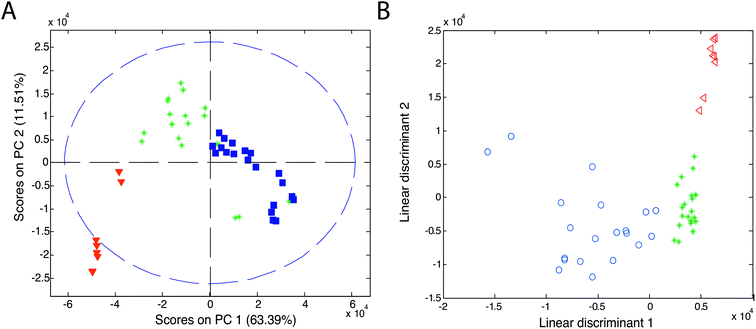 | ||
| Fig. 11 Score plots of (A) PCA and (B) LDA analyses of olive oils. Blue symbols refer to virgin olive oil, green asterisks refer to olive oil and red triangles refer to pomace olive oil. Adapted with permission from ref. 83. Copyright (2011) Elsevier. | ||
PCA analysis is well suited for the visualization of high-dimensional datasets as well as for the data size reduction. It is because the data are represented in a limited number of PCs. It is especially useful when dominant sources of variation are known and are of interest for the analyzed dataset. Recent PCA applications include food authentication,47,83,84 bacterial strains identification,48 flavor analysis,85 disease diagnosis49,50 and many others.
Self-Organizing Maps (SOMs) are another class of projection techniques used for the IMS data. They construct a non-linear projection of the data onto a low-dimensional display, which can also be used to observe a possible clustering.21 SOMs are used to prioritize features from the LC-IMS-MS data of bacterial cocultures86 and integrate different sources of data within one analysis e.g. IMS-MS data and transcriptomics data.10 SOMs for 4 bacterial cocultures and 5 monocultures (Nocardiopsis and 4 challenger organisms) are constructed and presented as heatmaps in Fig. 12.86 In this case, SOMs organized metabolomic features (from UPLC/IMS-MS measurements) into single tiles such that features with similar profiles (e.g. temporal intensity profiles, response to experimental conditions, etc.) are localized in the same or adjacent space. The results of SOMs are visually interpretable heatmaps in which features are localized according to their profiles and tiles are colored by the centroid integrated intensity of features they contain. The difference of the coculture SOM from the monoculture SOM results in a coculture response map highlighting unique and upregulated features.
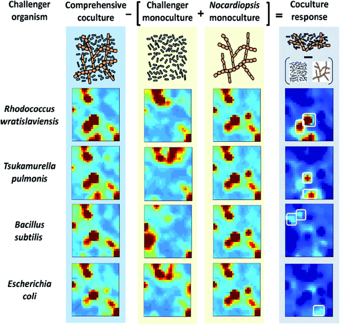 | ||
| Fig. 12 Self-organizing map (SOM) analysis of UPLC/IM-MS datasets on mono- and cocultures. Heatmaps of features of 4 cocultures and 5 monocultures (Nocardiopsis and 4 challenger organisms) are presented. The difference of the coculture SOM from the monocultures results in a coculture response heatmap highlighting only those features that are distinct from the monocultures. Adapted with permission from ref. 86. Copyright (2014) American Chemical Society. | ||
Partitional clustering techniques are commonly applied when the goal of data analysis is to group samples based on their IMS spectra or IMS peak profile. Clustering techniques use different similarity measures (e.g. Euclidean distance, Manhattan distance or 1 − correlation) to partition the dataset into sample clusters. HCA uses distances to assess which samples are similar and then organizes them into an ordered grouping, referred to as a hierarchical tree or dendrogram. Depending on the set of thresholds, the result of one clustering algorithm is a list of groupings, each corresponding to a certain threshold. An example dendrogram of IMS spectra of peanut samples stored under different conditions is shown in Fig. 13. Here, HCA with Euclidian distance and average linkage method lead to different groups of peanuts depending on the time (0, 14, and 21 days’ storage) and type of their storage (open or sealed). The selected threshold is indicated by a vertical line.
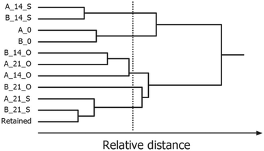 | ||
| Fig. 13 Hierarchical cluster analysis of IMS spectra of roasted peanuts. A dendrogram was obtained for two peanut lots: A and B, 0, 14, 21 days of storage, O, S, open or sealed storage. Adapted with permission from ref. 20. Copyright (2016) Elsevier. | ||
HCA and similar methods such as transitivity clustering87 work very well when a hierarchical structure is present in the data. Hauschild et al.87 propose a breathomics clustering workflow including data clustering, visualization with multidimensional scaling (MDS), assessment of clustering quality and selection of sample and variable subsets. In this workflow breath samples coming from different patient groups can be clustered and the effect of other factors such as age, gender on clustering can be observed. Partitional clustering techniques were also recently applied to IMS data in food shelf-life monitoring20 and adulteration detection.84
Alternatively, k-means clustering also uses a proximity measure, but partitions the dataset into a pre-defined number of clusters. The user has to define a number of clusters. k-means clustering selects a set of centroids, which correspond to a number of clusters, in such a manner that the summary distance of all samples to the centroids is minimized. So far, this technique has been applied mainly in peak clustering of MCC-IMS data (see section 3.2.1).70
5.2. Supervised analysis
Supervised analysis techniques use a priori knowledge about the obtained data, either sample classes: treatment groups and groups of patients or specific sample properties e.g. specific compound content. They employ this knowledge to evaluate:(a) whether the data contain any patterns related to them,
(b) how strong these patterns are, and
(c) whether they can be used to predict the knowledge for new samples.
The main goal of supervised techniques is to find the relationship between a matrix of predictors (data matrix X, here: IMS spectral variables in different samples or IMS peaks in different samples) and a vector (or a matrix) of responses (Y vector, e.g. the class membership and concentration of a specific compound). This relationship can be linear or non-linear; this determines which chemometric technique will be most suited to investigate it. Linear discriminant analysis (LDA), partial-least squares-discriminant analysis (PLS-DA), k-nearest neighbor (k-NN), neural networks (NN), support vector machine (SVM), random forests (RF), and genetic algorithms (GP) are commonly employed in the classification of IMS data.12,41,47,69,83,84,88 The performances of several chemometric techniques were evaluated and compared for a single MCC-IMS dataset on the chronic obstructive pulmonary disease by Hauschild et al.88
Linear discriminant analysis is the most popular classification technique for the IMS data.51,55,69,83,89,90 LDA can be performed directly on the dataset or after PCA analysis on a selected number of principal components (PCA-LDA approach). An example of the classification results of linear discriminant analysis is presented in Fig. 11B. Here, a clear classification of olive samples into extra virgin olive oil, olive oil and pomace olive oil classes was obtained with the PCA-LDA approach.83 For this dataset, 100% classification was also obtained with the k-NN classifier with three nearest neighbors. Three distinct groups are visible in the PCA-LDA plot contrary to the PCA score plot in Fig. 11A. This clearly demonstrates the main difference between the unsupervised and supervised approaches. PCA-LDA solely focuses on finding differences between sample classes (supervised approach), while PCA analysis is an exploratory approach in which clear group separation may or not be the outcome of the analysis (depending on the dominant sources of variation in the data).
PLS-DA is commonly employed in metabolomics studies on disease diagnosis and in food screening, and also with IMS data.41,48,67,91,92 PLS performs dimensionality reduction to latent variables (LVs, similar to PCs in PCA). Latent variables are obtained by maximizing the covariance between a data matrix X and a dummy class vector Ye.g. class membership. PLS-DA can deal with highly collinear data; this can be especially useful for the IMS fingerprint data. Several modifications and improvements of the PLS-DA technique exist, including sparse-PLS-DA, recently introduced in the IMS data analysis by Szymańska et al.12 A sparse version of PLS-DA aims at combining variable selection and classification into a one-step procedure.93 In the case of highly redundant data such as IMS data, this technique has been proven to give superior results compared to the standard PLS-DA analysis using all variables.
Regression techniques including multivariate linear regression, principal component regression (PCR), partial least squares regression (PLSR) and n-way PLSR (n-PLSR) are also frequently employed in the analysis of the IMS data94 (see Table 3). They are routinely used in food quality and safety control analyses,94,95 environmental analyses96–98 and in process monitoring.99 Detailed information about these chemometric techniques can be found in ref. 82, 100 and 101.
5.3. Pattern recognition techniques for large datasets
The large data size, its megavariate nature (more than a million variables per sample) as well as the redundancy of information (several variables (pixels) associated with one compound) in 2-D and more-D IMS data may significantly hamper pattern recognition, especially in non-targeted analyte analysis. It is because of computational challenges e.g. “out of memory” problems and extensively long computation times occurring when data are exported from the analytical equipment and analyzed on the standard PC. It is also because of a lack of suitable chemometric techniques. Most pattern recognition techniques, described in sections 5.2 and 5.3, cannot handle properly megavariate data sets, leading to overfitting and false positive associations.21The common solutions are reducing the data size and developing novel chemometric techniques, especially for large datasets. Data size reduction can be obtained by data compression not only during data preprocessing but also during pattern recognition. This can be achieved to some extent by either variable reduction e.g. PCA or PLS or by variable selection e.g. mask construction and variable selection included in discriminant analysis. A combination of different techniques and approaches is advisable because it leads to the increase of model performance. This was shown by Szymańska et al.,12 mentioned in section 3.3 and presented in Fig. 3.
While variable reduction is implemented, many correlated variables (i.e. redundant variables) are transformed into one latent variable. On the other hand, during variable selection only variables important for the goal of data analysis are selected. Depending on the variable selection technique and the selection criteria, it can happen that only one out of many correlated variables is included in the selection. The rest is discarded.
Mask construction, one of variable selection techniques, selects variables based on predefined criteria, related to both data characteristics and the goal of data analysis. It was recently adapted from image analysis.12,41,73 In Fig. 14, masks constructed for the MCC-IMS dataset41 with two classes of samples: healthy controls and asthma are shown. They were constructed per class eliminating variable with intensities lower than the set limit of detection (LOD) in more than 90% of the samples. It can be seen that selected variables (white spots) include numerous peaks (spots). Each peak is described by many correlated variables that can further help in the interpretation.73 Common and different variables between two sample classes can be clearly seen and evaluated.
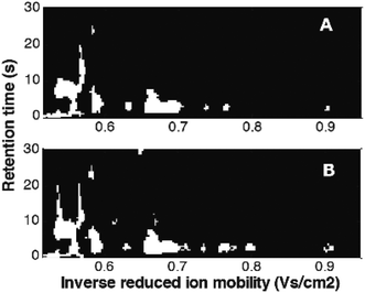 | ||
| Fig. 14 Masks constructed for the breathomics dataset:41 (A) mask for healthy controls and (B) mask for asthma patients. Adapted with permission from ref. 41. Copyright (2016) Elsevier. | ||
There are many variable selection techniques combined with supervised pattern recognition tools.12,41,46,88 Sparse-PLS-DA is one of the recently used techniques.12 By simultaneous variable reduction (PLS) and variable selection by sparsity constraints, correlated variables from the same MCC-IMS peak, which are important for classification, are selected. This improves both model interpretation (ca. 100 variables, belonging to 5–6 peaks12) and model performance. In the recursive SVM (r-SVM) classification, models were recursively built using different variable subsets. The model with the minimum number of variables and minimum cross-validation error is selected as the final model.46 In the case of detection of adulteration of sesame oil, all 650 variables from IMS fingerprints are used to obtain an accuracy of 94%.46 In the study by Hauschild et al. on COPD classification, it was shown that subsets of variables selected by different classifiers do not always overlap.88 This is due to the different underlying approaches, in some cases linear models (e.g. linear SVM) and in the other cases non-linear models (e.g. random forests).
5.4. Model validation and interpretation
Pattern recognition techniques are usually combined with proper validation procedures including internal and external validation. During internal validation the parameters of a technique are optimized e.g. the number of latent variables and the number of selected variables. External validation focuses on the generalization of obtained models to new samples. Thanks to model validation a certainty can be given to model findings e.g. the relationship between IMS spectra and the presence of lung cancer. Moreover, different chemometric models and procedures obtained on the same dataset can be further evaluated and compared.51The most common validation approaches include resampling methods such as leave-one-out cross-validation, double cross-validation, bootstrapping and permutation tests.12,41,46,47,55 The choice of the resampling procedure is mainly determined by the number of samples available in a dataset. In the ideal case, the dataset is divided into a training set (used to train the classification or calibration model), a validation set (employed to optimize the model parameters (internal validation)) and an independent test set employed to assess the predictive power of the model (external validation). Currently, due to the increase in computer power and speed, extended resampling approaches (e.g. double cross-validation combined with permutation tests) are increasingly used, even for complex high-dimensional data.
Performance parameters assessed during internal and external validation relate to the presence of errors in the results (samples assigned to the wrong classes and differences between predicted and true values in the calibration models). There are many performance parameters including and not limited to a number of misclassifications, accuracy, sensitivity, specificity, area under ROC curve (AUROC) and root mean square error of prediction (RMSEP). The detailed information about these performance parameters is provided in ref. 21, 102 and 103.
Model interpretation is usually the last step of data analysis workflows, where the relevance of model findings is assessed for the context and application area of the study. This refers to the interpretation of variables selected by a chemometric model as significant for classification or calibration. Selected variables may refer to disease biomarkers,104 bacterial identification compounds,105 food biomarkers51etc.
6. Software
Several chemometric techniques applicable to the IMS data are already available as toolboxes and software packages. Some of them have already been described in sections 2–5. Additionally, we have listed and described them in Table 4. They include both different preprocessing as well as pattern recognition tools. Other software packages developed for metabolomics and proteomics data analysis can be also used for the IMS data, but these are not referenced here.| Name | Goal | Availability | Ref. |
|---|---|---|---|
| Excellims VisIon | Data visualization, peak finding and referencing of IMS data | Commercial software from Excellims, http://www.excellims.com/products/vision-software/ | 108 |
| Visual Now | Data visualization, peak finding and referencing of MCC-IMS data | Commercial software from B&S Analytik, http://www.bs-analytik.de/eprodukte.html | 109 |
| IMMS extension to Drifscope | Preprocessing of IMS spectra onto data formats enabling peptide identification and referencing | Open access, http://code.google.com/p/ion-mobility-ms-tools.html | 110 |
| Amphitrite | Extraction of IMS profiles of single compounds | Open access, http://www.homepages.ucl.ac.uk/~ucbtkth/amphitrite.html | 65 |
| EM-IM | Relating IMS data with electron microscopy data | Open access, http://EMnIM.chem.ox.ac.uk.html | 111 |
| MIMA | Automated identification of MCC-IMS peaks by referencing with GC-MS data | Open access, http://mima.mpi-inf.mpg.de | 112 |
| LC-IMS-MS feature finder | Detection of multidimensional LC-IMS-MS feature | Open access, http://omics.pnl.gov/software/LC-IMS-MS_Feature_Finder.php | 79 |
| Carotta | Unsupervised pattern recognition of MCC-IMS data | Open access, http://carotta.compbio.sdu.dk | 87 |
7. Conclusions and outlook
The present paper provides a complete overview of different types of ion mobility spectrometry data as well as the main chemometric techniques involved in their analysis. Recent advancements in ion mobility spectrometry instruments, especially coupling with different separation techniques, led to multidimensional IMS datasets. These have to be combined with sophisticated chemometric techniques in order to benefit from a plethora of information they bring. In this paper, we show recent examples of available chemometric techniques employed in IMS data analysis. These include different preprocessing and pattern recognition tools, nowadays often combined into automated or semi-automated data analysis strategies. The presented examples clearly demonstrate the significant contribution of chemometric tools to the recent and great expansion of ion mobility spectrometry technology into different application fields.From reviewing the work in this field, there is one area which needs addressing, and the field is mature enough for the community to re-address this with some focus. The innovative work described above tends to be limited to addressing individual problem areas on individual researchers’ experimental setups, whether applying commercial instrumentation or outside of the research prototype stage. If the field is to advance at the pace that it is clearly capable of doing, there needs to be renewed effort by thought leaders in the field to solve the issues around transferability of the analyses and derived chemometric models between instruments of different manufacturers. The issues with the data described in this review are not far removed from those faced by the near infrared (NIR) spectroscopy community in the past.106,107 Similarities to the NIR also exist in the potential to deploy cheaper, robust ion mobility instrumentation into the wider world exploiting the results and models generated by high-end research-grade systems.
We conclude that well-thought out, comprehensive data analysis strategies including several chemometric techniques should and will be applied to IMS datasets in the future. These strategies should address two main issues: (a) data complexity and dimensionality i.e. by data size reduction and (b) a comprehensive and automated compound identification i.e. by combining information from available separation dimensions such as chromatography, ion mobility spectrometry and mass spectrometry. There is no doubt that obtaining and implementing comprehensive data analysis strategies is an essential milestone for the next decade of IMS technology advancements.
Acknowledgements
This research received funding from the Netherlands Organization for Scientific Research (NWO) in the framework of the Technology Area COAST, project 053.21.109. Ewa Szymańska would like to thank Sanne van den Dikkenberg for her assistance in the literature search.References
- R. Cumeras, E. Figueras, C. Davis, J. Baumbach and I. Gràcia, Analyst, 2015, 140, 1391–1410 RSC.
- C. D. Chouinard, M. S. Wei, C. R. Beekman, R. H. Kemperman and R. A. Yost, Clin. Chem., 2016, 62, 124–133 Search PubMed.
- J. C. May and J. A. McLean, Anal. Chem., 2015, 87, 1422–1436 CrossRef CAS PubMed.
- M. T. Bowers, Int. J. Mass Spectrom., 2014, 370, 75–95 CrossRef CAS PubMed.
- S. J. Valentine, X. Liu, M. D. Plasencia, A. E. Hilderbrand, R. T. Kurulugama, S. L. Koeniger and D. E. Clemmer, Expert Rev. Proteomics, 2005, 2, 553–565 CrossRef CAS PubMed.
- C. S. Hoaglund, S. J. Valentine, C. R. Sporleder, J. P. Reilly and D. E. Clemmer, Anal. Chem., 1998, 70, 2236–2242 CrossRef CAS PubMed.
- Waters, http://www.waters.com, assessed on 15.2.2016.
- Agilent, http://www.agilent.com, assessed on 15.2.2016.
- M. Holčapek, R. Jirásko and M. Lísa, J. Chromatogr., A, 2012, 1259, 3–15 CrossRef PubMed.
- S. D. Sherrod and J. A. McLean, Clin. Chem., 2016, 62, 77–83 CAS.
- K. M. Pierce, B. Kehimkar, L. C. Marney, J. C. Hoggard and R. E. Synovec, J. Chromatogr., A, 2012, 1255, 3–11 CrossRef CAS PubMed.
- E. Szymańska, E. Brodrick, M. Williams, A. N. Davies, H.-J. van Manen and L. M. C. Buydens, Anal. Chem., 2015, 87, 869–875 CrossRef PubMed.
- W. Vautz, B. Bödeker, J. I. Baumbach, S. Bader, M. Westhoff and T. Perl, Int. J. Ion Mobility Spectrom., 2009, 12, 47–57 CrossRef CAS.
- C. J. Denawaka, I. A. Fowlis and J. R. Dean, J. Chromatogr., A, 2014, 1338, 136–148 CrossRef CAS PubMed.
- G. A. Eiceman, Z. Karpas and H. H. Hill Jr., Ion mobility spectrometry, CRC Press, 2013 Search PubMed.
- E. W. McDaniel and E. A. Mason, Mobility and diffusion of ions in gases, John Wiley and Sons, New York, 1973 Search PubMed.
- S. C. Henderson, S. J. Valentine, A. E. Counterman and D. E. Clemmer, Anal. Chem., 1999, 71, 291–301 CrossRef CAS PubMed.
- M. F. Bush, Z. Hall, K. Giles, J. Hoyes, C. V. Robinson and B. T. Ruotolo, Anal. Chem., 2010, 82, 9557–9565 CrossRef CAS PubMed.
- R. M. O'Donnell, X. Sun and P. d. B. Harrington, TrAC, Trends Anal. Chem., 2008, 27, 44–53 CrossRef.
- M. Tzschoppe, H. Haase, M. Höhnisch, D. Jaros and H. Rohm, Food Control, 2016, 64, 17–21 CrossRef CAS.
- E. Szymańska, J. Gerretzen, J. Engel, B. Geurts, L. Blanchet and L. M. Buydens, TrAC, Trends Anal. Chem., 2015, 69, 34–51 CrossRef.
- P. J. Rauch, P. d. B. Harrington and D. M. Davis, Chemom. Intell. Lab. Syst., 1997, 39, 175–185 CrossRef CAS.
- J. Engel, J. Gerretzen, E. Szymańska, J. J. Jansen, G. Downey, L. Blanchet and L. M. Buydens, TrAC, Trends Anal. Chem., 2013, 50, 96–106 CrossRef CAS.
- E. Szymańska, M. Markuszewski, X. Capron, A.-M. Van Nederkassel, Y. Vander Heyden, M. Markuszewski, K. Krajka and R. Kaliszan, J. Pharm. Biomed. Anal., 2007, 43, 413–420 CrossRef PubMed.
- J. Gerretzen, E. Szymańska, J. J. Jansen, J. Bart, H.-J. van Manen, E. R. van den Heuvel and L. M. Buydens, Anal. Chem., 2015, 87, 12096–12103 CrossRef CAS PubMed.
- G. Chen and P. de B Harrington, Anal. Chim. Acta, 2003, 484, 75–91 CrossRef CAS.
- M. L. Ochoa and P. B. Harrington, Anal. Chem., 2004, 76, 985–991 CrossRef CAS PubMed.
- V. Pomareda, D. Calvo, A. Pardo and S. Marco, Chemom. Intell. Lab. Syst., 2010, 104, 318–332 CrossRef CAS.
- T. L. Buxton and P. d. B. Harrington, Anal. Chim. Acta, 2001, 434, 269–282 CrossRef CAS.
- Y. Lu, R. M. O'Donnell and P. B. Harrington, Forensic Sci. Int., 2009, 189, 54–59 CrossRef CAS PubMed.
- V. Pomareda, A. V. Guamán, M. Mohammadnejad, D. Calvo, A. Pardo and S. Marco, Chemom. Intell. Lab. Syst., 2012, 118, 219–229 CrossRef CAS.
- E. Szymańska, M. J. Markuszewski, Y. Vander Heyden and R. Kaliszan, Electrophoresis, 2009, 30, 3573–3581 CrossRef PubMed.
- A. de Juan and R. Tauler, Crit. Rev. Anal. Chem., 2006, 36, 163–176 CrossRef CAS.
- T. Khayamian, S. Sajjadi, S. Mirmahdieh, A. Mardihallaj and Z. Hashemian, Chemom. Intell. Lab. Syst., 2012, 118, 88–96 CrossRef CAS.
- P. Zheng, P. d. B. Harrington and D. M. Davis, Chemom. Intell. Lab. Syst., 1996, 33, 121–132 CrossRef CAS.
- T. Khayamian, M. Tabrizchi and M. Jafari, Talanta, 2006, 69, 795–799 CrossRef CAS PubMed.
- A. A. Urbas and P. B. Harrington, Anal. Chim. Acta, 2001, 446, 391–410 CrossRef.
- G. Chen and P. B. Harrington, Anal. Chim. Acta, 2003, 490, 59–69 CrossRef CAS.
- L. Cao, P. d. B. Harrington and C. Liu, Anal. Chem., 2004, 76, 2859–2868 CrossRef CAS PubMed.
- L. Cao, P. d. B. Harrington, C. S. Harden, V. M. McHugh and M. A. Thomas, Anal. Chem., 2004, 76, 1069–1077 CrossRef CAS PubMed.
- E. Szymańska, G. H. Tinnevelt, E. Brodrick, M. Williams, A. N. Davies, H.-J. van Manen and L. M. Buydens, J. Pharm. Biomed. Anal., 2016, 127, 170–175 CrossRef PubMed.
- S. Bader, W. Urfer and J. I. Baumbach, Int. J. Ion Mobility Spectrom., 2008, 11, 43–49 CrossRef CAS.
- F. Ehrentreich, Anal. Bioanal. Chem., 2002, 372, 115–121 CrossRef CAS PubMed.
- R. Alonso, V. Rodríguez-Estévez, A. Domínguez-Vidal, M. J. Ayora-Cañada, L. Arce and M. Valcárcel, Talanta, 2008, 76, 591–596 CrossRef CAS PubMed.
- R. Vinopal, J. Jadamec, A. Demars, S. Jakubielski, C. Green, C. Anderson, J. Dugas and R. DeBono, Anal. Chim. Acta, 2002, 457, 83–95 CrossRef CAS.
- L. Zhang, Q. Shuai, P. Li, Q. Zhang, F. Ma, W. Zhang and X. Ding, Food Chem., 2016, 192, 60–66 CrossRef CAS PubMed.
- R. Garrido-Delgado, L. Arce, A. Guamán, A. Pardo, S. Marco and M. Valcárcel, Talanta, 2011, 84, 471–479 CrossRef CAS PubMed.
- W. Cheung, Y. Xu, C. P. Thomas and R. Goodacre, Analyst, 2009, 134, 557–563 RSC.
- D. Isailovic, M. D. Plasencia, M. M. Gaye, S. T. Stokes, R. T. Kurulugama, V. Pungpapong, M. Zhang, Z. Kyselova, R. Goldman and Y. Mechref, J. Proteome Res., 2011, 11, 576–585 CrossRef PubMed.
- M. Gaye, S. Valentine, Y. Hu, N. Mirjankar, Z. Hammoud, Y. Mechref, B. Lavine and D. Clemmer, J. Proteome Res., 2012, 11, 6102–6110 CAS.
- R. Garrido-Delgado, L. Arce and M. Valcárcel, Anal. Bioanal. Chem., 2012, 402, 489–498 CrossRef CAS PubMed.
- D. Kopczynski and S. Rahmann, Algorithms Mol. Biol., 2015, 10, 1–14 CrossRef CAS PubMed.
- D. Kopczynski, J. I. Baumbach and S. Rahmann, in Signal Processing Conference (EUSIPCO) 2012 Proceedings of the 20th European, Bucharest, Romania, 2012.
- A. Bunkowski, Ph.D. Thesis, Bielefeld University, Germany, 2011.
- M. Westhoff, P. Litterst, L. Freitag, W. Urfer, S. Bader and J. I. Baumbach, Thorax, 2009, 64, 744–748 CrossRef CAS PubMed.
- G. Kaur-Atwal, G. O'Connor, A. A. Aksenov, V. Bocos-Bintintan, C. P. Thomas and C. S. Creaser, Int. J. Ion Mobility Spectrom., 2009, 12, 1–14 CrossRef CAS.
- J. Gerretzen, L. M. Buydens, A. O. Tromp–van den Beukel, E. Koussissi, E. R. Brouwer, J. J. Jansen and E. Szymańska, Chemom. Intell. Lab. Syst., 2015, 146, 290–296 CrossRef CAS.
- E. Szymańska, M. J. Markuszewski, X. Capron, A. M. van Nederkassel, Y. Vander Heyden, M. Markuszewski, K. Krajka and R. Kaliszan, Electrophoresis, 2007, 28, 2861–2873 CrossRef PubMed.
- R. A. Berg, H. C. Hoefsloot, J. A. Westerhuis, A. K. Smilde and M. J. Werf, BMC Genomics, 2006, 7, 1 CrossRef.
- J. C. May, C. R. Goodwin, N. M. Lareau, K. L. Leaptrot, C. B. Morris, R. T. Kurulugama, A. Mordehai, C. Klein, W. Barry and E. Darland, Anal. Chem., 2014, 86, 2107–2116 CrossRef CAS PubMed.
- P. Dwivedi, A. J. Schultz and H. H. Hill Jr., Int. J. Mass Spectrom., 2010, 298, 78–90 CrossRef CAS PubMed.
- S. J. Valentine, M. D. Plasencia, X. Liu, M. Krishnan, S. Naylor, H. R. Udseth, R. D. Smith and D. E. Clemmer, J. Proteome Res., 2006, 5, 2977–2984 CrossRef CAS PubMed.
- M. Kliman, J. C. May and J. A. McLean, Biochim. Biophys. Acta, Mol. Cell Biol. Lipids, 2011, 1811, 935–945 CrossRef CAS PubMed.
- A. R. Shah, K. Agarwal, E. S. Baker, M. Singhal, A. M. Mayampurath, Y. M. Ibrahim, L. J. Kangas, M. E. Monroe, R. Zhao and M. E. Belov, Bioinformatics, 2010, 26, 1601–1607 CrossRef CAS PubMed.
- G. N. Sivalingam, J. Yan, H. Sahota and K. Thalassinos, Int. J. Mass Spectrom., 2013, 345, 54–62 CrossRef PubMed.
- B. Zekavat and T. Solouki, J. Am. Soc. Mass Spectrom., 2012, 23, 1873–1884 CrossRef CAS PubMed.
- A. Smolinska, A.-C. Hauschild, R. Fijten, J. Dallinga, J. Baumbach and F. van Schooten, J. Breath Res., 2014, 8, 027105 CrossRef CAS PubMed.
- A.-C. Hauschild, T. Schneider, J. Pauling, K. Rupp, M. Jang, J. I. Baumbach and J. Baumbach, Metabolites, 2012, 2, 733–755 CrossRef CAS PubMed.
- S. Bader, W. Urfer and J. I. Baumbach, J. Chemom., 2006, 20, 128–135 CrossRef CAS.
- J. Bruce, T. Balch and M. Veloso, in Intelligent Robots and Systems, 2000, vol. 3, pp. 2061–2066 Search PubMed.
- M. D'Addario, D. Kopczynski, J. I. Baumbach and S. Rahmann, BMC Bioinf., 2014, 15, 1–12 CrossRef PubMed.
- A.-C. Hauschild, D. Kopczynski, M. D'Addario, J. I. Baumbach, S. Rahmann and J. Baumbach, Metabolites, 2013, 3, 277–293 CrossRef CAS PubMed.
- M. Daszykowski, I. Stanimirova, A. Bodzon-Kulakowska, J. Silberring, G. Lubec and B. Walczak, J. Chromatogr., A, 2007, 1158, 306–317 CrossRef CAS PubMed.
- T. Perl, B. Bödeker, M. Jünger, J. Nolte and W. Vautz, Anal. Bioanal. Chem., 2010, 397, 2385–2394 CrossRef CAS PubMed.
- S. Oller-Moreno, J. Fonollosa, J. M. Jiménez-Soto, R. Garrido-Delgado, L. Arce, A. Pardo and S. Marco, Oral communication during Chemometrics in Analytical Chemistry symposium, Barcelona, Spain, 2016.
- S. E. Reichenbach, D. W. Rempe, Q. Tao, D. Bressanello, E. Liberto, C. Bicchi, S. Balducci and C. Cordero, Anal. Chem., 2015, 87, 10056–10063 CrossRef CAS PubMed.
- A. Tebani, I. Schmitz-Afonso, D. N. Rutledge, B. J. Gonzalez, S. Bekri and C. Afonso, Anal. Chim. Acta, 2016, 913, 55–62 CrossRef CAS PubMed.
- A. Malkar, N. A. Devenport, H. J. Martin, P. Patel, M. A. Turner, P. Watson, R. J. Maughan, H. J. Reid, B. L. Sharp and C. P. Thomas, Metabolomics, 2013, 9, 1192–1201 CrossRef CAS.
- K. L. Crowell, G. W. Slysz, E. S. Baker, B. L. LaMarche, M. E. Monroe, Y. M. Ibrahim, S. H. Payne, G. A. Anderson and R. D. Smith, Bioinformatics, 2013, 29, 2804–2805 CrossRef CAS PubMed.
- E. S. Baker, K. E. Burnum-Johnson, J. M. Jacobs, D. L. Diamond, R. N. Brown, Y. M. Ibrahim, D. J. Orton, P. D. Piehowski, D. E. Purdy and R. J. Moore, Mol. Cell. Proteomics, 2014, 13, 1119–1127 CAS.
- A. C. Olivieri, Anal. Chem., 2008, 80, 5713–5720 CrossRef CAS PubMed.
- D. L. Massart, B. G. M. Vandeginste, L. M. C. Buydens, S. De Jong, P. J. Lewi and J. Smeyers-Verbeke, Handbook of Chemometrics and Qualimetrics: Part A, Elsevier, Amsterdam, 1997 Search PubMed.
- R. Garrido-Delgado, F. Mercader-Trejo, S. Sielemann, W. De Bruyn, L. Arce and M. Valcárcel, Anal. Chim. Acta, 2011, 696, 108–115 CrossRef CAS PubMed.
- Q. Shuai, L. Zhang, P. Li, Q. Zhang, X. Wang, X. Ding and W. Zhang, Anal. Methods, 2014, 6, 9575–9580 RSC.
- T. Vandendriessche, B. Nicolai and M. Hertog, Food Anal. Methods, 2013, 6, 512–520 CrossRef.
- D. K. Derewacz, B. C. Covington, J. A. McLean and B. O. Bachmann, ACS Chem. Biol., 2015, 10, 1998–2006 CrossRef CAS PubMed.
- A.-C. Hauschild, T. Frisch, J. I. Baumbach and J. Baumbach, Metabolites, 2015, 5, 344–363 CrossRef CAS PubMed.
- A.-C. Hauschild, J. I. Baumbach and J. Baumbach, Genet. Mol. Res., 2012, 11, 2733–2744 CrossRef CAS PubMed.
- S. Bader, W. Urfer and J. Baumbach, Int. J. Ion Mobility Spectrom., 2005, 8, 1–4 Search PubMed.
- A. V. Guamán, A. Carreras, D. Calvo, I. Agudo, D. Navajas, A. Pardo, S. Marco and R. Farré, J. Chromatogr., B: Biomed. Appl., 2012, 881, 76–82 CrossRef PubMed.
- G. M. Bota and P. B. Harrington, Talanta, 2006, 68, 629–635 CrossRef CAS PubMed.
- M. Basanta, R. M. Jarvis, Y. Xu, G. Blackburn, R. Tal-Singer, A. Woodcock, D. Singh, R. Goodacre, C. P. Thomas and S. J. Fowler, Analyst, 2010, 135, 315–320 RSC.
- K.-A. Lê Cao, S. Boitard and P. Besse, BMC Bioinf., 2011, 12, 1 CrossRef PubMed.
- S. Armenta, M. Alcala and M. Blanco, Anal. Chim. Acta, 2011, 703, 114–123 CrossRef CAS PubMed.
- O. Raatikainen, V. Reinikainen, P. Minkkinen, T. Ritvanen, P. Muje, J. Pursiainen, T. Hiltunen, P. Hyvönen, A. von Wright and S.-P. Reinikainen, Anal. Chim. Acta, 2005, 544, 128–134 CrossRef CAS.
- R. Pozzi, P. Bocchini, F. Pinelli and G. Galletti, J. Environ. Monit., 2006, 8, 1219–1226 RSC.
- J. Li, R. D. Hodges, R. Gutierrez-Osuna, G. Luckey, J. Crowell, S. S. Schiffman and H. T. Nagle, IEEE Sens. J., 2016, 16, 409–417 CrossRef.
- M. Maziejuk, A. Szczurek, M. Maciejewska, T. Pietrucha and M. Szyposzyńska, Talanta, 2016, 152, 137–146 CrossRef CAS PubMed.
- W. Vautz, W. Mauntz, S. Engell and J. I. Baumbach, Macromol. React. Eng., 2009, 3, 85–90 CrossRef CAS.
- T. Naes, T. Isaksson, T. Fearn and T. Davies, A user friendly guide to multivariate calibration and classification, NIR Publications, 2002 Search PubMed.
- R. Wehrens, Chemometrics with R: multivariate data analysis in the natural sciences and life sciences, Springer Science & Business Media, 2011 Search PubMed.
- E. Szymańska, E. Saccenti, A. K. Smilde and J. A. Westerhuis, Metabolomics, 2012, 8, 3–16 CrossRef PubMed.
- D. Szöllősi, D. L. Dénes, F. Firtha, Z. Kovács and A. Fekete, J. Chemom., 2012, 26, 76–84 CrossRef.
- T. Schneider, A.-C. Hauschild, J. I. Baumbach and J. Baumbach, J. Integr. Bioinform., 2013, 10, 218 Search PubMed.
- M. Jünger, W. Vautz, M. Kuhns, L. Hofmann, S. Ulbricht, J. I. Baumbach, M. Quintel and T. Perl, Appl. Microbiol. Biotechnol., 2012, 93, 2603–2614 CrossRef PubMed.
- R. N. Feudale, N. A. Woody, H. Tan, A. J. Myles, S. D. Brown and J. Ferré, Chemom. Intell. Lab. Syst., 2002, 64, 181–192 CrossRef CAS.
- M. C. Alamar, E. Bobelyn, J. Lammertyn, B. M. Nicolaï and E. Moltó, Postharvest Biol. Technol., 2007, 45, 38–45 CrossRef CAS.
- A. J. Midey, A. Patel, C. Moraff, C. A. Krueger and C. Wu, Talanta, 2013, 116, 77–83 CrossRef CAS PubMed.
- B. Bödeker, W. Vautz and J. I. Baumbach, Int. J. Ion Mobility Spectrom., 2008, 11, 83–87 CrossRef.
- D. Xia, F. Ghali, S. J. Gaskell, R. O'Cualain, P. F. Sims and A. R. Jones, Proteomics, 2012, 12, 1912–1916 CrossRef CAS PubMed.
- M. T. Degiacomi and J. L. Benesch, Analyst, 2016, 141, 70–75 RSC.
- F. Maurer, A.-C. Hauschild, K. Eisinger, J. Baumbach, A. Mayor and J. I. Baumbach, Int. J. Ion Mobility Spectrom., 2014, 17, 95–101 CrossRef CAS.
| This journal is © The Royal Society of Chemistry 2016 |


