
 Open Access Article
 This Open Access Article is licensed under a Creative Commons Attribution-Non Commercial 3.0 Unported Licence
A unified surface tension model for multi-component salt, organic, and surfactant solutions†
Judith
Kleinheins
 *a,
Claudia
Marcolli
a,
Cari S.
Dutcher
b and
Nadia
Shardt
c
*a,
Claudia
Marcolli
a,
Cari S.
Dutcher
b and
Nadia
Shardt
c
aInstitute for Atmospheric and Climate Science, ETH Zürich, Universitätstrasse 16, 8092 Zürich, Switzerland. E-mail: judith.kleinheins@env.ethz.ch
bDepartment of Mechanical Engineering and Department of Chemical Engineering and Materials Science, University of Minnesota, Twin Cities, Minneapolis, MN 55455, USA
cDepartment of Chemical Engineering, Norwegian University of Science and Technology (NTNU), 7491 Trondheim, Norway
First published on 6th June 2024
Abstract
Despite the fact that the surface tension of liquid mixtures is of great importance in numerous fields and applications, there are no accurate models for calculating the surface tension of solutions containing water, salts, organic, and amphiphilic substances in a mixture. This study presents such a model and demonstrates its capabilities by modelling surface tension data from the literature. The presented equations not only allow to model solutions with ideal mixing behaviour but also non-idealities and synergistic effects can be identified and largely reproduced. In total, 22 ternary systems comprising 1842 data points could be modelled with an overall root mean squared error (RMSE) of 3.09 mN m−1. In addition, based on the modelling of ternary systems, the surface tension of two quaternary systems could be well predicted with RMSEs of 1.66 mN m−1 and 3.44 mN m−1. Besides its ability to accurately fit and predict multi-component surface tension data, the model also allows to analyze the nature and magnitude of bulk and surface non-idealities, helping to improve our understanding of the physicochemical mechanisms that influence surface tension.
1 Introduction
The surface tension between an aqueous solution and a gas phase is a fundamental physical property of high importance in numerous fields dealing with porous structures, droplets, capillaries, bubbles, or other disperse systems involving a gas and a liquid phase. In the field of carbon capture and storage, for example, the interfacial tension between the aqueous brine and the CO2-rich gas phase in underground reservoirs influences the storage capacity and the reliability of CO2-sequestration without leakage.1 In fire-fighting, the surface tensions of the aqueous foam formulations informs the foam spreading, stability and fire extinction.2In atmospheric sciences, the formation of liquid clouds depends on the water uptake of tiny, mostly liquid aerosol particles, which in turn depends on the surface tension of these particles.3–5 Since the measurement of the surface tension of sub-micron atmospheric aerosol particles is still challenging, most current approaches rely on bulk surface tension measurements and theoretical models to predict the surface tension of smaller sized droplets.6–9 The composition of atmospheric aerosol particles is very complex. Besides water, a broad variety of inorganic and organic substances were found to be internally mixed.4,10 Furthermore, recent studies show evidence for the presence of strongly surface active amphiphilic substances (surfactants) in atmospheric aerosol particles.11–15 Therefore, to assess the critical supersaturation for cloud droplet activation depending on aerosol composition, a model is needed that allows to calculate the surface tension of complex aqueous solutions containing surfactants, organic, and inorganic solutes in one mixture.
For binary aqueous mixtures (water + one solute), many surface tension models have been formulated in the past. While some models are only applicable to certain groups of substances, a model based on a sigmoidal function (Sigmoid model), the Eberhart model,16 and the Connors–Wright model17 were found to be applicable to salts, organics and surfactants.18
A number of models have also been formulated for ternary (water + two solutes) or multi-component (more than two solutes) aqueous solutions. However, many of these come with certain limitations. The Butler equation,19,20 the model by Li and Lu,21 and a model based on statistical thermodynamics22–24 can be used to model the surface tension of multi-component mixtures with high solubility. However, these models can be inaccurate when applied to systems containing surfactants.18 Variations of the Szyszkowski–Langmuir equation25,26 suggested in the literature are limited to ternary systems of certain compounds and often only valid for dilute solutions.27–30 The model by Chunxi et al.31 and the mathematically equivalent Connors–Wright model17,32 can be generally applied to multi-component solutions but have never been tested for ternary or multi-component solutions containing surfactants.
In summary, no model has thus far been able to describe the surface tension of ternary and multi-component complex aqueous solutions consisting of salts, organics and surfactants. In this study, we present a simple model for this purpose. It is based on the binary Eberhart model16 and derived from the multi-component Connors–Wright model by Shardt et al.32 We demonstrate the capabilities and limitations of the model by testing it on experimental surface tension data of a large number of ternary systems and two quaternary systems.
2 Theory
2.1 The binary Eberhart model
In 1966, a simple model for the surface tension of binary liquid mixtures was derived by Eberhart16 based on the following three assumptions:(1) The surface tension of the mixture σ is the average of the pure liquid surface tensions σi weighted by the surface mole fractions xsurfi:
| σ = σ1xsurf1 + σ2xsurf2 | (1) |
(2) Substances adsorb to and desorb from the surface which is described at equilibrium by the distribution constant Ki = asurfi/ai, where ai and asurfi are bulk and surface activity of substance i, respectively. The separation factor S12 is defined as
| S12 = K2/K1. | (2) |
(3) Ideal mixing is assumed in the bulk and at the surface such that
| ai = xi, asurfi = xsurfi, | (3) |
The resulting model for binary mixtures reads as
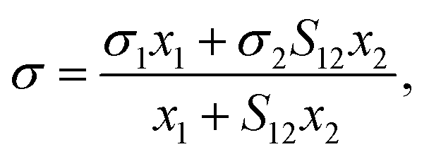 | (4) |
The pure component surface tensions σi in eqn (4) are temperature dependent. Shardt et al.33 and Tahery et al.34 showed that fit parameters of the Connors–Wright model and Shereshefsky model35 are approximately temperature independent for many binary aqueous systems with organic solutes. Since the Eberhart model is mathematically equivalent to the Shereshefsky model,18 it can be concluded that S12 is also constant with temperature for many systems. For the remainder of this study, we focus on modelling the surface tension at room temperature.
The Eberhart model is a simplified version of the Sigmoid model, which was derived by Kleinheins et al.18 as
 | (5) |
2.2 The ideal multi-component Eberhart model
The Eberhart model has been recently found to be a simple case of the Connors–Wright model with aij = bij = 1 − 1/Sij, where aij and bij are the fit parameters of the Connors–Wright model.18,33 This relationship was used to derive a multi-component Eberhart model from the existing multi-component Connors–Wright model.32 The Connors–Wright model, in turn, was found to be mathematically equivalent to the Chunxi model,31 which was derived from a Gibbs free energy expression of the bulk and surface phases. A more detailed derivation is described in the ESI† in Section S2. The resulting multi-component Eberhart model reads as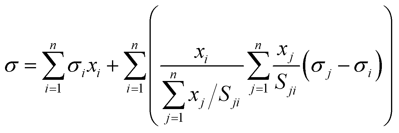 | (6) |
| Sii = 1, Sji = 1/Sij. | (7) |
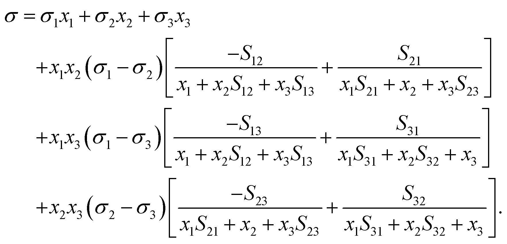 | (8) |
In principle, eqn (4), (6) and (8) are symmetrical, in the sense that the mixture components can be numbered in any order, and the relationship between the separation factor Sij for differently-ordered binary mixtures is given by eqn (7). The model is applicable to any solution containing water, salts, organic and/or amphiphilic substances. In the following, we will restrict the validation to data of aqueous solutions because of their relevance for atmospheric systems. For consistency throughout this study, we will refer to water as subscript 1 and number the solutes based on their surface partitioning S1i, from high S1i (strong partitioning) to low S1i (weak partitioning).
2.3 Consideration of non-ideality and synergism
In the literature the keywords non-ideality and synergism are often used when describing the surface tension data of systems with more than one solute. Multiple definitions of these terms can be found that may relate to very different phenomena. For example, synergistic effects in lowering the surface tension of a mixture should not be confused with synergism in wetting properties36 or synergism in foam stability.37 In this study we define the following terms:As a result of the inherent assumptions made in the derivation of eqn (6) (i.e., eqn (1)–(3)), this model cannot be expected to model any of the described non-idealities or synergistic effects. Due to the strong non-ideality found in systems containing surfactants and salts and due to the high relevance of such systems, e.g. for atmospheric sciences, here we explore the possibility to extend eqn (6) to capture non-ideality related to salting-out.
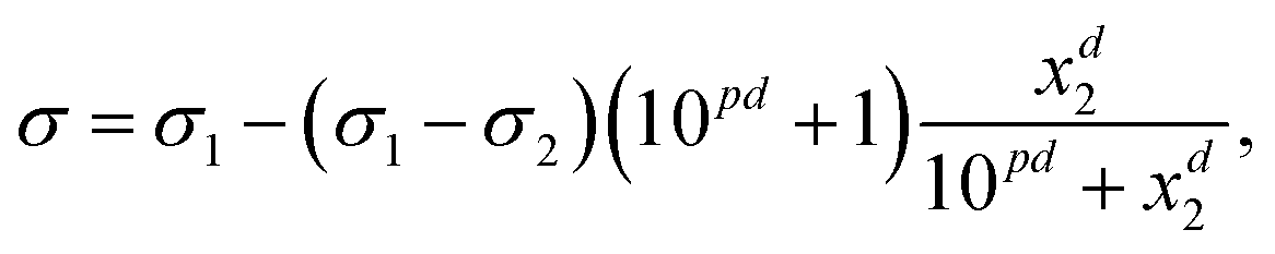
To model bulk non-ideality and partitioning synergism caused by salting-out, we suggest the following simple semi-empirical approach. Depending on the concentration of salt (here xj), the partitioning of less polar co-solutes (here e.g. a surfactant i) in water (1) is changed, which can be expressed by Snon-ideal1i = f(xj,S1i). We formulate this dependency as a simple linear equation
| Snon-ideal1i = S1i(1 + xjBSOij), | (9) |
Experimental data show that the presence of salts also results in surface non-ideality and slight surface synergism.40 In water–surfactant mixtures, a minimum surface tension is reached at the so-called critical micelle concentration (CMC) which is typically marked by a sudden change in slope in the surface tension–concentration curves, followed by constant surface tension. At the CMC, the surface reaches its maximum coverage in surfactant molecules. Further increasing the concentration of surfactant in the bulk leads to the formation of micelles. If salts are present, the CMC is not only shifted to lower concentrations (partitioning synergism) but also, a lower surface tension can be reached at the CMC, potentially due to reorientation or change in packing of the surfactant molecules at the surface.
To model this effect with the Eberhart model, eqn (1) has to be modified. Under the simple assumptions of the Eberhart model, a hypothetical complete coverage of the surface with surfactant molecules results in a surface mole fraction of the surfactant of xsurfi = 1, independent of the orientation or packing density of the surfactant molecules at the surface. Therefore, to achieve a lower surface tension than the surface tension of the pure surfactant σi with eqn (1), we suggest to perturb σi as a function of composition. To represent surface synergism caused by salts we make σi a function of the salt concentration and a fit parameter. Analogously to eqn (9), we suggest the linear equation
| σnon-ideali = σi(1 − xjASOij), | (10) |
Surface synergism and partitioning synergism have also been observed in mixtures of two surfactants in water.40,41 For such systems, the processes leading to synergism are different to the ones of surfactant–salt mixtures. While the salt is supposed to remain mainly in the bulk, the two surfactants are expected to partition both to the surface leading to synergistic (or competitive, or antagonistic) surface non-ideality. At full coverage of the surface, mixed micelles start to form in the bulk. Therefore, in the following we distinguish salting-out (SO) non-ideality from mixed-micelle (MM) non-ideality.
To model non-ideality and synergism of a system with two MM forming solutes i and j, we suggest to perturb S1i, S1j, σi, and σj as a function of composition. We further assume that the perturbation is largest when xi = xj, i.e. when the number of paired surfactant molecules is maximized. We define a new molar fraction xMMij, which expresses the fraction of paired surfactant molecules in the total number of surfactant molecules:
 | (11) |
 | (12) |
 | (13) |
For both SO non-ideality and MM non-ideality, Aij > 0 and Bij > 0 represent synergistic non-ideality, while a Aij < 0 and Bij < 0 represent competitive or antagonistic behaviour. In this study, we determine Aij and Bij by fitting to ternary surface tension data, as described next in Section 3.
To consider non-ideality in systems containing more than two solutes, all pairwise solute–solute interactions following the equations in this section should be taken into account. It is assumed that interactions involving three or more solute species are of minor importance and therefore such multi-solute interactions are not considered in this model. Two examples of modelling quaternary systems will be shown in Section 4.6.
3 Methods: determination of parameters
The model described in Section 2 was tested on experimental surface tension data from literature. An overview of all surface tension data of ternary and multi-component aqueous solutions found in the literature is given in the Tables S1–S7 in the ESI.† The measurement technique, temperature, and source data format of the systems that were modelled in this study are reported in Table S10 in the ESI.† To calculate the surface tension of a multi-component mixture with eqn (6), (9), and (10) the following quantities are needed:(1) The mole fraction xi of all mixture constituents for which σ should be calculated
(2) The pure liquid surface tension σi of all mixture constituents
(3) The separation factors Sij of all pairwise combinations of all mixture constituents, noting that Sij = 1 when there is a simple linear surface tension relationship with mole fraction
(4) The bulk non-ideality factor Bij and the surface non-ideality factor Aij for all relevant pairwise combinations for non-ideal mixtures, noting that Bij and Aij are equal to 0 in the absence of non-idealities or synergisms.
For the conversion between different concentration units (e.g. molar concentration in mol L−1 to unitless mole fraction) the molecular weight of the substances and the density of the solution must be known. For the calculation of the density of the solution, ideal mixing of the volume V was assumed  , except for the system water–CTAB–ethanol, where the density of the water–ethanol mixture was used42 and for the systems containing only surfactants as solutes, where the volume of the surfactants was neglected (dilute solution assumption). Table S11 in the ESI† summarizes the molar masses and densities that have been used for the investigated mixtures in this study.
The quality of the surface tension fits and predictions depends strongly on the choice of σi. It was found that a better fit or prediction was achieved when taking the σi values from the same source as the surface tension values σ of the mixed systems, since the measurement of σi may be subject to the same biases as the rest of the data (e.g. temperature biases). As a result, σi of a substance can exhibit different values when data from different sources are used. If σwater was not reported in the source publication, it was calculated for the measurement temperature with IAPWS–IF97.43 For NaCl, σNaCl = 169.73 mN m−1 was used, based on a temperature extrapolation to 25 °C from molten NaCl measurements.44 Analogously, σKCl = 153.74 mN m−1 and σ(NH4)2SO4 = 184.97 mN m−1 were used for KCl45 and (NH4)2SO4,46 respectively. The surface tension of pure glutaric and oxalic acid was determined by fitting the binary Eberhart model (eqn (4)) to binary water–glutaric acid and water–oxalic acid data. For surfactants, the lowest measured value in binary water–surfactant mixtures was taken for σi.
The binary separation factors Sij were determined by fitting eqn (4) to binary data, if available. If possible, binary data was taken from the same source as the ternary data to be modelled. The binary fits for all systems analyzed in this study are shown in Section S5 in the ESI.† For the prediction of the surface tension of a ternary water (1) + solute (2) + solute (3) mixture, the multi-component Eberhart equation (eqn (6)) requires not only the separation factors with water S1i, but also the separation factor of the water-free solute–solute mixture S23. Many solutes analyzed in this study are solid substances at room temperature. In this case, the surface tension of the water-free binary mixture refers to a hypothetical supercooled liquid state and thus cannot be measured in bulk measurements. In this case when no binary data to fit S23 was available it was determined by fitting to ternary surface tension data. In many cases, the ternary surface tension data of these systems covers only the dilute concentration range and as a result S23 is hardly constrained by experimental data, which leads to a large fit parameter uncertainty. If the choice of S23 had no noticeable influence on the fit or prediction quality, it was set to S23 = 1 corresponding to a simple linear surface tension relationship. Lastly, when applicable, Bij and Aij require fitting to ternary surface tension data, too.
To conclude, depending on the system and the availability of data, the following fitting steps are required:
• Fitting to binary data: all Sij parameters (and σi, if unknown).
• Fitting to ternary data: if the system is behaving non-ideally, fitting of Aij and Bij (or set Aij and Bij to zero if ideality is assumed). If binary data i − j is not available, fit Sij to ternary data (or set to unity if linear mixing can be assumed).
Fit parameters were determined by minimizing nonlinear least squares using the curve_fit() function (with default settings) of the module optimize of the Python package SciPy.47 For each fit parameter i, the 95% confidence interval (CI95,i) was estimated by
 | (14) |
4 Results and discussion
Fig. 1 gives an overview of the structure of the following sections. Solutes were grouped into salts (inorganic electrolytes), organics (small organic substances), and surfactants (large amphiphilic substances).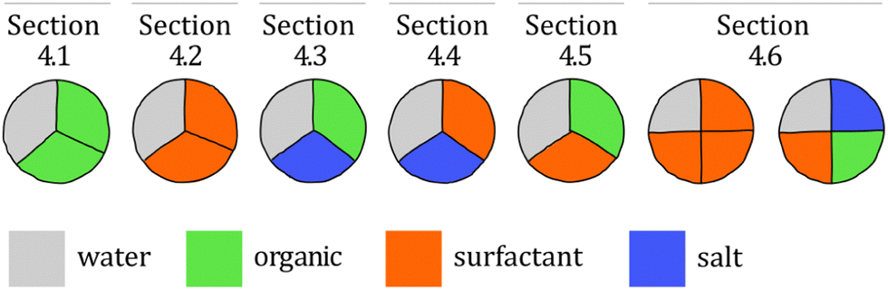 | ||
| Fig. 1 Illustration of the structure of the results sections. For example, Section 4.1 shows results of ternary mixtures of water with two organic solutes. | ||
Not all data sets found in literature are equally complete. Therefore, in the following, we show results for selected systems that cover a broad range of substance types and compositions with a large number of data points that showcase the strengths and limitations of the model well. An overview of all modelled ternary systems, the fit parameters and the model accuracy is given in Table 1.
| System water (1) + | n p | σ 1 (mN m−1) | σ 2 (mN m−1) | σ 3 (mN m−1) | S 12 (±CI95) | S 13 (±CI95) | S 23 (±CI95) | A 23 (±CI95) | B 23 (±CI95) | RMSE (mN m−1) | Δσmax (mN m−1) |
|---|---|---|---|---|---|---|---|---|---|---|---|
| Acetonitrile (2) + 1,2-ethanediol (3)48 | 52 | 72.06 | 28.20 | 48.22 | 22.23 | 5.34 | 0.33 | 0 | 0 | 1.14 | 2.53 |
| (1.66) | (0.10) | (0.03) | |||||||||
| n-Butyl acetate (2) + methanol (3)49 | 48 | 71.40 | 23.60 | 21.59 | 228.98 | 7.02 | 0.39 | 0 | 0 | 0.41 | 0.95 |
| (121.49) | (0.67) | (0.05) | |||||||||
| Brij35 (2) + SDS (3)50 | 60 | 72.00 | 30.52 | 32.95 | 1.5 × 10⁶ | 5.7 × 10⁴ | 1 | 0 | 0 | 2.17 | 5.50 |
| (1.2 × 10⁵) | (7.7 × 10³) | ||||||||||
| TX100 (2) + CTAB (3)51 | 55 | 72.80 | 33.30 | 37.80 | 2.9 × 10⁶ | 2.4 × 10⁵ | 1 | −0.15MM | 2.33MM | 1.57 | 3.57 |
| (4.9 × 10⁵) | (6.1 × 10⁴) | (0.04) | (0.56) | ||||||||
| CTAC (2) + SDS (3)40 | 41 | 73.37 | 38.61 | 34.06 | 1.4 × 10⁵ | 2.3 × 10⁴ | 1 | 0.18MM | −0.80MM | 3.38 | 11.36 |
| (5.9 × 10⁴) | (1.2 × 10⁴) | (0.08) | (0.10) | ||||||||
| DDAO (2) + SDS (3)41 | 53 | 70.00 | 31.63 | 36.16 | 2.9 × 10⁵ | 2.1 × 10⁴ | 1 | 0.36MM | 1.10MM | 3.82 | 9.88 |
| (1.1 × 10⁵) | (8.9 × 10³) | (0.07) | (0.54) | ||||||||
| TX114 (2) + SDS (3)40 | 73 | 73.60 | 30.14 | 34.06 | 1.7 × 10⁶ | 2.3 × 10⁴ | 1 | 0 | 0 | 2.89 | 6.97 |
| (5.2 × 10⁵) | (1.2 × 10⁴) | ||||||||||
| Glutaric acid (2) + NaCl (3)52 | 30 | 73.00 | 53.71 | 169.73 | 92.45 | 0.79 | 1 | 0 | 34.00SO | 2.24 | 6.44 |
| (1.44) | (33.83) | (0.09) | (12.32) | ||||||||
| Succinic acid (2) + NaCl (3)53 | 16 | 71.60 | 52.85 | 169.73 | 31.80 | 1.06 | 1 | 0 | 19.72SO | 0.30 | 0.63 |
| (15.21) | (30.57) | (0.14) | (1.92) | ||||||||
| Glutaric acid (2) + (NH4)2SO4 (3)40 | 22 | 73.78 | 50.20 | 184.97 | 76.95 | 1.1054 | 1 | 0 | 191.48SO | 3.19 | 6.54 |
| (1.84) | (17.94) | (0.08) | (90.40) | ||||||||
| Malonic acid (2) + (NH4)2SO4 (3)55 | 16 | 72.58 | 46.01 | 184.97 | 15.53 | 1.1054 | 1 | 0 | 39.02SO | 1.14 | 2.42 |
| (2.02) | (3.79) | (0.08) | (15.78) | ||||||||
| TX100 (2) + NaCl (3)40 | 60 | 73.53 | 31.52 | 169.73 | 1.6 × 10⁶ | 0.8856 | 1 | 4.08SO | 29.84SO | 3.26 | 8.84 |
| (2.9 × 10⁵) | (0.03) | (9.16) | |||||||||
| SDS (2) + NaCl (3)57 | 100 | 72.26 | 38.83 | 169.73 | 2.8 × 10⁴ | 0.8856 | 1 | 22.36SO | 2.8 × 10³![[thin space (1/6-em)]](https://www.rsc.org/images/entities/char_2009.gif) SO SO |
3.83 | 8.13 |
| (9.9 × 10³) | (0.03) | (4.2 × 10²) | |||||||||
| CTAB (2) + NaCl (3)58 | 453 | 70.00 | 36.92 | 169.73 | 2.3 × 10⁵ | 0.8856 | 3.6 × 10⁻⁷ | 1.24SO | 2.7 × 10⁴SO |
2.64 | 7.20 |
| (4.8 × 10⁴) | (0.03) | (3.9 × 10⁻⁷) | (1.7 × 10³) | ||||||||
| CTAB (2) + KCl (3)59 | 149 | 72.40 | 36.59 | 153.74 | 2.4 × 10⁵ | 0.62 | 1 | −3.08SO | 2.3 × 10⁴SO |
2.26 | 7.18 |
| (4.8 × 10⁴) | (0.24) | (2.37) | (2.1 × 10³) | ||||||||
| TX100 (2) + (NH4)2SO4 (3)40 | 33 | 73.53 | 31.52 | 184.97 | 1.6 × 10⁶ | 1.1054 | 1 | 6.20SO | 58.11SO | 3.11 | 6.77 |
| (2.9 × 10⁵) | (0.08) | (31.72) | |||||||||
| TX100 (2) + glutaric acid (3)40 | 101 | 73.70 | 31.52 | 50.20 | 1.6 × 10⁶ | 76.95 | 1 | 0 | 0 | 3.22 | 8.72 |
| (1.84) | (2.9 × 10⁵) | (17.94) | |||||||||
| TX100 (2) + oxalic acid (3)40 | 63 | 73.60 | 31.52 | 65.49 | 1.6 × 10⁶ | 100.59 | 1 | 0 | 92.99SO | 2.48 | 6.48 |
| (2.45) | (2.9 × 10⁵) | (61.78) | (57.38) | ||||||||
| SDS (2) + oxalic acid (3)40 | 45 | 73.60 | 34.06 | 65.49 | 2.3 × 10⁴ | 100.59 | 1 | 0 | 4.4 × 10³SO |
2.86 | 8.60 |
| (2.45) | (1.2 × 10⁴) | (61.78) | (9.8 × 10²) | ||||||||
| CTAB (2) + ethanol (3)42 | 243 | 72.80 | 37.00 | 23.22 | 2.4 × 10559 |
20.6060 | 1 | 0 | 0 | 3.30 | 8.01 |
| (4.8 × 10⁴) | (1.89) | ||||||||||
| Brij35 (2) + glutaric acid (3)40 | 80 | 73.66 | 44.91 | 50.20 | 3.0 × 10⁶ | 76.12 | 1 | 0 | 0 | 2.33 | 5.14 |
| (1.81) | (7.1 × 10⁵) | (17.37) | |||||||||
| CTAC (2) + oxalic acid (3)40 | 49 | 73.60 | 38.61 | 65.49 | 1.4 × 10⁵ | 100.59 | 1 | 0 | 1.0 × 10⁴SO |
8.57 | 22.16 |
| (2.45) | (5.9 × 10⁴) | (61.78) | (7.9 × 10³) |
4.1 Water–organic–organic systems
Liquid mixtures containing organic substances, whether atmospheric aerosol particles, crude oil or alcoholic beverages, typically contain a mixture of different organic substances rather than a single species. The surface tension of such mixtures plays an important role in various applications, such as the efficient operation of distillation trays.61 Here, we analyze the surface tension of solutions containing water and two organic species.In Fig. 2, the results for the system water–acetonitrile–1,2-ethanediol are shown. Due to the full solubility of this system, the data covers the whole concentration range including all binary boundaries. Fitting the separation factors Sij to the binary data with eqn (4) allows to predict the ternary data points without any additional fit parameter. As can be seen from the low root mean squared error (RMSE) of 1.14 mN m−1 and the low maximum error in surface tension Δσmax = 2.53 mN m−1, the prediction of the ternary data points is very accurate for this system.
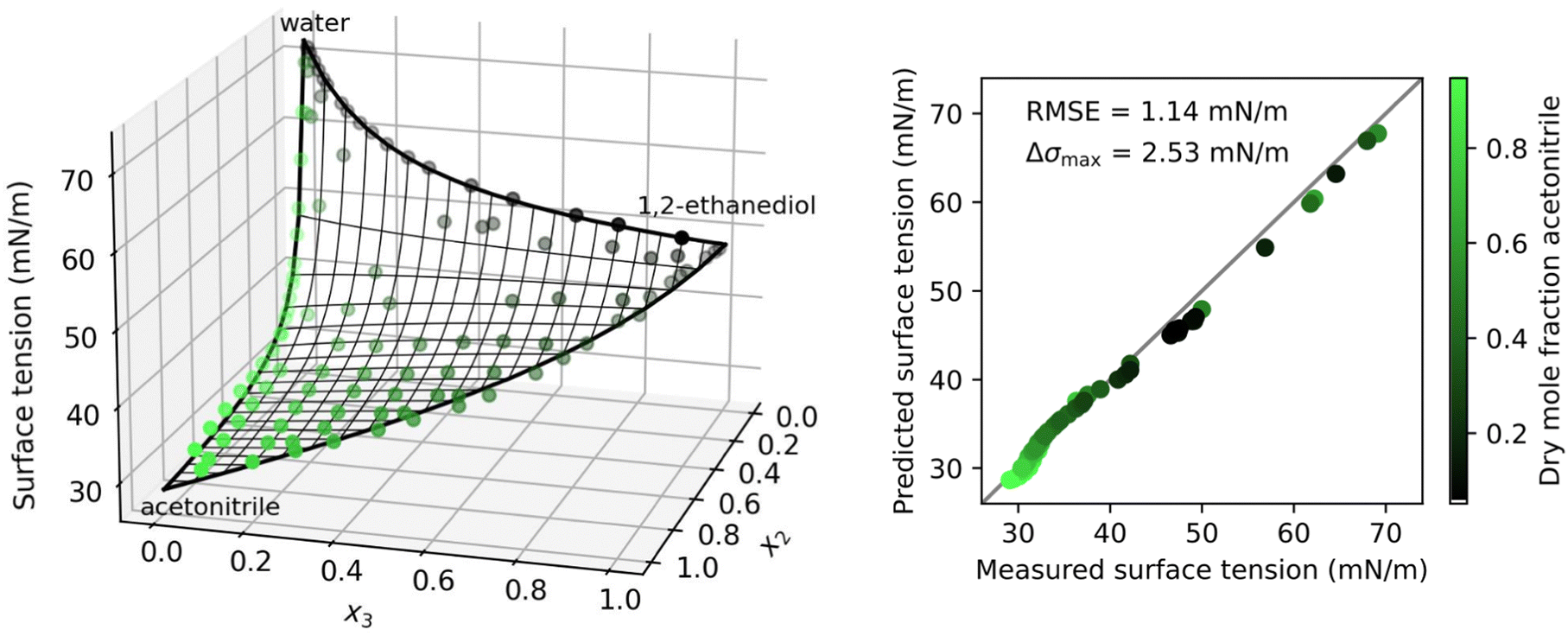 | ||
| Fig. 2 Surface tension of the ternary system water (1) + acetonitrile (2) + 1,2-ethanediol (3) at 25 °C as a function of the mole fractions xi. Left: Symbols show measurements by Rafati et al.,48 thick black lines: binary fits (eqn (4)), thin black lines: ternary prediction (eqn (8)). Right: Error plot showing the predicted vs. measured surface tension of the ternary data points, the root mean squared error (RMSE), and the maximum error in σ (Δσmax). Colors show the dry mole fraction of acetonitrile as x2/(x2 + x3). | ||
Fig. 3 shows a system with a solubility gap and therefore incomplete data. N-Butyl acetate (2) has a very low solubility in water (1) and therefore the separation factor S12 could not be determined from fitting to binary data. Instead, it was fitted to the ternary data. The resulting binary water–n-butyl acetate surface tension is shown as a dashed line in Fig. 3. With this approach, the ternary data could be modelled very accurately.
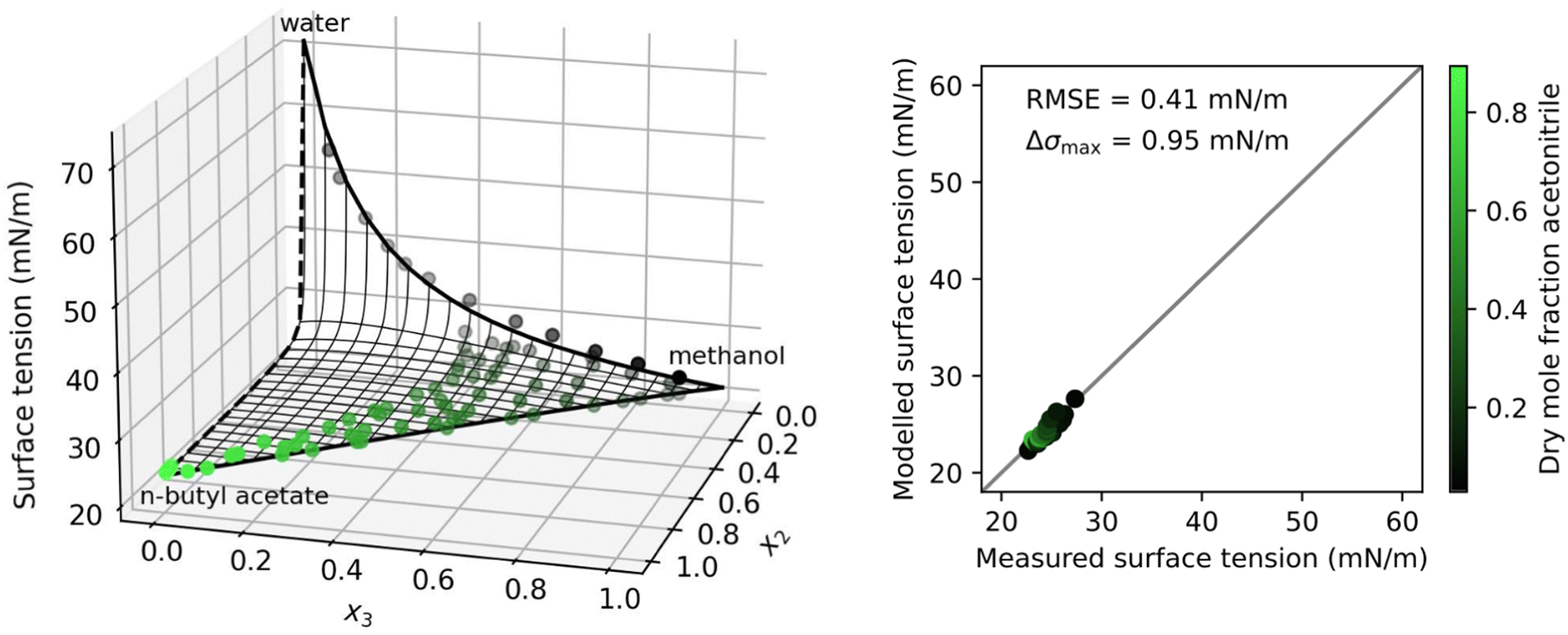 | ||
| Fig. 3 Surface tension of the ternary system water (1) + n-butyl acetate (2) + methanol (3) at 30 °C as a function of the mole fractions xi. Left: Symbols show measurements by Santos et al.,49 thick solid black lines: binary fits (eqn (4)), thick black dashed line: fitted to ternary data, thin black lines: ternary prediction (eqn (8)). Right: Error plot showing the predicted vs. measured surface tension of the ternary data points, the root mean squared error (RMSE), and the maximum error in σ (Δσmax). Colors show the dry mole fraction of n-butyl acetate as x2/(x2 + x3). | ||
In Shardt and Elliott33 and Kleinheins et al.18 it was found that the Connors–Wright model yielded slightly better surface tension fits than the Eberhart and Shereshefsky models for a number of binary aqueous solutions of water soluble organic substances. Therefore, we tested if the multi-component Connors–Wright model32 also is more accurate than the multi-component Eberhart model for the ternary systems shown in this section. It was found that the RMSE of the system water–acetonitrile–1,2-ethanediol could be further lowered from 1.14 mN m−1 to 1.00 mN m−1 by the Connors–Wright model, partly due to a better binary acetonitrile–1,2-ethanediol fit, and the RMSE of the system water–n-butyl acetate–methanol could be further lowered from 0.41 mN m−1 to 0.33 mN m−1, mostly due to a better binary water–methanol fit (more details are given in Section S4 in the ESI†). The fact that the binary Connors–Wright model has one fit parameter more than the binary Eberhart model allows for better fits for some organic substances. However, no better performance was found for surfactant solutions, neither in binary mixtures18 nor in the ternary systems examined in this study. Furthermore, the additional fit parameter makes the Connors–Wright model less robust against scatter in experimental data. For these reasons, the Eberhart model was considered more appropriate and the multi-component Connors–Wright model was not investigated further.
4.2 Water–surfactant–surfactant systems
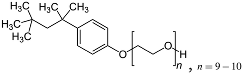
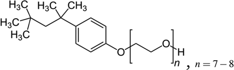
Mixtures of surfactants are often found in consumer and industrial formulations, from household cleaning products to large scale spray coating mixtures. For example, emerging fluorine-free fire fighting foams would benefit from synergistic mixtures of surfactants.2 In this section, we present results for the surface tension of various pairs of surfactants in water, including nonionic (Brij35, TX100, TX114), anionic (SDS), cationic (CTAB, CTAC), and zwitterionic surfactants (DDAO). The full names and the structures of all surfactants in this study are shown in Table 2.| Abbr. | IUPAC name | Type | S | CMC | σ CMC | Structure |
|---|---|---|---|---|---|---|
| Brij35 | 2-(Dodecyloxy)ethan-1-ol | Nonionic | 2 × 10⁶ | 1 × 10⁻⁴ | 30–45 |
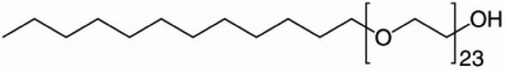
|
| TX100 | 2-[4-(2,4,4-Trimethylpentan-2-yl)phenoxy]ethanol | Nonionic | 2 × 10⁶ | 2 × 10⁻⁴ | 32–33 |
|
| TX114 | 2-[4-(2,4,4-Trimethylpentan-2-yl)phenoxy]ethanol | Nonionic | 2 × 10⁶ | 2 × 10⁻⁴ | 30 |
|
| SDS | Sodium dodecyl sulfate | Anionic | 4 × 10⁴ | 8 × 10⁻³ | 33–39 |
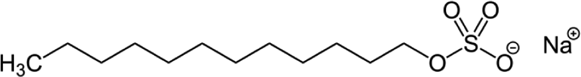
|
| CTAB | N,N,N-Trimethylhexadecan-1-aminium bromide | Cationic | 2 × 10⁵ | 1 × 10⁻³ | 37–38 |
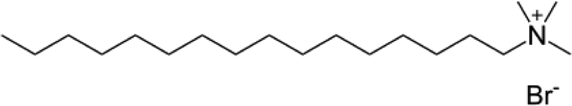
|
| CTAC | N,N,N-Trimethylhexadecan-1-aminium chloride | Cationic | 1 × 10⁵ | 1 × 10⁻³ | 39 |
|
| DDAO | N,N-Dimethyldodecan-1-amine N-oxide | Zwitterionic | 3 × 10⁵ | 1 × 10⁻³ | 32 |
|
Fig. 4 shows results of four different types of water–surfactant–surfactant systems. For each system, S12 and S13 were obtained from binary water–surfactant fits shown in Section S5.2 in the ESI.† It can be noticed that the slope in the surface tension before the CMC of some pure surfactants (e.g., CTAB) and the typical abrupt change in slope around the CMC cannot be reproduced well with the Eberhart model, due to its sigmoidal nature and due to the lack of a parameter influencing the slope (see also Section S1 in the ESI†). This leads to errors of up to ≈10 mN m−1 in the binary fits and systematic errors from the sigmoidal shape that propagate to the ternary surface tension modelling (e.g., right panel, second row in Fig. 4 and Fig. S12 in the ESI†).
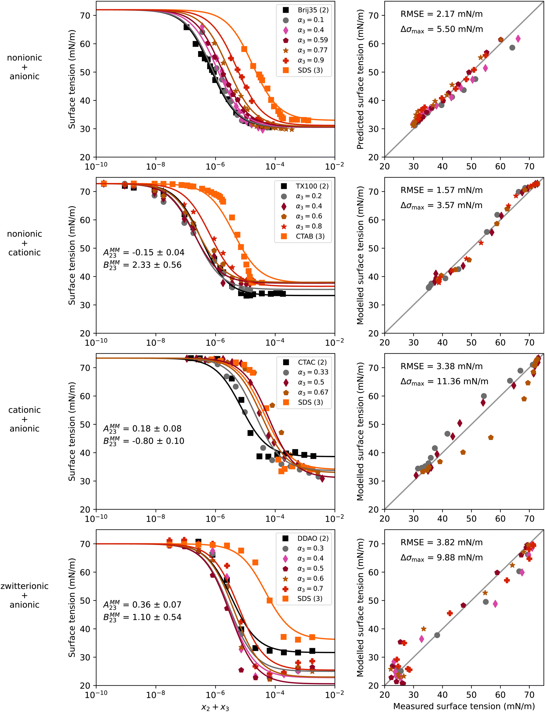 | ||
| Fig. 4 Surface tension of four water–surfactant–surfactant systems as a function of the solute mole fraction x2 + x3. Left panels show experimental data (symbols) and model results (solid lines) from eqn (4), (8), (12), and (13). Right panels show the error in predicted surface tension for all ternary data points. The dry mole fraction α3 is defined as x3/(x2 + x3). First row: Water (1) + Brij35 (2) + SDS (3), T = 25 °C, data from Zakharova et al.50 Second row: Water (1) + TX100 (2) + CTAB (3), T = 20 °C, data from Szymczyk and Janczuk.51 Third row: Water (1) + CTAC (2) + SDS (3), T = 24 °C, data from El Haber et al.40 Fourth row: Water (1) + DDAO (2) + SDS (3), T = 25 °C, data from Tyagi et al.41 Binary fits are shown in Fig. S7 in the ESI.† | ||
We tried to fit S23 to the ternary data, yet, this fitting parameter proved to be completely unconstrained, since experimental data in this concentration range is lacking. Therefore, S23 = 1 was chosen for all systems, corresponding to a linear mixing of the water-free surface tension.
For the nonionic–anionic system water–Brij35–SDS, the ternary surface tension could be predicted closely without non-ideality factors (see first row in Fig. 4). A second ternary mixture containing a nonionic and an anionic surfactant (water–TX114–SDS, see Fig. S12 in the ESI†) confirmed the capability of the Eberhart model to predict surface tensions for ternary water–nonionic–anionic systems from binary data alone. The fact that the ideal Eberhart model is used without additional parameters means that these systems show ideal behaviour following the definitions given in Section 2.3. Yet, plotting the CMC versus the surfactant dry mole fraction α does not result in a linear relationship as shown in El Haber et al.,40 which in that study is referred to as non-ideality. Analyzing the system with the Eberhart model shows that the CMC of the mixed systems can be described without taking any interactions between the two surfactants into consideration, which we judge as ideal behavior here.
In contrast to these ideal systems, the other three systems in Fig. 4 could not be predicted well when assuming ideality, as shown in Fig. S13 in the ESI.† The non-ideal behaviour of these system could, however, be modelled by using eqn (12) and (13). The parameters AMM23 and BMM23 that were obtained by fitting to the ternary data are shown in the left panels of Fig. 4. The negative sign of AMM23 for the water–TX100–CTAB mixture indicates a slight competitive surface non-ideality for this nonionic–cationic system. In contrast, the cationic–anionic water–CTAC–SDS and the zwitterionic–anionic water–DDAO–SDS systems show surface synergism as indicated by the positive sign of AMM23. Partitioning synergism is observed for water–TX100–CTAB and water–DDAO–SDS, while water–CTAC–SDS shows partitioning antagonism, as reflected by the positive and negative BMM23 values, respectively.
These findings are confirmed by studies showing that solutions containing vesicle forming mixtures of cationic and anionic (‘catanionic’) surfactants behave strongly non-ideally, compared to solutions of the cationic or the anionic surfactant alone.62,63 Also, mixtures with zwitterionic surfactants have been found to behave non-ideally before.41 In contrast, solutions with cationic and nonionic surfactants, like water–TX100–CTAB in our case, are less known to be non-ideal. This example highlights the strength of the model as an analytical tool for the examination of mixtures for non-ideality.
4.3 Water–organic–salt systems
Water–organic–salt systems are of particular interest in atmospheric sciences, where mixtures of dicarboxylic acids and inorganic salts are often chosen as model systems to represent complex atmospheric aerosol particles. Therefore, surface tension data of water–organic–salt systems available in the literature is dominated by dicarboxylic acid–salt mixtures. The results for four such systems are shown in Fig. 5. They contain a dicarboxylic acid (malonic, succinic, or glutaric acid) and NaCl or (NH4)2SO4.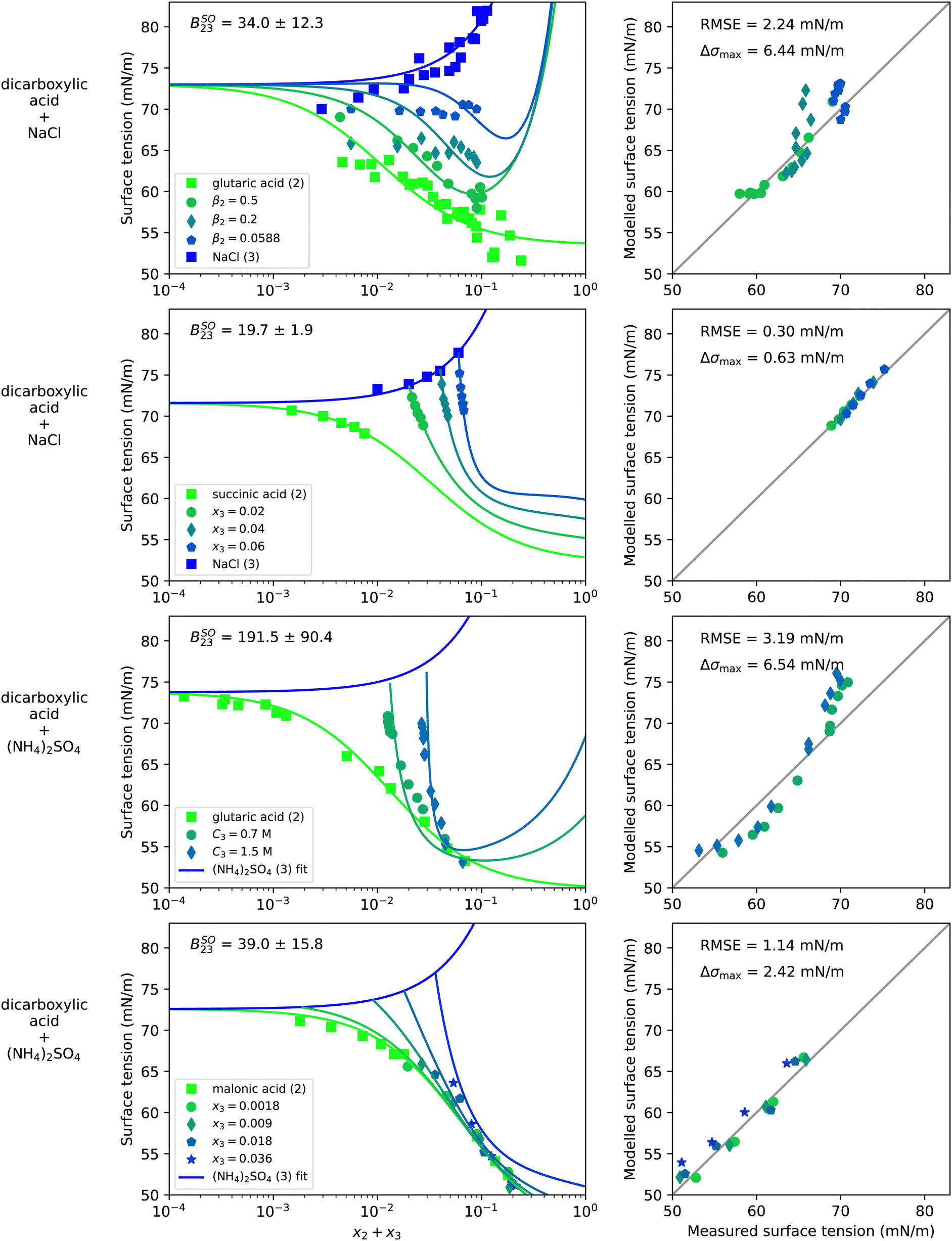 | ||
| Fig. 5 Surface tension of four water–organic–salt systems as a function of the solute mole fraction x2 + x3. Left panels show experimental data (symbols) and model results (solid lines) from eqn (4), (8) and (9). Right panels show the error in predicted surface tension for all ternary data points. The dry mass fraction β2 is defined as m2/(m2 + m3) where m is the mass. C3 is the molar concentration of substance 3 in mol Lsolution−1 (M). First row: Water (1) + glutaric acid (2) + NaCl (3), T = 25 °C, data from Miles et al.52 Second row: Water (1) + succinic acid (2) + NaCl (3), T = 25 °C, data from Vanhanen et al.53 Third row: Water (1) + glutaric acid (2) + (NH4)2SO4 (3), T = 24 °C, data from El Haber et al.40 Fourth row: Water (1) + malonic acid (2) + (NH4)2SO4 (3), T = 21 °C, data from Booth et al.55 Binary fits are shown in Fig. S8 in the ESI.† | ||
Since the data cover mostly only the dilute concentration range, S23 is barely constrained and therefore set to unity. The choice of S23 = 1 leads to the strong upticks in the modelled curves that can be seen at high solute concentrations in the systems containing glutaric acid. Choosing a lower value of S23 instead would lead to less of an uptick, a lower BSO23 value and a slightly worse fit quality for water–glutaric acid–NaCl, as shown in Fig. S14 in the ESI.† However, since not enough experimental data are available at high solute concentrations, it is not clear which value of S23 represents this system best.
Due to the presence of salts in these systems, the bulk non-ideality factor for salting-out BSO23 was fitted to the ternary data. The resulting value is shown in Fig. 5 in the upper left corner of the left plots. For comparison, Fig. S15 in the ESI† displays the results with BSO23 = 0 showing that the fit quality could be strongly improved by adding the non-ideality parameterization to the model.
Comparing the salting-out factors for systems with the same salt, it can be seen that a higher BSO23 was found for the dicarboxylic acid with the longer hydrocarbon chain. This makes sense since the longer non-polar hydrocarbon chain is expected to experience a stronger repulsion by the ions leading to a stronger salting-out of the organic molecules. Furthermore, for glutaric acid, a higher BSO23 was found in mixture with (NH4)2SO4 than with NaCl. It is well known that activity coefficients in bulk phases containing electrolytes depend on the ionic strength of the solution, which is proportional to the square of the ion charge. (NH4)2SO4 in aqueous solution produces double charged sulfate ions, while NaCl only produces single charged sodium and chloride ions. This might explain why a higher BSO23 was found for (NH4)2SO4 than for NaCl containing systems.
The modelled water–glutaric acid–NaCl system shows large deviations at low concentrations. This has also been observed by Miles et al.52 and was explained by challenges in the experimental setup. The water–succinic acid–NaCl system could be modelled very accurately, but the data are limited to a very small concentration range due to the low solubility of succinic acid in water. Also in the two systems with (NH4)2SO4 only limited experimental data were available. In the system water–glutaric acid–(NH4)2SO4, the right panel shows systematic errors of the modelled surface tension. The two experimental data points with x2 = 0 reported by El Haber et al.40 are lower than the binary data measured by Hyvarinen et al.,54 which was used for the binary (NH4)2SO4–water fit. This discrepancy in the experimental data leads to the higher modelled surface tension in the upper part of the right panel of that system. The bias in the experimental data translates to a fitted BSO23 that is too high, leading to the lower modelled surface tension in the lower part of the right panel. Clearly, more ternary water–organic–salt surface tension data including systems with liquid soluble organic substances (e.g. alcohols) would help to further test the potential of this model approach and to constrain S23 and BSO23 better.
4.4 Water–surfactant–salt systems
Mixtures of surfactants and salts are of high importance for atmospheric aerosol sciences as well as for a number of industrial applications. Marine aerosol particles produced by sea spray were found to contain nonionic and ionic surfactants in addition to sea salt, which consists mostly of NaCl.13,64,65 In line with the interest in surfactant–NaCl systems, in this section we present results of a nonionic (TX100), an anionic (SDS), and a cationic (CTAB) surfactant each in solution with NaCl. In addition, we show CTAB in mixture with KCl and TX100 with (NH4)2SO4. The experimental and modelling results for the NaCl and KCl containing systems are shown in Fig. 6 and the system with (NH4)2SO4 is presented in Fig. S18 in the ESI.† In contrast to the systems shown before, these systems are plotted with x2 along the x-axis, as the data lines of constant salt concentration would appear as vertical lines on a x2 + x3 scale. For a better representation of the vertically-aligned data in the water–CTAB–KCl system, Fig. S16 in the ESI† shows the same data plotted once with x2 and once with x3 as the x-axis. Furthermore, the system water–CTAB–NaCl is shown enlarged and with a different coloring in Fig. S17 in the ESI† for a better differentiation between the data series.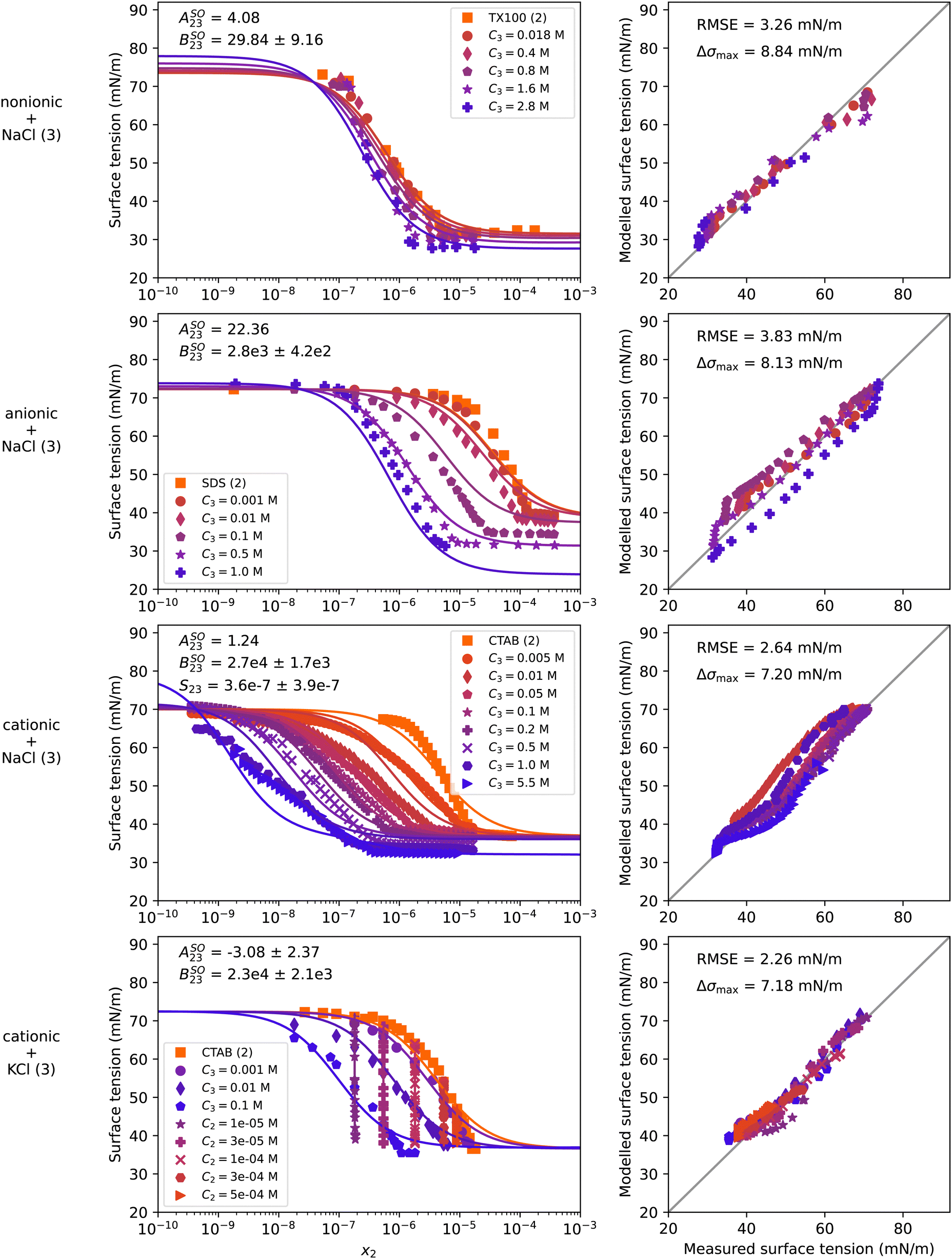 | ||
| Fig. 6 Surface tension of four water–surfactant–salt systems as a function of the surfactant mole fraction x2. Left panels show experimental data (symbols) and model results (solid lines) from eqn (4), (8), (9), and (10). Right panels show the error in predicted surface tension for all ternary data points. Ci is the molar concentration of substance i in mol Lsolution−1 (M). First row: Water (1) + TX100 (2) + NaCl (3), T = 24 °C, data from El Haber et al.40 Second row: Water (1) + SDS (2) + NaCl (3), T = 25 °C, data from Nakahara et al.57 Third row: Water (1) + CTAB (2) + NaCl (3), T = 21 °C, data from Qazi et al.58 Fourth row: Water (1) + CTAB (2) + KCl (3), T = 22 °C, data from Para et al.59 Binary fits are shown in Fig. S9 in the ESI.† | ||
S 23 was set to 1 for all systems except water–CTAB–NaCl, since the binary surfactant–salt surface tension of those systems could not be constrained with the given data. In contrast, the data points with 5.5 M NaCl of the water–CTAB–NaCl system were sufficiently concentrated to constrain S23 to a value of 3.6 × 10⁻⁷ for this system, although with a high uncertainty (see respective panel in Fig. 6). The small value of S23 means that in concentrated NaCl solutions, the presence of only small amounts of CTAB determine the surface tension of the solution. This is most likely the case for all water–surfactant–salt systems, leading to very small S23 values also for the other investigated systems; yet, as data to constrain this parameter are missing, S23 = 1 was chosen. More measurements at high salt concentrations might allow to determine generic or even parameterized S23 values for such systems.
For all systems, the addition of salt shifts the surface tension curve of the respective surfactant to lower concentrations. This salting-out effect is reflected in the model by a bulk non-ideality factor BSO23 > 0, which was retrieved by fitting to the ternary data and is displayed in the upper left of the panels in the left column. While for the nonionic surfactant (TX100) the salting-out is moderate (BSO23 = 29 ± 9), it is much stronger for the anionic and the cationic surfactants for the same salt (BSO23 = 2811 ± 420 and BSO23 = 2.7 × 10⁴ ± 1.7 × 10³). As KCl and NaCl are both alkali chlorides, adding either of them to CTAB leads to a similar salting-out effect as reflected by BSO23 having similar values. The addition of (NH4)2SO4 instead of NaCl to TX100 leads to a slightly higher salting-out factor of BSO23 = 58 ± 31 as shown in Fig. S18 in the ESI,† which is in line with the observations for the water–organic–salt systems. Neglecting non-ideality for this systems leads to poor model predictions (see Fig. S19 in the ESI†). For a general correlation of the salting-out factor with surfactant and salt type, more experimental data would need to be examined.
Besides the strong salting-out effect, surface synergism can be observed in all of the systems with NaCl evidenced by a lowering of the surface tension below the surface tension of the pure surfactant, which becomes more pronounced the more salt is present. To model the combined effect of salting-out and surface synergism, both eqn (9) and (10) were used together with eqn (8) to achieve the fit quality shown in Fig. 6. The surface non-ideality factor ASO23 was adjusted in such a way that the model reproduces the experimental data of the lowest plateau, except for water–CTAB–KCl, where ASO23 was fitted, since the C2 = 1 × 10⁻⁵ mol L−1 and C3 = 0.1 mol L−1 data are not self-consistent and show conflicting trends. In this system, a negative value was found for ASO23, but with a large uncertainty. While for the systems with NaCl the addition of the ASO23 parameter improved the RMSE noticeably, no improvement was found for the last system, so that ASO23 could also be set to zero (see Fig. S20 in the ESI†).
As for the systems in the previous sections, the binary fit to the water–surfactant data cannot reproduce the sharp bend at the CMC and the steep slope observed for the surface tension curves of SDS and CTAB. This leads to an error that propagates to the ternary modelling. Despite the limitations in reproducing the sharp bend at the CMC, the model captures the general trends in the surface tension curves well including the salting-out effects so that maximum errors remain below 10 mN m−1 for all systems. In addition, the model parameters can be used to inform the degree of salting out and synergism present for a given system.
4.5 Water–surfactant–organic systems
The surfactants found in atmospheric aerosol particles are usually in mixtures with other organic substances. Therefore, from an atmospheric science perspective, the interactions between surfactants and other organic solutes need to be understood. In Fig. 7, experimental data and model results of four water–surfactant–organic systems are shown. The first two rows show systems of the nonionic surfactant TX100 with a dicarboxylic acid (glutaric acid or oxalic acid). The third row shows the anionic surfactant SDS with oxalic acid. The last system contains a cationic surfactant (CTAB) and an alcohol (ethanol). For a better representation of the data at constant acid concentration (vertical lines) of the water–TX100–glutaric acid system, additional plots with x2 and x3 on the x-axis are shown in Fig. S21 in the ESI.† The strong upticks noticeable at high solute concentration in the first three systems shown in Fig. 7 are, again, a result of choosing S23 = 1, as discussed before in Section 4.3.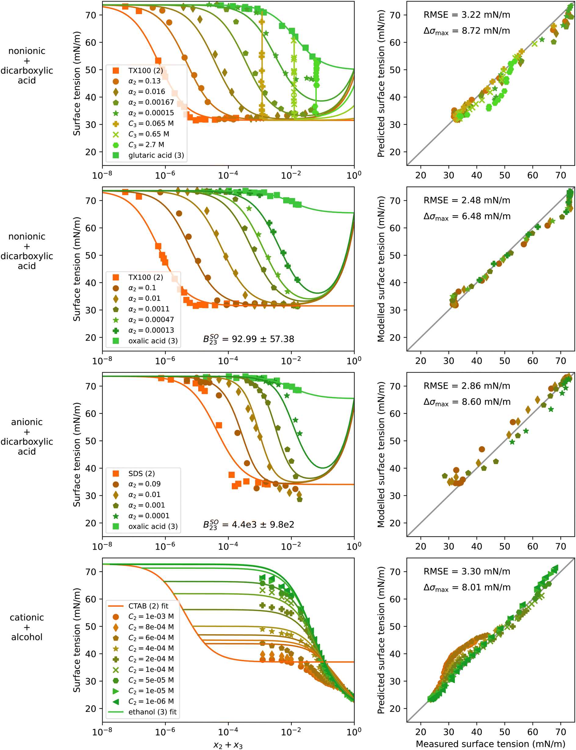 | ||
| Fig. 7 Surface tension of four water–surfactant–organic systems as a function of the solute mole fraction x2 + x3. Left panels show experimental data (symbols) and model results (solid lines) from eqn (4), (8), and (9). Right panels show the error in predicted surface tension for all ternary data points. The dry mole fraction α2 is defined as x2/(x2 + x3). Ci is the molar concentration of substance i in mol Lsolution−1 (M). First row: Water (1) + TX100 (2) + glutaric acid (3), T = 24 °C, data from El Haber et al.40 Second row: Water (1) + TX100 (2) + oxalic acid (3), T = 24 °C, data from El Haber et al.40 Third row: Water (1) + SDS (2) + oxalic acid (3), T = 24 °C, data from El Haber et al.40 Fourth row: Water (1) + CTAB (2) + ethanol (3), T = 20 °C, data from Bielawska et al.42 Binary fits are shown in Fig. S10 in the ESI.† | ||
The surface tension of the system water–TX100–glutaric acid can be predicted well from the binary fits and with S23 = 1 without any fitting to the ternary data over most of the concentration range. At the highest measured solute concentration, the model predicts a lower surface tension than what has been measured, which could be caused by competitive surface non-ideality. Applying eqn (10) to model the surface non-ideality of the water–TX100–glutaric acid leads to a negative Aij value, supporting the hypothesis of competitive surface behaviour. However, similar to the water–surfactant–surfactant systems, the model with non-ideality predicts unrealistic values at high concentrations and is not recommended to be used outside the measured data range (shown in Fig. S22 in ESI†). For comparison to the water–TX100–glutaric acid system, Fig. S23 in the ESI† shows the system water–Brij35–glutaric acid. This system could also be predicted well for most of the concentration range, but in contrast to the system with TX100, here a slight surface synergism was observed at high solute concentrations.
Furthermore, three systems containing oxalic acid were modelled: one with a nonionic surfactant (water–TX100–oxalic acid, Fig. 7), one with an anionic surfactant (water–SDS–oxalic acid, Fig. 7), and one with a cationic surfactant (water–CTAC–oxalic acid, Fig. S24 in ESI†). All three systems were found to exhibit salting-out bulk non-ideality, reflected by positive values for the fitted BSOij parameter. Assuming ideality instead (see Fig. S25 in ESI†) yielded a worse fit quality. Oxalic acid is a much stronger acid than glutaric acid and partly deprotonates in solution with water. The formed H+ and HC2O4− ions increase the ionic strength of the aqueous solution which might explain a salting-out behaviour in surface tension. The dissociation of oxalic acid is expected to be stronger at higher dilution while at high concentration, oxalic acid is not expected to deprotonate. Consequently, the salting-out effect must scale with dilution, an effect that cannot be modelled with the equations in this study. As a result, the surface tension is under- and overestimated at high and low oxalic acid concentration, respectively, which can be seen in the plots for water–SDS–oxalic acid (Fig. 7) and water–CTAC–oxalic acid (Fig. S24 in ESI†). These systems were found to display a stronger bulk non-ideality than the one with TX100 and in addition, the data seems to hint at slight surface synergism. Fitting ASOij to ternary data yielded positive values and improved the RMSE in all systems with oxalic acid (Fig. S22 and S24 in ESI†), but for high solute concentrations outside the data range, the model predicts very low and even unphysical negative σ values.
Lastly, the system water–CTAB–ethanol is shown in Fig. 7. For this system, the experimental data covers high ethanol-concentrations including pure ethanol but CTAB is limited to low concentrations (C2 < 1 × 10⁻⁶ mol L−1). Therefore, again no information is available for the surface tension of the water-free binary mixture and S23 was therefore set to one. The largest deviations of the model predictions from the measured values are found at low CTAB and high ethanol concentration. In Bielawska et al.,42 the formation of mixed micelles is discussed for this system. Modelling with eqn (12) and (13) considering non-ideality due to mixed micelle formation did not improve the model performance. However, fitting the salting-out non-ideality factors ASOij and BSOij results in positive values for both parameters and allows to reduce the RMSE from 3.30 mN m−1 to 2.54 mN m−1 (see Fig. S22 in the ESI†). However, since no salt is present in this system, the physical meaning of the values obtained for Aij and Bij is not clear.
Overall, these examples show that water–surfactant–organic systems behave non-ideally in different ways depending on the type of surfactant and the type of organic substance. Since only few such systems have been measured over a broad range of concentrations so far, further measurements would help explaining better the non-idealities in future studies.
4.6 Quaternary systems
In addition to the ternary systems shown in the previous sections, the modelling of the surface tension of quaternary systems was tested. In the literature, experimental surface tension data of systems with more than two solutes is scarce and often limited to a few data points only (see Table S7 in the ESI†). Therefore, in this section only two quaternary systems are analyzed.The first quaternary system is a mixture of two nonionic surfactants (FC1 and TX100) and a cationic surfactant (CTAB) in water. To model the surface tension of this system, the following procedure was applied. Based on experimental binary water–surfactant data the separation factors S1i were fitted (see Fig. S11 in the ESI†). Since the quaternary data covers only dilute solutions, all water-free separation factors were set to unity. For the interaction of CTAB and TX100, the mixed micelle (MM) forming non-ideality factors AMM34 = −0.15 and BMM34 = 2.33 from the ternary system modelled previously (Fig. 4) were used. Ideal interaction between CTAB and FC1, and TX100 and FC1 was assumed. The parameters used to model this quaternary system are summarized in Table 3 under “q1” and the resulting surface tension curves are shown in Fig. 8. The model predicts the quaternary surface tension accurately with an RMSE of 2.13 mN m−1. Small deviations appear for the dark red data line at low concentration of FC1. This line represents a molar ratio of CTAB to TX100 of α4 = x4/(x3 + x4) = 0.2, which corresponds to the gray circles in the water–TX100–CTAB system in Fig. 4. It can be seen that already for the ternary water–TX100–CTAB system the model deviates from the experimental data by ≈3 mN m−1 which explains the error in the quaternary system.
| σ 1 | σ 2 | σ 3 | σ 4 | S 12 | S 13 | S 14 | S 23 | S 24 | S 34 | A 24 | B 24 | A 34 | B 34 | RMSE | Δσmax | |
|---|---|---|---|---|---|---|---|---|---|---|---|---|---|---|---|---|
| q1 | 72.8 | 23.7 | 33.3 | 37.8 | 1.2 × 10⁷ | 2.9 × 10⁶ | 2.4 × 10⁵ | 1 | 1 | 1 | 0 | 0 | −0.15MM | 2.33MM | 3.44 | 7.00 |
| q2 | 73.7 | 31.5 | 50.2 | 169.7 | 1.6 × 10⁶ | 76.95 | 0.877 | 1 | 1 | 1 | 4.09SO | 29.84SO | 0 | 34.00SO | 1.66 | 2.53 |
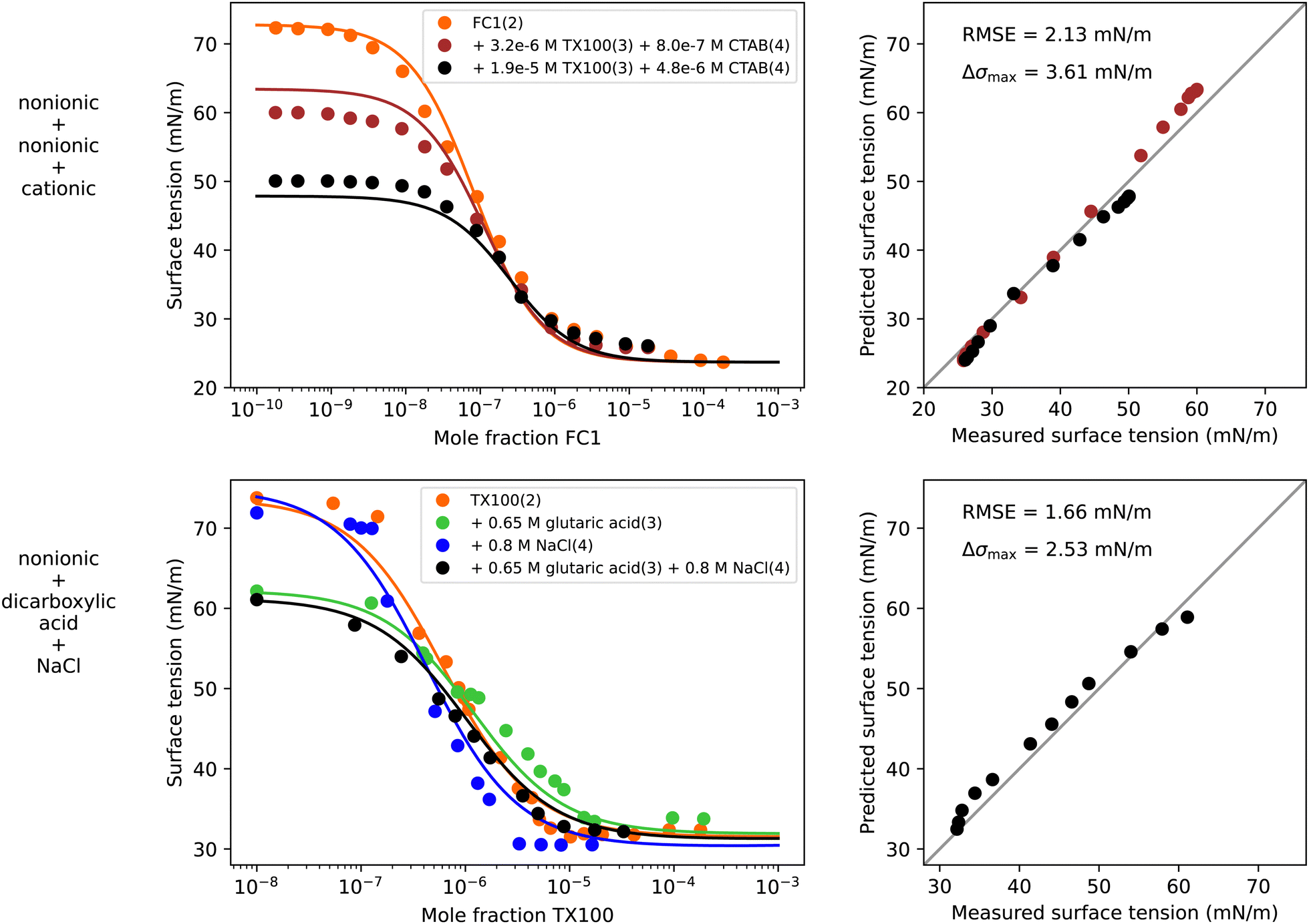 | ||
| Fig. 8 Surface tension of two quaternary systems. Left panels show experimental data (symbols) and model results (solid lines) from eqn (6), (9), (10), (12), and (13) for the quaternary system and ternary and binary subsystems. Right panels show the error in predicted surface tension for all quaternary data points. First row: Water (1) + FC1 (2) + TX100 (3) + CTAB (4), T = 20 °C, data from Jańczuk et al.66 Second row: Water (1) + TX100 (2) + glutaric acid (3) + NaCl (4), T = 24 °C, data from this study. | ||
To test if the model can be applied to an atmospherically relevant system containing water, a surfactant, an organic substance and a salt, the surface tension of TX100 in an aqueous solution of 0.65 M glutaric acid and 0.8 M NaCl in water was measured by pendant drop tensiometry at 24 °C. The experimental data was obtained from Manuella El Haber by personal communication and the measurement procedure was identical to that described in El Haber et al.40 The experimental data is shown in Fig. 8 in the lower left panel as black circles. To model this quaternary systems, the same σi values and binary water–solute separation factors S1i were taken as for the systems water–TX100–NaCl and water–TX100–glutaric acid modelled previously (Fig. S9 and S10 in ESI,† respectively). Parameters ASO24, BSO24, and BSO34 for the salting-out of glutaric acid and TX100 by NaCl were taken from the previously modelled systems water–glutaric acid–NaCl and water–TX100–NaCl (Fig. 5 and 6, respectively). Water-free separation factors Sij were all set to unity. Based on these parameters, which are summarized in Table 3 under “q2”, the predicted quaternary surface tension resulted in a very good agreement with the experimental data with a maximum deviation of only 2.53 mN m−1.
Given the simplicity of the model approach, it might be surprising how well the quaternary systems were predicted using binary and ternary solution data only. Yet, as the Eberhart model can be derived from the Chunxi model,31 it has a strong thermodynamic background. Moreover, the physical and chemical properties of multi-component mixtures usually stem from binary and ternary interactions between the system components. In the absence of binary interactions between the solute molecules, the ternary system can indeed be predicted from the respective binary systems. While binary molecular interactions are of high importance to determine bulk properties, ternary or higher-order molecular interactions contribute relatively little to physical properties of mixtures and are often truncated in theoretical descriptions (e.g., Pitzer activity coefficients, virial coefficients, etc.). The thermodynamic background of the modelling approach and the absence of higher-order interactions between solutes in the quaternary systems therefore allowed us to predict the quaternary systems and should also result in successful predictions of more complex mixtures.
5 Summary and conclusions
In this study, a multi-component model based on the Eberhart equation is presented and tested on experimental surface tension data of 22 ternary systems and two quaternary systems with solutes covering inorganic salts, organic substances and amphiphilic surfactants. A total of 1842 data points of ternary solutions were modelled with an overall RMSE of 3.09 mN m−1.To model the surface tension of ternary mixtures, the model requires binary surface tension data to fit the separation factors Sij. If the system behaves ideally, the ternary surface tensions can be predicted with eqn (6) knowing only the binary parameters. If the separation factor of a binary system is missing, the ternary system can be modelled by fitting the missing parameter to ternary surface tension data. In aqueous systems, ternary data are often only available for dilute aqueous solutions. As a result, the separation factor between the solutes is unconstrained, in which case we set it to 1. In this case, the predicted surface tension values can become unreliable outside the fitted data range.
To accurately model systems that exhibit non-ideal behavior, additional parameters Aij and Bij were introduced that need to be fitted to ternary data. Two different cases were distinguished: in systems with salts or other ionic substances, non-ideality is driven by salting-out, which is modelled with eqn (9) and (10). Non-ideality related to the formation of mixed micelles is modelled with eqn (12) and (13). All parameters used to model the ternary systems shown in this study are summarized in Table 1, as well as the RMSE and maximum error.
The model showed excellent performance for ternary water–organic–organic systems (RMSEs < 1.14 mN m−1). Water–surfactant–surfactant systems including strongly non-ideal catanionic and zwitterionic surfactant mixtures could be modelled with good accuracy (RMSEs < 3.82 mN m−1), when fitting non-ideality factors. Salting-out was found to be important for water–organic–salt systems, which could be modelled well in the dilute concentration range where data was available (RMSEs < 3.19 mN m−1). Besides bulk non-ideality induced by salting-out, water–surfactant–salt systems also showed surface synergistic behaviour, both of which could be captured by the model and RMSEs remained below 3.83 mN m−1. The model could also reproduce the surface tension data of five water–surfactant–organic systems with RMSEs ranging from 2.33 mN m−1 to 8.57 mN m−1, and it was found that systems containing oxalic acid show salting-out driven non-ideal behaviour that depends on the dilution with water. To conclude, the model proved to be able to describe aqueous solutions containing salts, organics, and amphiphilic surfactants and their ternary mixtures, which, to our knowledge, has not been achieved by any previous model.
One of the strengths of the presented model is that it can predict quaternary surface tension data without additional fit parameters, given that all parameters of the ternary subsystems are known. This was illustrated for two different systems with very good performance (see Fig. 8). The fit parameters, the RMSE and the maximum error of these systems are shown in Table 3. The surface tension of a quaternary mixture containing a surfactant, a water-soluble organic substance, a salt and water was well predicted, which has not been achieved before. This system can therefore be used to estimate the surface tension of atmospheric aerosol particles, that contain water, salts, organics and surfactants.
Since binary water–solute surface tension data is broadly available in the literature but water-free binary data and ternary data is more scarce, the model could be further improved if the water-free separation factor and the non-ideality factors could be estimated based on the molecular structures of the solutes. As could be seen from the systems containing salts, the salting-out related bulk non-ideality factor BSO23 seems to depend on the ionic strength of the bulk phase as well as on the hydrophobicity of the organic molecule. In order to explore the relationship between these factors and the solute types, clearly more experimental surface tension data is required covering a broader variety of mixtures and a larger concentration range, including high solute concentrations.
Further studies should focus on measuring more ternary systems, which might allow to get a better understanding of the physical and chemical processes in such complex mixtures. In particular, measurements of salt–alcohol–water systems, surfactant–alcohol–water systems and measurements at high solute concentrations would be most helpful. Furthermore, temperature dependence could be analyzed, and the predictive capabilities of the model could be investigated further, e.g. by correlating non-ideality factors with solute properties.
Data availability
Data for this paper, including the experimental surface tension data and fit parameters are available at https://doi.org/10.5281/zenodo.10550607 and a python code of the Eberhart model at https://doi.org/10.5281/zenodo.10889512.Author contributions
J. K. conducted the data curation, the formal analysis, the visualizations, and wrote the original draft. C. M. acquired the funding and administrated the project and supervised J. K. together with N. S. All authors contributed to conceptualization, methodology and writing (review & editing), and all authors have approved the final version of the paper.Conflicts of interest
There are no conflicts to declare.Acknowledgements
This research has been funded by the Swiss National Science Foundation (SNF; grant no. 200021L_197149) as part of the ORACLE project. This material is also based upon work supported by the Humphreys Engineer Center Support Activity under contract no. W912HQ20C0041, corresponding to US Department of Defense Strategic Environmental Research and Development Program (SERDP) project WP19-1407. We thank Manuella El Haber for measuring the quaternary surface tension shown in Fig. 8 and we acknowledge fruitful discussions with Manuella El Haber, Barbara Noziere, Corinne Ferronato, and Thomas Peter. We also thank Mohsin Qazi for providing the experimental surface tension data of Qazi et al.58 in tabular form. Lastly, we thank Ulrike Lohmann for providing infrastructure for this project.Notes and references
- M. Ali, B. Pan, N. Yekeen, S. Al-Anssari, A. Al-Anazi, A. Keshavarz, S. Iglauer and H. Hoteit, Int. J. Hydrogen Energy, 2022, 47, 14104–14120 CrossRef CAS.
- R. Ananth, A. W. Snow, K. M. Hinnant, S. L. Giles and J. P. Farley, Colloids Surf., A, 2019, 579, 123686 CrossRef.
- H. Köhler, Trans. Faraday Soc., 1936, 32, 1152–1161 RSC.
- C. Marcolli, B. Luo and T. Peter, J. Phys. Chem. A, 2004, 108, 2216–2224 CrossRef CAS.
- U. Lohmann, F. Lüönd and F. Mahrt, An Introduction to Clouds: From the Microscale to Climate, Cambridge University Press, 2016 Search PubMed.
- B. R. Bzdek, J. P. Reid, J. Malila and N. L. Prisle, Proc. Natl. Acad. Sci. U. S. A., 2020, 117, 8335–8343 CrossRef CAS PubMed.
- R. Sorjamaa, B. Svenningsson, T. Raatikainen, S. Henning, M. Bilde and A. Laaksonen, Atmos. Chem. Phys., 2004, 4, 2107–2117 CrossRef CAS.
- J. Malila and N. L. Prisle, J. Adv. Model. Earth Syst., 2018, 10, 3233–3251 CrossRef CAS PubMed.
- S. Vepsäläinen, S. M. Calderón and N. L. Prisle, EGUsphere, 2023, vol. 2023, pp. 1–23.
- J. L. Jimenez, M. R. Canagaratna, N. M. Donahue, A. S. H. Prevot, Q. Zhang, J. H. Kroll, P. F. DeCarlo, J. D. Allan, H. Coe, N. L. Ng, A. C. Aiken, K. S. Docherty, I. M. Ulbrich, A. P. Grieshop, A. L. Robinson, J. Duplissy, J. D. Smith, K. R. Wilson, V. A. Lanz, C. Hueglin, Y. L. Sun, J. Tian, A. Laaksonen, T. Raatikainen, J. Rautiainen, P. Vaattovaara, M. Ehn, M. Kulmala, J. M. Tomlinson, D. R. Collins, M. J. Cubison, E. J. Dunlea, J. A. Huffman, T. B. Onasch, M. R. Alfarra, P. I. Williams, K. Bower, Y. Kondo, J. Schneider, F. Drewnick, S. Borrmann, S. Weimer, K. Demerjian, D. Salcedo, L. Cottrell, R. Griffin, A. Takami, T. Miyoshi, S. Hatakeyama, A. Shimono, J. Y. Sun, Y. M. Zhang, K. Dzepina, J. R. Kimmel, D. Sueper, J. T. Jayne, S. C. Herndon, A. M. Trimborn, L. R. Williams, E. C. Wood, A. M. Middlebrook, C. E. Kolb, U. Baltensperger and D. R. Worsnop, Science, 2009, 326, 1525–1529 CrossRef CAS PubMed.
- R. E. Cochran, O. Laskina, T. Jayarathne, A. Laskin, J. Laskin, P. Lin, C. Sultana, C. Lee, K. A. Moore, C. D. Cappa, T. H. Bertram, K. A. Prather, V. H. Grassian and E. A. Stone, Environ. Sci. Technol., 2016, 50, 2477–2486 CrossRef CAS PubMed.
- S. Frka, J. Dautović, Z. Kozarac, B. Ćosović, A. Hoffer and G. Kiss, Tellus B, 2012, 64, 18490 CrossRef CAS.
- V. Gérard, B. Noziere, L. Fine, C. Ferronato, D. K. Singh, A. A. Frossard, R. C. Cohen, E. Asmi, H. Lihavainen, N. Kivekäs, M. Aurela, D. Brus, S. Frka and A. Cvitešić Kušan, Environ. Sci. Technol., 2019, 53, 12379–12388 CrossRef PubMed.
- M. T. Latif and P. Brimblecombe, Environ. Sci. Technol., 2004, 38, 6501–6506 CrossRef CAS PubMed.
- H. Tervahattu, J. Juhanoja, V. Vaida, A. F. Tuck, J. V. Niemi, K. Kupiainen, M. Kulmala and H. Vehkamäki, J. Geophys. Res.: Atmos., 2005, 110, D06207 CrossRef.
- J. G. Eberhart, J. Phys. Chem., 1966, 70, 1183–1186 CrossRef CAS.
- K. A. Connors and J. L. Wright, Anal. Chem., 1989, 61, 194–198 CrossRef CAS.
- J. Kleinheins, N. Shardt, M. El Haber, C. Ferronato, B. Nozière, T. Peter and C. Marcolli, Phys. Chem. Chem. Phys., 2023, 25, 11055–11074 RSC.
- J. A. V. Butler, Proc. R. Soc. London, Ser. A, 1932, 135, 348–375 CAS.
- B. E. Poling, J. M. Prausnitz and J. P. O’Connell, Properties of Gases and Liquids, McGraw-Hill Education, New York, 5th edn, 2001, ch. 12 Search PubMed.
- Z. Li and B. C.-Y. Lu, Chem. Eng. Sci., 2001, 56, 2879–2888 CrossRef CAS.
- A. S. Wexler and C. S. Dutcher, J. Phys. Chem. Lett., 2013, 4, 1723–1726 CrossRef CAS PubMed.
- H. Boyer, A. Wexler and C. Dutcher, J. Phys. Chem. Lett., 2015, 6, 3384–3389 CrossRef CAS PubMed.
- H. C. Boyer and C. S. Dutcher, J. Phys. Chem. A, 2017, 121, 4733–4742 CrossRef CAS PubMed.
- B. von Szyszkowski, Z. Phys. Chem., 1908, 64U, 385–414 CrossRef.
- I. Langmuir, J. Am. Chem. Soc., 1917, 39, 1848–1906 CrossRef CAS.
- S. Henning, T. Rosenørn, B. D’Anna, A. A. Gola, B. Svenningsson and M. Bilde, Atmos. Chem. Phys., 2005, 5, 575–582 CrossRef CAS.
- J. J. Lin, J. Malila and N. L. Prisle, Environ. Sci.: Processes Impacts, 2018, 20, 1611–1629 RSC.
- A. Z. Mazurek, S. J. Pogorzelski and A. D. Kogut, Atmos. Environ., 2006, 40, 4076–4087 CrossRef CAS.
- A. N. Schwier, G. A. Viglione, Z. Li and V. Faye McNeill, Atmos. Chem. Phys., 2013, 13, 10721–10732 CrossRef.
- L. Chunxi, W. Wenchuan and W. Zihao, Fluid Phase Equilib., 2000, 175, 185–196 CrossRef CAS.
- N. Shardt, Y. Wang, Z. Jin and J. A. Elliott, Chem. Eng. Sci., 2021, 230, 116095 CrossRef CAS.
- N. Shardt and J. A. W. Elliott, Langmuir, 2017, 33, 11077–11085 CrossRef CAS PubMed.
- R. Tahery, H. Modarress and J. Satherley, Chem. Eng. Sci., 2005, 60, 4935–4952 CrossRef CAS.
- J. Shereshefsky, J. Colloid Interface Sci., 1967, 24, 317–322 CrossRef CAS.
- H. G. Hauthal, P. Jürges, L. Möhle and U. Ohlerich, J. Surfactants Deterg., 1999, 2, 175–180 CrossRef CAS.
- M. Agneta, L. Zhaomin, Z. Chao and G. Gerald, J. Pet. Sci. Eng., 2019, 175, 489–494 CrossRef CAS.
- X. Y. Hua and M. J. Rosen, J. Colloid Interface Sci., 1982, 90, 212–219 CrossRef CAS.
- V. Fainerman, R. Miller and E. Aksenenko, Adv. Colloid Interface Sci., 2002, 96, 339–359 CrossRef CAS PubMed.
- M. El Haber, C. Ferronato, A. Giroir-Fendler, L. Fine and B. Nozière, Sci. Rep., 2023, 13, 20672 CrossRef CAS PubMed.
- G. Tyagi, D. Seddon, S. Khodaparast, W. N. Sharratt, E. S. Robles and J. T. Cabral, Colloids Surf., A, 2021, 618, 126414 CrossRef CAS.
- M. Bielawska, A. Chodzińska, B. Jańczuk and A. Zdziennicka, Colloids Surf., A, 2013, 424, 81–88 CrossRef CAS.
- W. Wagner and H.-J. Kretzschmar, International Steam Tables: Properties of Water and Steam Based on the Industrial Formulation IAPWS-IF97, Springer Berlin Heidelberg, Berlin, Heidelberg, 2008, pp. 7–150 Search PubMed.
- G. J. Janz, J. Phys. Chem. Ref. Data, 1980, 9, 791–830 CrossRef CAS.
- G. J. Janz, J. Phys. Chem. Ref. Data, 1988, 17(Suppl. 2), 1–309 Search PubMed.
- C. S. Dutcher, A. S. Wexler and S. L. Clegg, J. Phys. Chem. A, 2010, 114, 12216–12230 CrossRef CAS PubMed.
- P. Virtanen, R. Gommers, T. E. Oliphant, M. Haberland, T. Reddy, D. Cournapeau, E. Burovski, P. Peterson, W. Weckesser, J. Bright, S. J. van der Walt, M. Brett, J. Wilson, K. J. Millman, N. Mayorov, A. R. J. Nelson, E. Jones, R. Kern, E. Larson, C. J. Carey, İ. Polat, Y. Feng, E. W. Moore, J. VanderPlas, D. Laxalde, J. Perktold, R. Cimrman, I. Henriksen, E. A. Quintero, C. R. Harris, A. M. Archibald, A. H. Ribeiro, F. Pedregosa, P. van Mulbregt and SciPy 1.0 Contributors, Nat. Methods, 2020, 17, 261–272 CrossRef CAS PubMed.
- A. Rafati, A. Bagheri and M. Najafi, J. Chem. Thermodyn., 2011, 43, 248–254 CrossRef CAS.
- B. Santos, A. Ferreira and I. Fonseca, Fluid Phase Equilib., 2003, 208, 1–21 CrossRef CAS.
- L. Y. Zakharova, F. G. Valeeva, A. R. Ibragimova, V. M. Zakharov, L. A. Kudryavtseva, Y. G. Elistratova, A. R. Mustafina, A. I. Konovalov, S. N. Shtykov and I. V. Bogomolova, Colloid J., 2007, 69, 718–725 CrossRef CAS.
- K. Szymczyk and B. Jańczuk, Colloids Surf., A, 2007, 293, 39–50 CrossRef CAS.
- R. Miles, M. Glerum, H. Boyer, J. Walker, C. Dutcher and B. Bzdek, J. Phys. Chem. A, 2019, 123, 3021–3029 CrossRef CAS PubMed.
- J. Vanhanen, A.-P. Hyvärinen, T. Anttila, T. Raatikainen, Y. Viisanen and H. Lihavainen, Atmos. Chem. Phys., 2008, 8, 4595–4604 CrossRef CAS.
- A.-P. Hyvärinen, T. Raatikainen, A. Laaksonen, Y. Viisanen and H. Lihavainen, Geophys. Res. Lett., 2005, 32, L16806 CrossRef.
- A. M. Booth, D. O. Topping, G. McFiggans and C. J. Percival, Phys. Chem. Chem. Phys., 2009, 11, 8021–8028 RSC.
- O. Ozdemir, S. I. Karakashev, A. V. Nguyen and J. D. Miller, Miner. Eng., 2009, 22, 263–271 CrossRef CAS.
- H. Nakahara, O. Shibata and Y. Moroi, J. Phys. Chem. B, 2011, 115, 9077–9086 CrossRef CAS PubMed.
- M. J. Qazi, S. J. Schlegel, E. H. Backus, M. Bonn, D. Bonn and N. Shahidzadeh, Langmuir, 2020, 36, 7956–7964 CrossRef CAS PubMed.
- G. Para, E. Jarek and P. Warszynski, Colloids Surf., A, 2005, 261, 65–73 CrossRef CAS.
- P. Basařová, T. Váchová and L. Bartovská, Colloids Surf., A, 2016, 489, 200–206 CrossRef.
- S. Syeda, A. Afacan and K. Chuang, Chem. Eng. Res. Des., 2004, 82, 762–769 CrossRef CAS.
- E. Rio, W. Drenckhan, A. Salonen and D. Langevin, Adv. Colloid Interface Sci., 2014, 205, 74–86 CrossRef CAS PubMed.
- E. W. Kaler, A. K. Murthy, B. E. Rodriguez and J. A. N. Zasadzinski, Science, 1989, 245, 1371–1374 CrossRef CAS PubMed.
- T. H. Bertram, R. E. Cochran, V. H. Grassian and E. A. Stone, Chem. Soc. Rev., 2018, 47, 2374–2400 RSC.
- V. Gérard, B. Nozière, C. Baduel, L. Fine, A. A. Frossard and R. C. Cohen, Environ. Sci. Technol., 2016, 50, 2974–2982 CrossRef PubMed.
- B. Jańczuk, K. Szymczyk and A. Zdziennicka, Molecules, 2021, 26, 4313 CrossRef PubMed.
Footnote |
| † Electronic supplementary information (ESI) available. See DOI: https://doi.org/10.1039/d4cp00678j |
| This journal is © the Owner Societies 2024 |