
Emerging investigator series: moving beyond resilience by considering antifragility in potable water systems
Joseph E.
Goodwill
 *a,
Patrick
Ray
b,
Destenie
Nock
c and
Christopher M.
Miller
d
*a,
Patrick
Ray
b,
Destenie
Nock
c and
Christopher M.
Miller
d
aDept. of Civil & Environmental Engineering, University of Rhode Island, Kingston, RI, USA. E-mail: goodwill@uri.edu
bDept. of Chemical & Environmental Engineering, University of Cincinnati, Cincinnati, OH, USA
cDept. of Civil & Environmental Engineering, and, Dept. of Engineering & Public Policy, Carnegie Mellon University, Pittsburgh, PA, USA
dDept. of Civil Engineering, University of Akron, Akron, OH, USA
First published on 11th November 2021
Abstract
It is inherently difficult to plan water systems for a future that is non-predictive. This paper introduces a novel perspective for the design and operation of potable water systems under increasing water quality volatility (e.g., a relatively rapid and unpredicted deviation from baseline water quality). Increased water quality volatility and deep uncertainty stress water systems, confound design decisions, and increase the risk of decreased water system performance. Recent emphasis on resilience in drinking water treatment has partly addressed this issue, but still establishes an adversarial relationship with change. An antifragile system benefits from volatile change. By incorporating antifragility, water systems may move beyond resilience and improve performance with extreme events and other changes, rather than survive, or fail and quickly recover. Using examples of algal blooms, wildfires, and the COVID-19 pandemic, this work illustrates fragility, resilience, and antifragility within physicochemical process design including clarification, adsorption and disinfection. Methods for increasing antifragility, both individual process options and new system design tools, are discussed. Novel physicochemical processes with antifragile characteristics include ferrate preoxidation and magnetic iron (nano)particles. New design tools that allow for systematic evaluation of antifragile opportunities include artificial neural networks and virtual jar or pilot “stress testing”. Incorporating antifragile characteristics represents a trade-off with capital and/or operating cost. We present a real options analysis approach to considering costs in the context of antifragile design decisions. Adopting this antifragile perspective will help ensure water system improved performance during extreme events and a general increase in volatility.
Water impactRaw water quality volatility driven by extreme events presents a grand challenge to potable water systems. This work describes a new perspective of antifragility that allows water systems to thrive despite an uncertain future. Individual processes that have antifragile characteristics are introduced and discussed, as well as new tools for water system design that allow for considerations of antifragility. Incorporation of the antifragile paradigm developed here will enable a shift towards more sustainable water systems less reliant on stationarity and prediction of future conditions. |
Introduction
Engineered systems that produce and distribute potable water are critically important to public health. Potable water systems (PWS) have led to dramatic decreases in waterborne diseases,1 at a low cost relative to public value.2 PWS face challenges, especially related to uncertainty and volatility. For example, source water quality and quantity may be affected by extreme events and phenomena such as chemical spills,3 harmful algal blooms,4 hurricanes,5,6 and wildfires.7,8 Some water changes may be driven by climate change, although predictive modeling of this relationship is difficult at the watershed spatial scale.9 PWS may also be impacted by complex socioeconomic processes such as economic globalism, leading to population loss (e.g., “shrinking cities”) and corresponding water age increases,10 and possible water quality problems.11 These processes generally contribute to volatility, uncertainty, complexity and ambiguity (VUCA). This combination of stressors comprise a “deep uncertainty” that confounds the design and planning of water systems.12Water treatment processes have historically been designed using a deterministic approach.13,14 In the deterministic approach, modeling efforts intended to assist in process optimization have tended to assume that the influent water quality conditions, water demands, and model parameters are fixed and known. This assumption has proven dubious as new types of contamination (e.g., perfluorinated compounds, pharmaceuticals) have emerged, and surface water quality variability has increased.15 More recently, researchers have advocated for the incorporation of variability and uncertainty of source water quality in water treatment plant design and operation, but have continued an optimality paradigm with regard to water treatment plant effluent.16–18 The deterministic approach remains the current dominant paradigm in water treatment process design and operation, and is enshrined in published process selection guidance (see ref. 13 as an example).
An example consequence of the optimality paradigm is the exclusion of clarification from some PWS treatment trains (e.g., direct filtration). Given source water of sufficient average historical quality (i.e., the constraint), water treatment plants have been designed to minimize lifetime construction and operation costs (i.e., the objective). This model has been generally successful; however, a loss of (perceived) stationarity undermines the optimality paradigm, with accelerating rates of change and more numerous extreme events projected.19,20 The optimality paradigm is highly constrained and fragile to baseline water quality deviations, and is not appropriate for cases of deep uncertainty, as is now faced by water treatment plant operators and planners.21 Also, it is highly dependent upon the quality of simulation models representing the water treatment system; unfortunately, we know the quality of the available models to be relatively poor.16,22 Further, common physical models such as jar testing and pilot testing informing PWS decision making provide no information about future water conditions or performance. Elements of the outcome for the optimality paradigm approach therefore contain stochastic elements, making the outcomes also inherently stochastic.23 An alternative decision making analytical approach is needed.
PWS decision making has been shifting to the incorporation of robustness, resilience, and adaptation.24,25 In the United States, The National Infrastructure Advisory Council (NIAC) defined resilient infrastructure as able to anticipate, adsorb or adapt to, and/or recover from a disruptive event, and encourages planners and designers to aim for resilience in designs for infrastructure.26,27 Similarly, America's Water Infrastructure Act requires most PWS to conduct a risk and resilience assessment by the end of 2021.28 Common design changes to increase resilience in PWS include additional redundancy and capacity.21 These changes have decreased risk of water system failure; however, this approach is still somewhat dependent on prediction of future events and limiting service disruptions, not improving service in the face of volatility. If volatility is increasing then the adversarial relationship with it inherent in the resilience paradigm is unsustainable.
This paper describes a novel perspective for achieving an antifragility paradigm in PWS design and operation, including cost trade-offs. The antifragile concept was popularized in the financial domain,29 but has been applied in other fields, such as computer science and transportation planning,30 as an approach to risk. In the antifragility paradigm a system benefits from volatility, rather than being harmed by it.29 In this way, antifragility extends resilience/robustness frameworks. Robust infrastructure resists failure, often through the adoption of conservative designs that include excess capacity. Resilient infrastructure systems fail, but not catastrophically, and recover somewhat quickly. The key benefit of antifragility is that performance actually improves in volatile periods. It also is less reliant on prediction of the future. The overarching objective of this paper is to introduce the antifragility paradigm across domains into PWS, and frame raw water quality volatility and extreme (e.g., “black swan”) events in the water supply sector that may be better managed with via antifragility. We also include examples of novel physicochemical processes that have antifragile characteristics and summarize new design tools that allow for systematic consideration of antifragility in the field of water treatment.
Black swan events
We define volatility as the (relatively) rapid and unpredicted deviation from a baseline (i.e., “normal”). Specific instances of volatility can be labeled as a black swan event. The term black swan event (BSE) was also popularized in the financial domain, and is generally taken to mean a low probability event, with casual opacity, that is difficult to predict.31 Quantitatively, this can be summarized as an event more than a few standard deviations away from the mean of prior data; an outlier. Casual opacity may also be a characteristic, leading to uncertainty in what initiated the low probability event. These characteristics of BSEs ultimately make them impossible to predict with confidence. Often, insufficient data (e.g., sample size) make the nature of the event probability unknowable, and leave it unclear if a system follows as Gaussian distribution, or another distribution with skewness (e.g., gamma family), or fat tails (e.g., Cauchy).32,33Here, we take this concept cross domain into the environmental engineering context, focused on PWS. Water systems are exposed to BSEs. Examples receiving recent attention include lake recovery,34 and forest fires.35 Both of these BSE examples have impacts to source water quality that are an extreme departure from historical averages.36 Also, the cause of these events is difficult to determine. Lake recovery is a relatively rapid increase in organic productivity or “browning” of a surface water driven by a complex combination of nutrient loadings, warming air temperatures (e.g., climate change),37 and decreases in sulfur deposition from upwind sources.38 In Atlantic Canada, decreases in sulfur deposition followed the amendments of the US Clean Air Act, illustrating the causal opacity and deep complexity of secondary effects in PWS design. Similarly, large-scale forest fires may form via anthropogenic or natural phenomena and are likely exasperated by climate change, invasive insect activity, and forest management policies. The total annual acreage burned by wildfires in the US more than tripled from 1983 to 2016.35 Wildfires are known to cause changes in watersheds that impact water quality including increases in turbidity, nitrate, phosphate, and disinfection byproduct precursors that may persist for several years postfire.39,40
The problem caused by exposure to a BSE by a PWS often presents in difficulty achieving treatment goals following dramatic changes in raw water quality. These source water shifts may exceed the design capacity of any physicochemical process that comprises a given drinking water treatment plant. Two examples of this situation are presented in Fig. 1, which includes raw water organics (color or total organic carbon) and turbidity for two different source waters: (1) A reservoir before and after lake recovery–Pockwock Lake,34 and (2) a river draining an alpine forest before and after a major wildfire–Poudre River.8Fig. 1 also includes regions of recommended clarification design from Valade et al., 2009 based primarily on American Water Works Association survey of utilities.41 Gaussian distributions were assumed for both organics and turbidity.
 | ||
| Fig. 1 Results of 365 statistical resamplings of distributions based on average raw water quality from Pockwock Lake (PL) in 1999 (gray circle) and 2015 (green circle) and from the Poudre River (PR) from 2008–2011 (gray triangle) and 2013 (red triangle). PL plots are color vs. turbidity; PR plots are TOC vs. turbidity. Regions of typical particle removal designs include direct filtration (DF), dissolved air flotation (DAF) and conventional sedimentation from Valade et al., 2009. Relative scaling of color and TOC within design regions also taken from Valade et al., 2009.41 Raw water quality statistical information from PL and PR taken from Anderson et al., 2017 (ref. 34) and Hohner et al., 2016 (ref. 8), respectively. | ||
Fig. 1 demonstrates that shifts in raw water quality from BSEs can change the optimal design of a drinking water treatment plant (DWTP). Optimal clarification design guidance is summarized in Valade et al., 2009 (ref. 41) and Gregory and Edzwald, 2011 (see Table 9.9 in that work).42 Utilizing raw quality data from Pockwock Lake (PL) in 1999, a designer using the optimality paradigm may recommended direct filtration (DF) to save costs by excluding any clarification step.13 Similarly, an optimality-based designer presented with PR data in 2011 may consider DAF clarification in an attempt to save space and capital costs. DAF systems can be operated at a loading rate 10–20 times greater than conventional gravity sedimentation.43 However, a DAF design may struggle post wildfire, as resampled turbidities are significantly greater than the pre-fire condition. The J.D. Kline Water Supply Plant (JDKWSP) utilizing PL was designed as a direct filtration facility. This design was optimal at the time; in 1999 water quality was within the DF design region in 92% of simulations. However, JDKWSP is now straining to meet treatment goals due to lake recovery as the raw water typically exceeds the recommended limits for a DF facility. Fig. 1 shows raw water quality exceeding the recommended color limit of the DF design region 58% of simulations. As a DF facility, few mitigative options are available. For the first time in 35 years, the JDKWSP recently increased its coagulation (alum) dose by 50%,44 which may have negative higher-order effects associated with increased levels of effluent aluminum and subsequent changes on distribution system corrosion.45 Recent pilot-scale research at JDKWSP has also examined cationic polymers, and larger filter media. Neither mitigation approach was completely successful and now physical plant upgrades are being considered. To what conditions the plant might be optimized in the future remains unclear.44 The situation at JDKWSP exemplifies difficulties presented by BSEs to drinking water systems. The Fort Collins Water Treatment Facility, which treats surface water from the Poudre River watershed, rapidly constructed a presedimentation basin as a response to observed turbidity volatility following a major wildfire.39
Fragile, resilient, and antifragile
Future BSEs and general volatility are difficult to predict, so it is more profitable to define a system based on relative impact from stress. This approach has again been popularized in financial markets through stress testing.46 The three primary relationships to stress may be described as fragile, resilient, and antifragile. A fragile system has severe negative outcomes from volatility, a resilient system has minor negative outcomes from volatility with relatively quick recovery, while an antifragile system has positive outcomes from volatility. Mathematical expressions of all three terms exist;47 however, model-free and probability-free heuristics can also be used to assess fragility, resilience, and antifragility based on a convex relationship to volatility.48 Fragile and antifragile systems have negative and positive convex relationships with volatility, respectively, while resilience has a linear relationship with volatility. Here, we apply a heuristic approach to identifying fragile, resilient, and antifragile PWS based on convexity using data from full-scale DWTPs,Fragility, resilience/robustness, and antifragility are currently present in contemporary full-scale DWTPs. Examples of each include the Lake Major Water Supply Plant (#1 fragile); the Providence Water System (#2 resilient) and for two surface water sourced DWTPs in New England (#3 antifragile). The Lake Major Water Supply Plant and the Providence Water System are also both surface water sourced systems.
Fragile
The Lake Major Water Supply Plant (LMWSP) was commissioned in 1999 as a conventional sedimentation facility treating a high-quality source, Lake Major (LM). The LMWSP serves the same general population as JDKWSP, Halifax, Canada. Similar to Pockwock Lake, Lake Major has also experienced lake recovery since commission, resulting in an increase in raw water algal organics as noted by color measurements, shown in Fig. 2. Algae challenge conventional sedimentation-based DWTPs in two ways: the algal organic matter exhibits an increased coagulant demand, and algal particles settle quite slowly due to specific gravities ≤1.49 The LMWSP has few mitigative operational controls, and has increased alum dosing in response to increased water color. Fig. 2 shows an exponential (e.g., convex) relationship between raw water color and required alum dose. This indicates accelerating problematic fragility to further increases in water color. For example, an increase in color 5 units from 25 to 30 resulted in an alum increase of 20%, while the same 5 unit increase from 42 to 47 resulted in an alum increase of almost 50%. Results indicate accelerating problems and risk of system failure with further increase in raw water color, even if only incremental. Significant increases in alum dose carry the potential for numerous negative second-order effects, such as increased chemical costs, decreased filter run times, increased solids handling stress, and increased distribution system corrosion.44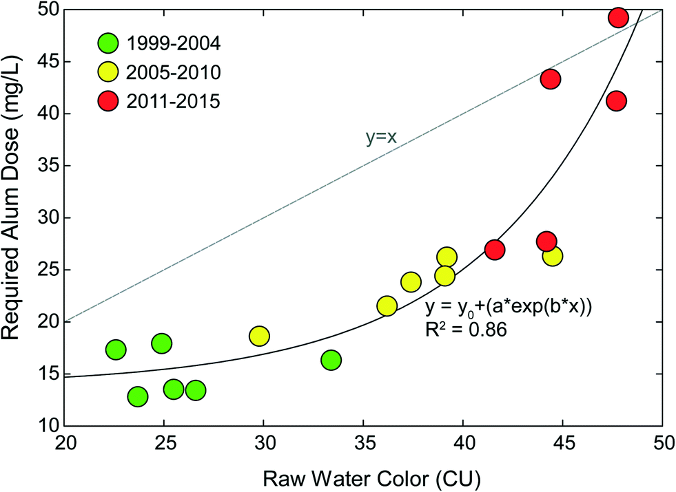 | ||
| Fig. 2 Yearly mean raw water color and corresponding coagulant dose at the Lake Major Water Supply Plant from 1999 through 2015. Data from Anderson et al., 2017.34 Note the non-linear (e.g., convex) relationship between color and required alum dose demonstrating fragility. Incremental increases in color above 40 CU led to exponential increases in alum dose. | ||
Resilient
The Providence Water Supply Board (PW) operates the largest conventional DWTP in the Northeast USA. PW has a history of providing safe water service but recent, occasional issues with disinfection byproducts (DBPs), especially total trihalomethanes (TTHMs), have occurred including an maximum contaminant limit (MCL) violation in 2018.50 One particular DBP monitoring site tends to control MCL compliance; a large elevated storage tank in a remote part of the system. PW had recently installed a THM-stripping aeration system in the tank, just prior to the BSE of the COVID-19 pandemic. Changes in commuting and other behavioral patterns led to changes in water usage within the service area's urban core. Water ages increased, and thus the THM formation also increased. Trihalomethane formation potential (THMFP) is a function of several drivers including precursory organic carbon, residual chlorine concentrations, temperature, and water age.51 Methods exists for estimating site-specific THMFP based on dissolved organic carbon (DOC), UV absorbance, and other water quality parameters.52,53 Using an approach outlined in ref. 52 the THMFP for PW effluent is estimated to range from 100 to 150 μg L−1, significantly greater than the 80 μg L−1 MCL for TTHMs.The increase in water age created stress on the PW system to meet the MCL. Results in Fig. 3 show rapidly increasing THMs in March 2020, with one sample above 70 μg L−1. Aeration was initiated in April. Aeration within the storage tank was effective at decreasing THMs in the delivered water and THM values decreased to well below the MCL. The impact of aeration is also noted in July 2020 when aeration was temporarily ceased. The use of aeration represents a form of resilience for PW. Given serious stress from the COVID-19 BSE (increase in THMs), the system was able to mitigate the damage, and continue to meet treatment goals, after a temporary increase in delivered water THMs. There is a linear (non-convex) relationship between volatility and THMs as the presence of aerators provides a switch-on recovery option that can be utilized as needed. This THM mitigative approach generally meets the NIAC definition of resilience: “the ability to reduce the magnitude and/or duration of disruptive events through the ability to anticipate, absorb, adapt to, and/or rapidly recover”.27
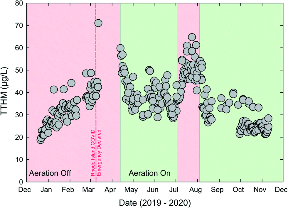 | ||
| Fig. 3 Total trihalomethane (TTHM) concentrations measured as at an elevated storage tank within a problematic water age area of the Providence Water (PW) system from December 2019 through November 2020. Shaded regions represent periods when an aeration system inside the elevated storage tank was in operation. PW THM formation potential estimated to be 100 to 140 μg L−1. | ||
Resilience may also be considered at the system level. In general, the more diverse a system is (e.g., multiple sources and/or production) the more resilient it is to a particular disruption; while a highly centralized system is more fragile.29 The relationship between centralization and fragility has been commonly explored in a financial context (e.g., “a diversified portfolio”), however, recent work has advocated for water supply systems to not be reliant upon a single source of water.54 A comparison between the water systems of Rhode Island, USA and Singapore demonstrates this difference. The PW system, consisting of one conventional water treatment plant, provides water to approximately two-thirds of Rhode Island residents, as many communities outside of Providence are wholesale customers through interconnections. While this is efficient, it also fragile as any BSE or other disruption at the PW treatment plant would impact potable water access to much of the state. Contrastingly, the Singapore Four National Taps approach includes water imports, direct potable reuse (i.e., NEWater), desalination, and runoff from local catchments. These four sources, each with different treatment processes, represents a semi-decentralized system with much less fragility from a BSE that might disrupt an individual component of the PWS. Decentralized water infrastructure has been described as a distinguishing characteristic of the “Water Sensitive City”,55 with the aim of reducing the harm from extreme events and ensuring service security for residents.56
Decentralized systems also support intergenerational equality and environmental justice.56 In the electricity planning field, one tool to accomplish this is “islanding”, whereby decentralized energy suppliers are managed in a way to protect consumers from blackouts, ensuring the security of supply.57–59 Within water networks, infrastructure that can be disconnected from the main centralized water system if it is compromised would continue as a source of clean water when in island mode, promoting public health and safety, supply security, and overall regional livability.55
Antifragile
Options for incorporating antifragility in PWS are available. For example, manganese (Mn) is a contaminant of concern in the drinking water field, based on emerging health risks, aesthetic concerns, and recent regulation by Health Canada.60 Current USEPA non-enforceable guidance on Mn is through a secondary maximum contaminant level (SMCL) of 50 μg L−1, although there is no scientific basis for this SMCL and aesthetic concerns still commonly occur at this level.61 The typical treatment goal for finished water Mn is 20 μg L−1.62 Mn presents challenges to surface water systems as raw water Mn concentrations can be highly variable, changing an order of magnitude or more within days.63 This volatility challenges chemical oxidation treatment, such as meeting stoichiometry.64 However, auto-catalytic Mn(II) (e.g., “greensand”) adsorption and subsequent free chlorine regeneration has been successful Mn removal approach. This auto-catalytic process exhibits antifragile characteristics, as the adsorbed Mn from the source water is rapidly converted by free chlorine to MnOx sites for additional Mn(II) adsorption.65 Thus, increases in raw water Mn produce increased adsorption capacity of subsequent raw water Mn(II), creating a positive, reinforcing cycle.Fig. 4 includes raw and combined filter effluent (CFE) Mn concentrations for two surface water sourced DWTPs in New England. For both facilities, CFE Mn levels were lower as raw water Mn increased. In other words, treatment improved as contaminant concentrations increased. There is a positive convex relationship between raw water Mn and CFE Mn. Plant S more consistently achieved CFE Mn treatment goals when influent Mn was ≥50 μg L−1, and met the treatment goal despite raw water Mn far exceeding 100 μg L−1. This process is clearly beyond resilient and improves as raw water conditions deteriorate. Adequate Mn treatment does not require precise prediction or measurement of raw water Mn, nor a full understanding of the causes of raw water Mn fluctuations. Loss of MnOx coating from media surfaces is a likely cause of CFE Mn exceeding raw water Mn in the case of both facilities in Fig. 4. This coating loss is a function several parameters including free chlorine residual across the media, backwashing practices, and filter run times.66 MnOx coating loss can be controlled by balancing these operational parameters with other water quality objectives on a case-by-case basis.62
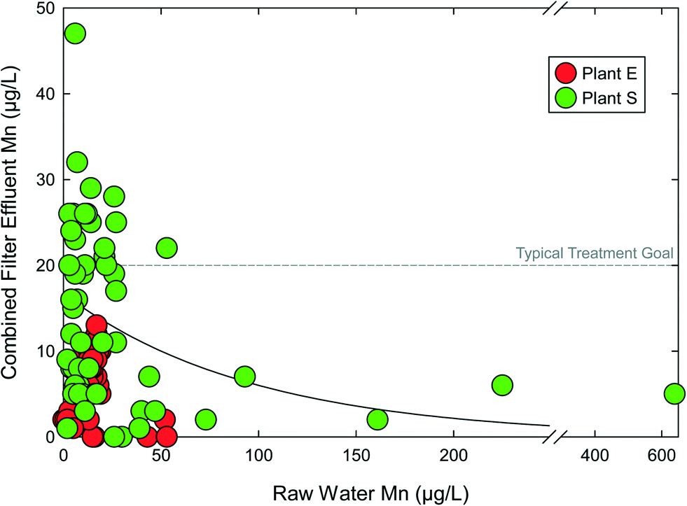 | ||
| Fig. 4 Combined filter effluent manganese (Mn) concentrations as a function of influent raw water Mn concentration for two surface water treatment plants with seasonal manganese problems. Data from Goodwill, 2006.63 | ||
The use of coagulation for the removal of DBP precursors (e.g., “enhanced coagulation” but perhaps best called “multi-objective coagulation”)67 is another example of an antifragile process common in water treatment systems. Aromatic, hydrophobic, higher molecular weight (MW) carbon compounds are more preferentially addressed by coagulation with metal salts due to charge interactions between cationic metal hydrolysis products and anionic humic macromolecules with carboxyl and phenolic groups.68,69 This is fortunate, as these same fractions of NOM also tend to have higher halogenated DBP yields due to the same unsaturated and aromatic moieties that have relatively high electron-donating capability.70,71 Therefore, as concentrations of higher DBP-forming compounds in raw water increases greater removals via enhanced coagulation are expected. This antifragile characteristic is acknowledged in the USEPA stage 1 D/DBP rule which requires higher removals of organic matter as aromatic and hydrophobic portion increases, as quantified by specific ultra-violet absorbance (SUVA).67
Incorporating the antifragility paradigm into potable water systems
Antifragility can be incorporated into a PWS by applying physicochemical processes that are known to do well under a given set of raw water quality volatility. This process requires two general steps: (1) knowledge of individual processes that increase antifragility and (2) a design evaluation approach that enable antifragile process selection under a given volatility parameter (e.g., what processes have positive convexity to this volatility parameter?). We present two examples of emerging antifragile treatment processes and describe new design tools and how they may be used. Diverging from the optimality paradigm will inherently lead to increased costs, and we also present opportunities to include real options analysis for the assessment of antifragile and financial trade-offs.Individual processes
Two examples of emerging, individual processes that may increase antifragility of PWS include: (1) ferrate (Fe(VI)) preoxidation and (2) magnetic (nano)particulate iron oxides.Fe(VI), a high-valent oxo-anion of iron,72 has been considered and evaluated as a potential preoxidant (i.e., occurring before the primary particle removal step) in drinking water treatment (DWT).73 Preoxidation is sometimes utilized as a response to BSEs, such as chemical spills,74 wildfires,75 and algal blooms76 to mitigate organic contaminants and/or improve downstream performance. Fe(VI) has a high reduction potential that is comparable to other strong oxidants in DWT such ozone (O3) and chlorine dioxide (ClO2).77 Similar performance in oxidative transformation of organic and inorganic targets between Fe(VI) and O3 has been noted, including DBP precursors,78 manganese,79 arsenic,80 and algal toxins.81 Unlike O3 and ClO2, however, Fe(VI) does not require on-site generation. A production method for stable, high-purity K2FeO4(s) salts has been developed,82 which forms the basis for recent commercial applications. Also Fe(VI) generally leads to lower yields of active bromide and bromate than O3,83 due to the simultaneous in situ formation of H2O2 during Fe(VI) decay,84 which reduces HOBr to Br−.85 Fe(VI) does not form chlorite or chlorate, unlike ClO2, and is not known to directly from any other regulated byproducts.72
This difference in generation between O3/ClO2 (on-site) and K2FeO4 (off-site) makes Fe(VI) a way for increasing antifragility of a PWS. K2FeO4 can be acquired as needed, stored onsite as a stable salt, and added as conditions dictate, similar to powdered activated carbon usage for managing urgent events. However, Fe(VI) leads to benefits to multiple water treatment physicochemical processes including (pre)oxidation, coagulation, clarification, and disinfection.73,86 These multimodal benefits enable production of water quality better than baseline, in spite of a sudden deterioration in raw water quality. For example, bench-scale testing has demonstrated lower post-clarification water turbidities following an algae spike than was otherwise achievable.87 Similar results related to ferrate use in natural disaster emergency contexts have been noted at the point-of-use (POU) scale.88,89
K2FeO4 dissolves in water to produce Fe(VI) which is a relatively strong oxidant, leading to the transformation of various reduced targets stemming from a BSE including algae and algal toxins,90,91 chemical spills (e.g., methyl tert-butyl ether).92 This Fe(VI) can also be activated using common shelf-stable reductants, such as sulfite, forming radicals Fe(V) and SO4˙−in situ that are capable of transforming recalcitrant organics.93,94 Following oxidation, Fe(VI/V) is reduced to Fe(III) which is insoluble in most water treatment contexts. These in situ formed iron particles have unique characteristics including polydisperse diameters,95 magnetism,96 and core–shell architecture.97 Ferrate resultant particles then participate in coagulation,98 flocculation,91 clarification, and adsorption processes.97,99 This multimodal action enables antifragility in response to volatility. For example, a water utility experiencing an unforeseen chemical spill could deploy ferrate as needed to oxidize the pollutant, while simultaneously decreasing disinfection byproducts, and improving coagulation beyond typical baseline operations. Thus, the as needed deployment of shelf stable K2FeO4 as represents a step towards antifragility. In contrast to MnOx, Fe(VI)-derived benefits are from the use of the technology itself, not a synergistic effect of the degraded water quality. Fe(VI), in several forms, could also be conducive to consistent use as part of baseline operations.
Iron oxide nanoparticles (IONPs), exclusive of the ferrate context, also provide antifragility to PWS through the combination of adsorption and magnetic separation.100 Iron oxide nanoparticles comprised of magnetite (Fe3O4) or maghemite (γ-Fe2O3) exhibit superparamagnetic properties and relatively high adsorption capacities for various drinking water contaminants. These IONPs can be synthesized off site, stored and used as needed by a PWS, like powdered activated carbon. However, unlike PAC, IONPs can be selectively recovered via magnetic separation, and reused.101 IONPs were found to decrease the concentration rhodamine B dye in aqueous solution by >60% with no significant decrease in adsorption capacity after five cycles of magnetic separation and chemical regeneration. Magnetic-based separations have demonstrated effectiveness of >95%, using commercially available permanent magnet systems.101,102 The use of magnets may also improve flocculation and separation of non-magnetic particles assuming attachment to an IONP. Magnetic attraction between superparamagnetic IONPs in a magnetic field would serve to increase aggregation rate from a DLVO perspective. Therefore, addition of IONPs in response to an algal bloom, forest fire, or chemical spill could enable improved water quality more than if the BSE had not occurred. For example, modeling magnetic filtration of activated sludge particles comprised of 10% IONPs by volume with stainless steel wool (M = 0.2 T) indicate filtration performance 100 times more effective than a conventional gravity filter with media collectors.103 In this way, IONPs represent a “switch on” method for achieving antifragility (similar to K2FeO4); however, they may also be used outside of periods of volatile water quality and provide benefits during more typical periods.
Design tools
A water system designer interested in incorporating antifragile processes into a drinking water plant requires new tools for guidance and evaluation. Current and historical process design under the optimality paradigm follows a multistep deterministic approach: (1) characterization of raw water quality and establishment of treatment goals; (2) jar testing and pilot studies and (3) selection of treatment processes optimized to conditions during jar testing and piloting. This approach produces treatment facilities that are generally minimized for cost given a required baseline performance. However, a six month pilot test has a low probability of evaluating a BSE, and the system design has opacity to what future conditions a particular process might need to be antifragile to. In other words, incorporation of antifragile processes requires a lens to systematically evaluate weakness prior to picking antifragile processes. This establishes a potentially beneficial relationship with future volatility that is a key characteristic of an antifragile system.29Artificial neural networks (ANNs) are a biologically-inspired computational model generally consisting of an input layer, hidden layer(s), and an output layer.104 There are many different forms of ANNs and their corresponding models are trained and built using multiple methods and calibrated using large data sets such that the weights between different neurons and hidden layers can be estimated.105 ANNs offer several advantages over traditional modeling approaches and are well-suited for drinking water treatment applications because: (1) associations between inputs and outputs are “learned” from historical data without having to specify the form of the model; (2) results of ANN runs are robust to noisy or discontinuous data; (3) a detailed understanding of the processes (i.e., treatment process) is not necessary, only an understanding of the factors that influence the processes; and (4) they are fast (increases in computer processing speeds have reduced the time needed to train and evaluate these models).106,107 For example, Zhang et al. 2004 (ref. 105) used an ANN for modelling a full-scale drinking water treatment facility lime clarification process and reported r-squared value of 0.92 for the ANN model versus 0.41 for the USEPA Water Treatment Plant Model. ANNs have been used for simultaneous prediction of turbidity and DOC removal for a conventional surface water treatment plant configuration as a function of source water quality parameters and chemical use.108 Results from Kennedy et al., 2015 (ref. 108) indicate that ANNs can be used to provide an evaluation of the impact on DOC changes (as measured by individual parallel factor analysis components) on the coagulation process and turbidity removal. This enables virtual jar testing of future water quality scenarios that were not present during the original experiments. Coagulation of the turbidity and/or DOC event caused by a BSE (e.g., wildfire, accelerating lake recovery, or hurricane) can be evaluated prior to occurrence, allowing for development of antifragile elements into the physicochemical processes. In other words, shifts in water quality presented in Fig. 1 could be simulated to “stress test” and assess impact on coagulation/clarification performance before they occur, and identify potential chemical combinations and operational settings that perform better as the same shifts occur.
Beyond bench-scale, pilot testing can also be improved with digital tools to achieve antifragility, primarily by simulating performance during extreme events prior to their occurrence. Developments in pilot-testing have led to the development of “proven perfect” pilot-scale systems that closely replicate their full-scale counterparts, as demonstrated by paired t tests to confirm the production of statistically equivalent water quality.109 Knowles et al., 2012 (ref. 109) describes this process for the JDKWSP. This particular pilot system has been used to established possible physicochemical solutions to lake recovery, albeit after the negative impacts from lake recovery were realized.44 Pilot-scale systems that are proven to represent full-scale performance can be combined with digital twins to “stress test” a proposed process system design before problems arise, and proactively select and incorporate antifragile processes. A digital twin is a dynamic simulation model that visually integrates system components, and can be combined with data variations to understand the sensitivity of a physical system to input perturbation.110
Essentially, these digital twins enable the typical process design question to be flipped: what types of future BSEs is the system fragile (e.g., negative convexity)? Curl et al. 2020 (ref. 110) refers to this approach as “failure analysis”. In this application the failure is virtual, and information generated can be used to select processes that would perform better when the same BSE occurs (e.g., positive convexity). In this way the designer is empowered to systematically increase the antifragility of a water treatment system. The drinking water treatment space is currently experiencing early adoption of digital twins. For example, the City of San Diego (California, USA) is developing a digital twin of its North City Pure Water Facility, a component of their water reuse program.110 This digital twin operates via one second time steps, and fully replicates system hydraulics and process performance. The city intends to employ the digital twin to improve future performance to operational challenges.
Investment considerations
Investments in antifragility may require capital cost outlays, behavioral changes and localized downtime or inconvenience as systems are altered from the original deterministic designs. Investment in antifragility therefore requires demonstration of benefits that outweigh the costs – benefits such as improved performance, increased long-term (i.e., intergenerational) water security. Tradeoff analysis such as this is the realm of decision science, and the application to antifragility investment follows.Tradeoff analysis is the analytical core of Decision Making under Deep Uncertainty.111Fig. 5 summarizes one approach. For the sake of illustration, we select four desired attributes of the proposed water treatment system: (1) low capital cost; (2) low operating costs; (3) high baseline performance; and (4) low fragility. The three design options in this case, as presented in Fig. 1, are direct filtration (DF), sedimentation (Sed.), and dissolved air flotation (DAF). In the illustration, DF has the lowest capital costs and sedimentation has the highest capital costs. Why, then, would one choose to build sedimentation over DF? One motivating factor might be the higher baseline performance offered by sedimentation. But that baseline performance is calculated, as previously discussed in the Design considerations section above, with reference to the particular raw water characteristics observed in the historical case, and it changes depending on whether the designer believes that those historical raw water characteristics will continue into the future or shift in some anticipatable fashion. Shifts in raw water characteristics will affect estimates of operating costs, and the system fragility.
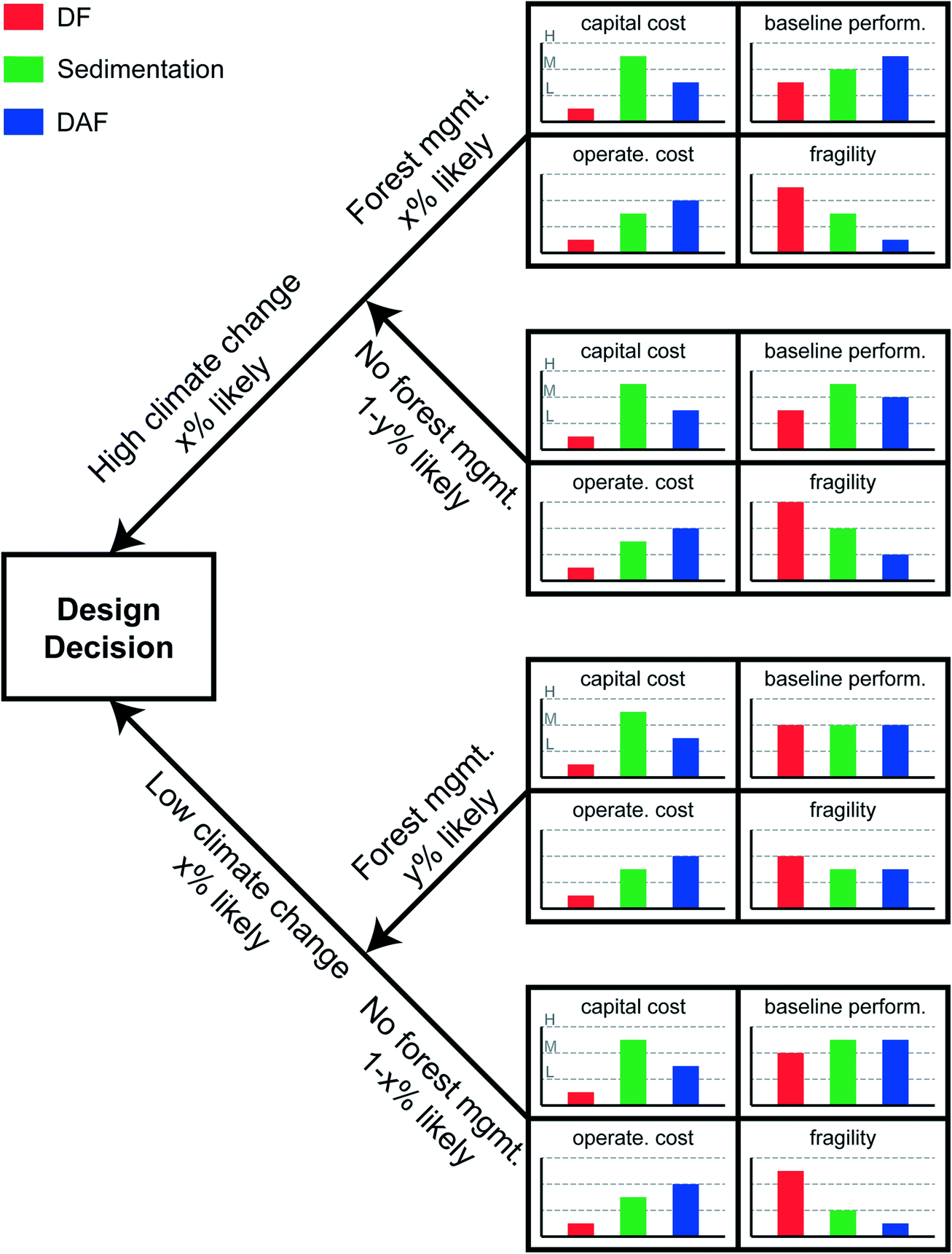 | ||
| Fig. 5 Real options analysis decision tree framework for the comparison of three clarification designs: direct filtration (DF), gravity sedimentation (e.g., conventional settling), and dissolved air flotation (DAF). Capital and operational costs, and baseline performance taken from Gregory and Edzwald, 2011.42 | ||
One method for navigating uncertainty in future raw water characteristics when designing a water system is to enumerate a decision tree.112 This approach, sometimes referred to (especially in applications to financial decision making) as real options analysis (ROA, see for example Ranger et al. (2010)),113 involves stepping through branches of distinct uncertainties. Each uncertainty is discretized into easily understood categories of exogenous variable such as “high”, “medium”, or “low”. Endogenous variables (such as “build this” or “build X amount of that” or “don't build”) are decision points at the left-hand side of decision trees. In higher-order complex decision trees, endogenous decision points can be interspersed throughout the branches of the tree to represent decision staging and adaptive design. Fig. 5 includes only a single endogenous decision point (build DF or sedimentation or DAF), and two exogenous variables to which the performance of the treatment plant is sensitive: climate change, discretized into “high”, signifying rapid global warming over the treatment plant's design life, and “low” signifying less rapid global warming; and forest management, discretized into “yes” or “no”. Climate change increases ambient air temperatures and speeds the hydrologic cycle, resulting in lower base flows during dry periods and higher velocity flow during wet periods. Each condition creates raw water quality challenges, as described in the Introduction. Forest management is costly (and controversial), but has potential to reduce evapotranspiration, reduce forest fire risks, and improve soil retention. Forest management also benefits source water protection,114 which can be considered the first step in water treatment,115 from a multiple barrier perspective by decreasing contaminant load in source waters. For the sake of illustration, these two variables are presented as independent, i.e., forest management policy has no bearing on climate change magnitude, and climate change magnitude has no bearing on forest management policy.
Scenarios are formulated as combinations of the fully enumerated decision tree, in this case: high climate change and forest management, high climate change without forest management, low climate change and forest management, low climate change without forest management. Once the scenarios are enumerated, variable values (e.g., water temperature, sediment load) are assigned to represent each condition, and the performance of each treatment option is simulated for each variable setting. Simulations might be accomplished with an ANN, a physically based model, or a “digital twin”, as discussed earlier. As shown in Fig. 5, the baseline performance of each treatment option is differently responsive to the altered conditions. In the case of low climate change and forest management, DF might be the preferred choice as it is lowest in cost with comparable baseline performance, and only slightly elevated fragility. However, in the case of high climate change and no forest management, sedimentation might be the preferred choice, with its high baseline performance and relatively low fragility. DAF appears the best option in the case of low climate change without forest management, with its moderate costs, high baseline performance and very low fragility. Probabilistic weighting and risk hedging is needed before a final decision can be made.
Climate change carries deep uncertainty. The Intergovernmental Panel on Climate Change (IPCC) Sixth Assessment Report presents possible climate futures as a function of potential reductions in carbon dioxide and other greenhouse gas emissions. The extent of realized global warming will affect the climate system in numerous ways, including precipitation extremes, and more intense tropic cyclones.116 It is impossible to know whether “high” climate change or “low” will occur, and it is impossible to know whether the next set of politicians will opt for forest management or not. However, in order to overcome the paralysis created by the uncertainty regarding future watershed conditions, we weight possible future conditions by likelihood of occurrence and calculate the expected value of each performance metric across the uncertainty space as shown in eqn (1).
| ξ = ∑s∈Ωpsξs ∀s | (1) |
Expected values are not the only metrics of interest and depending on the risk aversion (or relative optimism) of the particular decision maker, there might be more or less focus placed on extreme values – best-case and worst-case performance of each water treatment plant design option. Finally, likelihoods could be assigned in this case, for example, by consulting the most up-to-date science on global climate change produced by the IPCC, and local experts on the history and likely future management of local forests. The process of likelihood weighting is inexact, and best subjected to sensitivity analysis (i.e., repeated evaluation changing likelihoods and re-determining the preferred decision). See Ray et al. (2012) for an example exploration of the sensitivity of staged climate change adaptation decisions to changes in scenario likelihoods.117
Conclusion
The deterministic approach to drinking water system design has served society well and led to safe supplies of water at low costs; however, these optimized water systems carry the indirect cost of fragility. This fragility has become increasingly problematic as source water volatility and other extreme events have increased. This increased variability makes reliance on stationarity unsustainable. Water system design has begun to increase emphasis on resilience, although this paradigm still has an adversarial relationship with volatility. Pursuing antifragility in water systems creates a different relationship with change, whereby system processes are placed in a position to perform better as conditions change with less reliance on future forecasts. Processes conveying antifragility can be included into PWS designs by new tools powered by ANNs, including virtual jar and pilot testing, that allow for systematic evaluation of convexity. Including antifragile components into a PWS will inherently cost more than an option optimized for lowest cost. Therefore, developing antifragile characteristics represents a trade-off between performance and cost. Real options analysis is one way for water system designers to consider this trade-off. Ultimately, more research on antifragile designs and costs is required to ensure long-term performance and sustainability of public water systems in an era of increasing volatility.Conflicts of interest
There are no conflicts of interest to declare.References
- D. Schoenen, Role of Disinfection in Suppressing the Spread of Pathogens with Drinking Water: Possibilities and Limitations, Water Res., 2002, 36(15), 3874–3888, DOI:10.1016/S0043-1354(02)00076-3.
- B. Lykins and R. Clark, US Drinking Water Regulations: Treatment Technologies and Cost, Environ. Eng., 1994, 120(4), 783–802 CrossRef CAS.
- A. J. Whelton, L. K. McMillan, M. Connell, K. M. Kelley, J. P. Gill, K. D. White, R. Gupta, R. Dey and C. Novy, Residential Tap Water Contamination Following the Freedom Industries Chemical Spill: Perceptions, Water Quality, and Health Impacts, Environ. Sci. Technol., 2015, 49(2), 813–823, DOI:10.1021/es5040969.
- B. W. Brooks, J. M. Lazorchak, M. D. A. Howard, M.-V. V. Johnson, S. L. Morton, D. A. K. Perkins, E. D. Reavie, G. I. Scott, S. A. Smith and J. A. Steevens, Are Harmful Algal Blooms Becoming the Greatest Inland Water Quality Threat to Public Health and Aquatic Ecosystems?, Environ. Toxicol. Chem., 2016, 35(1), 6–13, DOI:10.1002/etc.3220.
- H. Majidzadeh, H. Uzun, H. Chen, S. Bao, M. T. K. Tsui, T. Karanfil and A. T. Chow, Hurricane Resulted in Releasing More Nitrogenous than Carbonaceous Disinfection Byproduct Precursors in Coastal Watersheds, Sci. Total Environ., 2019, 705, 1–9, DOI:10.1016/j.scitotenv.2019.135785.
- M. W. LeChevallier, The Impact of Climate Change on Water Infrastructure, J. - Am. Water Works Assoc., 2014, 106(4), 79–81 CrossRef CAS.
- A. K. Hohner, R. S. Summers and F. L. Rosario-Ortiz, Laboratory Simulation of Postfire Effects on Conventional Drinking Water Treatment and Disinfection Byproduct Formation, AWWA Water Sci., 2019, 1(5), 1–17, DOI:10.1002/aws2.1155.
- A. K. Hohner, K. Cawley, J. Oropeza, R. S. Summers and F. L. Rosario-Ortiz, Drinking Water Treatment Response Following a Colorado Wildfire, Water Res., 2016, 105, 187–198, DOI:10.1016/j.watres.2016.08.034.
- D. González-Zeas, B. Erazo, P. Lloret, B. De Bièvre, S. Steinschneider and O. Dangles, Linking Global Climate Change to Local Water Availability: Limitations and Prospects for a Tropical Mountain Watershed, Sci. Total Environ., 2019, 650, 2577–2586, DOI:10.1016/j.scitotenv.2018.09.309.
- K. M. Faust, D. M. Abraham and S. P. McElmurry, Water and Wastewater Infrastructure Management in Shrinking Cities, Public Works Manag. Policy, 2016, 21(2), 128–156, DOI:10.1177/1087724X15606737.
- V. Morckel, Why the Flint, Michigan, USA Water Crisis Is an Urban Planning Failure, Cities, 2017, 62, 23–27, DOI:10.1016/j.cities.2016.12.002.
- P. A. Ray and C. M. Brown, Confronting Climate Uncertainty in Water Resources Planning and Project Design: The Decision Tree Framework, The World Bank, 2015, DOI:10.1596/978-1-4648-0477-9.
- D. Elder and G. Budd, Overview of Water Treatment Processes, in Water Quality & Treatment: A Handbook on Drinking Water, ed. J. K. Edzwald, AWWA, McGraw Hill, Denver, CO, 2011, p. 38 Search PubMed.
- M. R. Wiesner, C. R. O'Melia and J. L. Cohon, Optimal Water Treatment Plant Design, J. Environ. Eng., 1987, 113(3), 567–584, DOI:10.1061/(ASCE)0733-9372(1987)113:3(567).
- J. O. Tijani, O. O. Fatoba, O. O. Babajide and L. F. Petrik, Pharmaceuticals, Endocrine Disruptors, Personal Care Products, Nanomaterials and Perfluorinated Pollutants: A Review, Environ. Chem. Lett., 2016, 14(1), 27–49, DOI:10.1007/s10311-015-0537-z.
- D. L. Boccelli, M. J. Small and U. M. Diwekar, Drinking Water Treatment Plant Design Incorporating Variability and Uncertainty, J. Environ. Eng., 2007, 133(3), 303–312, DOI:10.1061/(ASCE)0733-9372(2007)133:3(303).
- S. Chowdhury, Decision Making with Uncertainty: An Example of Water Treatment Approach Selection, Water Qual. Res. J. Can., 2012, 47(2), 153–165, DOI:10.2166/wqrjc.2012.107.
- B. Lamrini, E. K. Lakhal and M. V. Le Lann, A Decision Support Tool for Technical Processes Optimization in Drinking Water Treatment, Desalin. Water Treat., 2014, 52(22–24), 4079–4088, DOI:10.1080/19443994.2013.803327.
- A. M. Michalak, Study Role of Climate Change in Extreme Threats to Water Quality, Nature, 2016, 535, 349 CrossRef CAS PubMed.
- P. C. D. Milly, J. Betancourt, M. Falkenmark, R. M. Hirsch, Z. W. Kundzewicz, D. P. Lettenmaier, R. J. Stouffer, M. D. Dettinger and V. Krysanova, Stationarity Is Dead: Whither Water Management?, Water Resour. Res., 2015, 319(51), 9207–9231, DOI:10.1002/2015WR017408 . Received.
- H. A. Lempert, R. Brown, C. Gill and S. S. Stuart, Investment Decision Making under Deep Uncertainty - Application to Climate Change, The World Bank, 2012, DOI:10.1596/1813-9450-6193.
- W. J. Raseman, J. R. Kasprzyk, F. L. Rosario-Ortiz, J. R. Stewart and B. Livneh, Emerging Investigators Series: A Critical Review of Decision Support Systems for Water Treatment: Making the Case for Incorporating Climate Change and Climate Extremes, Environ. Sci.: Water Res. Technol., 2017, 3(1), 18–36, 10.1039/c6ew00121a.
- P. P. Rogers and M. B. Fiering, Use of Systems Analysis in Water Management, Water Resour. Res., 1986, 22(9 S), 146S–158S, DOI:10.1029/WR022i09Sp0146S.
- A. D. Levine, Y. J. Yang and J. A. Goodrich, Enhancing Climate Adaptation Capacity for Drinking Water Treatment Facilities, Environ. Sci.: Water Res. Technol., 2016, 7(3), 485–497, DOI:10.2166/wcc.2016.011.
- C. Brown, F. Boltz, S. Freeman, J. Tront and D. Rodriguez, Resilience by Design: A Deep Uncertainty Approach for Water Systems in a Changing World, Water Secur., 2020, 9, 100051, DOI:10.1016/j.wasec.2019.100051.
- NIAC, Crticial Infrastructure Resilience Final Report and Recommendations, 2009 Search PubMed.
- J. Baylis, A. Edmons, M. Grayson, J. Murren, J. McDonald and B. Scott, NIAC Water Sector Resilience: Final Report and Recommendations, Washington, DC, 2016 Search PubMed.
- K. M. Morley, Priority Action on Risk and Resilience, J. - Am. Water Works Assoc., 2019, 111(2), 12–12, DOI:10.1002/awwa.1229.
- N. N. Taleb, Antifragile: Things That Gain from Disorder, Random House Incorporated, 2012, vol. 3 Search PubMed.
- K. H. Jones, Engineering Antifragile Systems: A Change in Design Philosophy, Procedia Comput. Sci., 2014, 32(Antifragile), 870–875, DOI:10.1016/j.procs.2014.05.504.
- N. N. Taleb, The Black Swan: The Impact of the Highly Improbable, Random house, 2nd edn, 2007 Search PubMed.
- B. Mandelbrot, The Variation of Certain Speculative Prices, J. Bus., 1963, 36, 394–419, DOI:10.1142/9789814566926_0003.
- N. N. Taleb, Black Swans and the Domains of Statistics, Am. Stat., 2007, 61(3), 198–200, DOI:10.1198/000313007X219996.
- L. E. Anderson, W. H. Krkošek, A. K. Stoddart, B. F. Trueman and G. A. Gagnon, Lake Recovery Through Reduced Sulfate Deposition: A New Paradigm for Drinking Water Treatment, Environ. Sci. Technol., 2017, 51(3), 1414–1422, DOI:10.1021/acs.est.6b04889.
- W. C. Becker, A. Hohner, F. Rosario-Ortiz and J. DeWolfe, Preparing for Wildfires and Extreme Weather: Plant Design and Operation Recommendations, J. - Am. Water Works Assoc., 2018, 110(7), 32–40, DOI:10.1002/awwa.1113.
- H. Chen, H. Uzun, A. T. Chow and T. Karanfil, Low Water Treatability Efficiency of Wildfire-Induced Dissolved Organic Matter and Disinfection by-Product Precursors, Water Res., 2020, 116111, DOI:10.1016/j.watres.2020.116111.
- H. Paerl and J. Huisman, Blooms Like It Hot, Science, 2008, 320, 57–58, DOI:10.1126/science.1155398.
- M. E. Thompson and M. B. Hutton, Sulfate in Lakes of Eastern Canada: Calculated Yields Compared with Measured Wet and Dry Deposition, Water, Air, Soil Pollut., 1985, 24(1), 77–83, DOI:10.1007/BF00229520.
- J. H. Writer, A. Hohner, J. Oropeza, A. Schmidt, K. Cawley and F. L. Rosario-Ortiz, Water Treatment Implications after the High Park Wildfire in Colorado, J. - Am. Water Works Assoc., 2014, 106(4), 85–86, DOI:10.5942/jawwa.2014.106.0055.
- A. K. Hohner, K. Cawley, J. Oropeza, R. S. Summers and F. L. Rosario-Ortiz, Drinking Water Treatment Response Following a Colorado Wildfire, Water Res., 2016, 105, 187–198, DOI:10.1016/j.watres.2016.08.034.
- M. T. Valade, W. C. Becker and J. K. Edzwald, Treatment Selection Guidelines for Particle and NOM Removal, J. - Am. Water Works Assoc., 2009, 58(6), 424–432, DOI:10.2166/aqua.2009.201.
- R. Gregory and J. K. Edzwald, Sedimentaation and Flotation, in Water Quality & Treatment: A Handbook on Drinking Water, ed. J. K. Edzwald, AWWA, McGraw Hill, Denver, CO, 2011, pp. 9.1–9.89 Search PubMed.
- J. K. Edzwald, Dissolved Air Flotation and Me, Water Res., 2010, 44(7), 2077–2106, DOI:10.1016/j.watres.2009.12.040.
- I. DeMont, A. K. Stoddart and G. A. Gagnon, Assessing Strategies to Improve the Efficacy and Efficiency of Direct Filtration Plants Facing Changes in Source Water Quality from Anthropogenic and Climatic Pressures, J. Water Process. Eng., 2020, 101689, DOI:10.1016/j.jwpe.2020.101689.
- A. D. Knowles, C. K. Nguyen, M. A. Edwards, A. Stoddart, B. McIlwain and G. A. Gagnon, Role of Iron and Aluminum Coagulant Metal Residuals and Lead Release from Drinking Water Pipe Materials, J. Environ. Sci. Health, Part A: Toxic/Hazard. Subst. Environ. Eng., 2015, 50(4), 414–423, DOI:10.1080/10934529.2015.987550.
- P. Langley, Anticipating Uncertainty, Reviving Risk? On the Stress Testing of Finance in Crisis, Econ. Soc., 2013, 42(1), 51–73, DOI:10.1080/03085147.2012.686719.
- N. N. Taleb and R. Douady, Mathematical Definition, Mapping, and Detection of (Anti)Fragility, Quant. Finance, 2013, 13(11), 1677–1689, DOI:10.1080/14697688.2013.800219.
- N. N. Taleb, E. Canetti, T. Kinda, E. Loukoianova and C. Schmieder, A New Heuristic Measure of Fragility and Tail Risks: Application to Stress Testing, IMF Working Paper 12/216, 2012, vol. 2012 Search PubMed.
- J. K. Edzwald, Algae, Bubbles, Coagulants and Dissolved Air Flotation, Water Sci. Technol., 1993, 27(10), 67–81 CrossRef CAS.
- Providence Water, Annual Water Quality Report, Providence, 2018 Search PubMed.
- D. A. Reckhow and P. C. Singer, Chlorination By-Products in Drinking Waters. From Formation Potentials to Finished Water Concentrations, J. - Am. Water Works Assoc., 1990, 82(4), 173–180, DOI:10.1108/EJTD-03-2013-0030.
- B. Chen and P. Westerhoff, Predicting Disinfection By-Product Formation Potential in Water, Water Res., 2010, 44(13), 3755–3762, DOI:10.1016/j.watres.2010.04.009.
- J. K. Edzwald, W. C. Becker and K. L. Wattier, Surrogate Parameters for Monitoring Organic Matter and THM Precursors, J. - Am. Water Works Assoc., 1985, 77(4), 122–131 CrossRef CAS.
- F. Babovic, V. Babovic and A. Mijic, Antifragility and the Development of Urban Water Infrastructure, Int. J. Water Resour. Dev., 2017, 0627, 1–11, DOI:10.1080/07900627.2017.1369866.
- T. H. F. Wong and R. R. Brown, The Water Sensitive City: Principles for Practice, Water Sci. Technol., 2009, 60(3), 673–682, DOI:10.2166/wst.2009.436.
- R. R. Brown, N. Keath and T. H. F. Wong, Urban Water Management in Cities: Historical, Current and Future Regimes, Water Sci. Technol., 2009, 59(5), 847–855, DOI:10.2166/wst.2009.029.
- S. Bird and C. Hotaling, Multi-Stakeholder Microgrids for Resilience and Sustainability, Environ. Hazards, 2017, 16(2), 116–132, DOI:10.1080/17477891.2016.1263181.
- D. Nock and E. Baker, Unintended Consequences of Northern Ireland's Renewable Obligation Policy, Electr. J., 2017, 30(7), 47–54, DOI:10.1016/j.tej.2017.07.002.
- M. Panteli, D. N. Trakas, P. Mancarella and N. D. Hatziargyriou, Boosting the Power Grid Resilience to Extreme Weather Events Using Defensive Islanding, IEEE Trans. Smart Grid, 2016, 7(6), 2913–2922, DOI:10.1109/TSG.2016.2535228.
- J. E. Tobiason, A. Bazilio, J. Goodwill, X. Mai and C. Nguyen, Manganese Removal from Drinking Water Sources, Curr. Pollut. Rep., 2016, 1–10, DOI:10.1007/s40726-016-0036-2.
- A. M. Dietrich and G. A. Burlingame, Critical Review and Rethinking of USEPA Secondary Standards for Maintaining Organoleptic Quality of Drinking Water, Environ. Sci. Technol., 2015, 49(2), 708–720, DOI:10.1021/es504403t.
- P. Brandhuber, S. Clark, W. Knocke and J. Tobiason, Guidance for the Treatment of Manganese, Water Research Foundation, Denver, CO, 2013 Search PubMed.
- J. Goodwill, Characterization of Manganese Oxide Coated Filter Media, 2006 Search PubMed.
- W. R. Knocke, R. C. Hoehn and R. L. Sinsabaugh, Using Alternative Oxidants to Remove Dissolved Manganese from Waters Laden with Organics, J. - Am. Water Works Assoc., 1987, 79(3), 75–79 CrossRef CAS.
- A. A. Islam, J. E. Goodwill, R. Bouchard, J. E. Tobiason and W. R. Knocke, Characterization of Filter Media MnOX(S) Surfaces and Mnremoval Capability, J. - Am. Water Works Assoc., 2010, 102(9), 71–83 CrossRef CAS.
- J. E. Tobiason, W. R. Knocke, J. Goodwill, P. Hargette, R. Bouchard and L. Zuravnsky, Characterization and Performance of Filter Media for Manganese Control, Water Research Foundation, Denver, CO, 2008 Search PubMed.
- J. K. Edzwald and J. E. Tobiason, Enhanced Coagulation: US Requirements and a Broader View, Water Sci. Technol., 1999, 40(9), 63–70, DOI:10.1016/S0273-1223(99)00641-1.
- J. E. Van Benschoten and J. K. Edzwald, Chemical Aspects of Coagulation Using Aluminum Salts - I. Hydrolytic Reactions of Alum and Polyaluminum Chloride, Water Res., 1990, 24(12), 1519–1526, DOI:10.1016/0043-1354(90)90086-L.
- M. Edwards, Predicting DOC Removal during Enhanced Coagulation, J. - Am. Water Works Assoc., 1997, 89(5), 78–89, DOI:10.1002/j.1551-8833.1997.tb08229.x.
- M. C. Kavanaugh, Modified Coagulation for Improved Removal of Trihalomethane Precursors, J. - Am. Water Works Assoc., 1978, 70(11), 613–620 CrossRef CAS.
- D. A. Reckhow and P. C. Singer, The Removal of Organic Halide Precursors by Preozonation and Alum Coagulation, J. - Am. Water Works Assoc., 1984, 76(4), 151–157, DOI:10.2307/41272010.
- V. K. Sharma, L. Chen and R. Zboril, Review on High Valent FeVI (Ferrate): A Sustainable Green Oxidant in Organic Chemistry and Transformation of Pharmaceuticals, ACS Sustainable Chem. Eng., 2016, 4(1), 18–34, DOI:10.1021/acssuschemeng.5b01202.
- J. E. Goodwill, Y. Jiang, D. A. Reckhow and J. E. Tobiason, Laboratory Assessment of Ferrate for Drinking Water Treatment, J. - Am. Water Works Assoc., 2016, 108(3), 164–174, DOI:10.5942/jawwa.2016.108.0029.
- P. K. A. Hong and T. Xiao, Treatment of Oil Spill Water by Ozonation and Sand Filtration, Chemosphere, 2013, 91(5), 641–647, DOI:10.1016/j.chemosphere.2013.01.010.
- A. K. Hohner, L. G. Terry, E. B. Townsend, R. S. Summers and F. L. Rosario-Ortiz, Water Treatment Process Evaluation of Wildfire-Affected Sediment Leachates, Environ. Sci.: Water Res. Technol., 2017, 3(2), 352–365, 10.1039/c6ew00247a.
- J. D. Plummer and J. K. Edzwald, Effect of Ozone on Algae as Precursors for Trihalomethane and Haloacetic Acid Production, Environ. Sci. Technol., 2001, 35(18), 3661–3668, DOI:10.1021/es0106570.
- V. K. Sharma, F. Kazama, H. Jiangyong and A. K. Ray, Ferrates (Iron(VI) and Iron(V)): Environmentally Friendly Oxidants and Disinfectants, J. Water Health, 2005, 3(1), 45–58 CrossRef CAS.
- Y. Jiang, J. E. Goodwill, D. A. Reckhow and J. E. Tobiason, Impacts of Ferrate Oxidation on Natural Organic Matter and Disinfection Byproduct Precursors, Water Res., 2016, 96, 114–125, DOI:10.1016/j.watres.2016.03.052.
- J. E. Goodwill, X. Mai, Y. Jiang, D. A. Reckhow and J. E. Tobiason, Oxidation of Manganese (II) with Ferrate: Stoichiometry, Kinetics, Products, and Impact of Organic Carbon, Chemosphere, 2016, 159, 457–464, DOI:10.1016/j.chemosphere.2016.06.014.
- Y. Lee, I. Um and J. Yoon, Arsenic(III) Oxidation by Iron(VI) (Ferrate) and Subsequent Removal of Arsenic(V) by Iron(III) Coagulation, Environ. Sci. Technol., 2003, 37(24), 5750–5756 CrossRef CAS PubMed.
- A. Islam, D. Jeon, J. Ra, J. Shin, T. Y. Kim and Y. Lee, Transformation of Microcystin-LR and Olefinic Compounds by Ferrate(VI): Oxidative Cleavage of Olefinic Double Bonds as the Primary Reaction Pathway, Water Res., 2018, 141, 268–278, DOI:10.1016/j.watres.2018.05.009.
- B. F. Monzyk, J. K. Rose, E. C. Burckle, A. D. Smeltz, D. G. Rider, C. M. Cucksey and T. O. Clark, Method for Producing Ferrate (V) and/or (VI), US8449756B2, 2013.
- Y. Jiang, J. E. Goodwill, J. E. Tobiason and D. A. Reckhow, Comparison of Ferrate and Ozone Pre-Oxidation on Disinfection Byproduct Formation from Chlorination and Chloramination, Water Res., 2019, 156, 110–124, DOI:10.1016/j.watres.2019.02.051.
- Y. Lee, R. Kissner and U. von Gunten, Reaction of Ferrate(VI) with ABTS and Self-Decay of Ferrate(VI): Kinetics and Mechanisms, Environ. Sci. Technol., 2014, 48(9), 5154–5162, DOI:10.1021/es500804g.
- Y. Jiang, J. E. Goodwill, J. E. Tobiason and D. A. Reckhow, Bromide Oxidation by Ferrate(VI): The Formation of Active Bromine and Bromate, Water Res., 2016, 96, 188–197, DOI:10.1016/j.watres.2016.03.065.
- S. Daer, J. E. Goodwill and K. Ikuma, Effect of Ferrate and Monochloramine Disinfection on the Physiological and Transcriptomic Response of Escherichia Coli at Late Stationary Phase, Water Res., 2021, 189, 116580, DOI:10.1016/j.watres.2020.116580.
- Y. Deng, M. Wu, H. Zhang, L. Zheng, Y. Acosta and T. T. D. Hsu, Addressing Harmful Algal Blooms (HABs) Impacts with Ferrate(VI): Simultaneous Removal of Algal Cells and Toxins for Drinking Water Treatment, Chemosphere, 2017, 186, 757–761, DOI:10.1016/j.chemosphere.2017.08.052.
- J. Cui, L. Zheng and Y. Deng, Emergency Water Treatment with Ferrate(VI) in Response to Natural Disasters, Environ. Sci.: Water Res. Technol., 2018, 4, 359–368, 10.1039/C7EW00467B.
- L. Zheng, J. Cui and Y. Deng, Emergency Water Treatment with Combined Ferrate(vi) and Ferric Salts for Disasters and Disease Outbreaks, Environ. Sci.: Water Res. Technol., 2020, 6(10), 2816–2831, 10.1039/d0ew00483a.
- W. Jiang, L. Chen, S. R. Batchu, P. R. Gardinali, L. Jasa, B. Marsalek, R. Zboril, D. D. Dionysiou, K. E. O'Shea and V. K. Sharma, Oxidation of Microcystin-LR by Ferrate(VI): Kinetics, Degradation Pathways, and Toxicity Assessments, Environ. Sci. Technol., 2014, 48(20), 12164–12172, DOI:10.1021/es5030355.
- E. Addison, K. Gerlach, G. Santilli, C. Spellman, A. Fairbrother, Z. Shepard, J. Dudle and J. Goodwill, Physicochemical Implications of Cyanobacteria Oxidation with Fe(VI), Chemosphere, 2020, 128956, DOI:10.1016/j.chemosphere.2020.128956.
- R. C. Pepino Minetti, H. R. Macaño, J. Britch and M. C. Allende, In Situ Chemical Oxidation of BTEX and MTBE by Ferrate: PH Dependence and Stability, J. Hazard. Mater., 2017, 324, 448–456, DOI:10.1016/j.jhazmat.2016.11.010.
- J. Zhang, L. Zhu, Z. Shi and Y. Gao, Rapid Removal of Organic Pollutants by Activation Sulfite with Ferrate, Chemosphere, 2017, 186, 576–579, DOI:10.1016/j.chemosphere.2017.07.102.
- M. Feng, C. Jinadatha, T. J. McDonald and V. K. Sharma, Accelerated Oxidation of Organic Contaminants by Ferrate(VI): The Overlooked Role of Reducing Additives, Environ. Sci. Technol., 2018, 52(19), 11319–11327, DOI:10.1021/acs.est.8b03770.
- J. E. Goodwill, Y. Jiang, D. A. Reckhow, J. Gikonyo and J. E. Tobiason, Characterization of Particles from Ferrate Preoxidation, Environ. Sci. Technol., 2015, 49, 4955–4962, DOI:10.1021/acs.est.5b00225.
- B. M. Bzdyra, C. D. Spellman Jr, I. Andreu and J. E. Goodwill, Sulfite Activation Changes Character of Ferrate Resultant Particles, Chem. Eng. J., 2020, 393, 124771, DOI:10.1016/j.cej.2020.124771.
- R. P. Kralchevska, R. Prucek, J. Kolařík, J. Tuček, L. Machala, J. Filip, V. K. Sharma and R. Zbořil, Remarkable Efficiency of Phosphate Removal: Ferrate(VI)-Induced in Situ Sorption on Core-Shell Nanoparticles, Water Res., 2016, 103, 83–91, DOI:10.1016/j.watres.2016.07.021.
- D. Lv, L. Zheng, H. Zhang and Y. Deng, Coagulation of Colloidal Particles with Ferrate(Vi), Environ. Sci.: Water Res. Technol., 2018, 4(5), 701–710, 10.1039/c8ew00048d.
- R. Prucek, J. Tuček, J. Kolařík, J. Filip, Z. Marušák, V. K. Sharma and R. Zbořil, Ferrate(VI)-Induced Arsenite and Arsenate Removal by in Situ Structural Incorporation into Magnetic Iron(III) Oxide Nanoparticles, Environ. Sci. Technol., 2013, 47(7), 3283–3292, DOI:10.1021/es3042719.
- X. Qu, J. Brame, Q. Li and P. J. J. Alvarez, Nanotechnology for a Safe and Sustainable Water Supply: Enabling Integrated Water Treatment and Reuse, Acc. Chem. Res., 2013, 46(3), 834–843, DOI:10.1021/ar300029v.
- C. D. Powell, A. J. Atkinson and Y. Ma, et al., Magnetic Nanoparticle Recovery Device (MagNERD) Enables Application of Iron Oxide Nanoparticles for Water Treatment, J. Nanopart. Res., 2020, 22(2), 48, DOI:10.1007/s11051-020-4770-4.
- C. T. Yavuz, J. T. Mayo, W. W. Yu, A. Prakash, J. C. Falkner, S. Yean, L. Cong, H. J. Shipley, A. Kan, M. Tomson, D. Natelson and V. L. Colvin, Low-Field Magnetic Separation of Monodisperse Fe3O4 Nancrystals, Science, 2006, 314(5801), 964–967, DOI:10.1126/science.1131475.
- J. H. P. Watson, Magnetic Filtration, J. Appl. Phys., 1973, 44(9), 4209–4213, DOI:10.1063/1.1662920.
- G. M. Foody and M. K. Arora, An Evaluation of Some Factors Affecting the Accuracy of Classification by an Artificial Neural Network, Int. J. Remote Sens., 1997, 18(4), 799–810, DOI:10.1080/014311697218764.
- Q. J. Zhang, A. A. Cudrak, R. Shariff and S. J. Stanley, Implementing Artificial Neural Network Models for Real-Time Water Colour Forecasting in a Water Treatment Plant, J. Environ. Eng. Sci., 2004, 3(Supplement 1), S15–S23, DOI:10.1139/s03-066.
- C. W. Baxter, Q. Zhang, S. J. Stanley, R. Shariff, R.-R. T. Tupas and H. L. Stark, Drinking Water Quality and Treatment: The Use of Artificial Neural Networks, Can. J. Civ. Eng., 2001, 28(S1), 26–35, DOI:10.1139/cjce-28-s1-26.
- Q. Zhang and S. J. Stanley, Real-Time Water Treatment Process Control with Artifical Neural Networks, J. Environ. Eng., 1999, 125(2), 153–160 CrossRef CAS.
- M. J. Kennedy, A. H. Gandomi and C. M. Miller, Coagulation Modeling Using Artificial Neural Networks to Predict Both Turbidity and DOM-PARAFAC Component Removal, J. Environ. Chem. Eng., 2015, 3(4), 2829–2838, DOI:10.1016/j.jece.2015.10.010.
- A. D. Knowles, J. Mackay and G. A. Gagnon, Pairing a Pilot Plant to a Direct Filtration Water Treatment Plant, Can. J. Civ. Eng., 2012, 39(6), 689–700, DOI:10.1139/L2012-060.
- J. M. Curl, T. Nading, K. Hegger, A. Barhoumi and M. Smoczynski, Digital Twins: The Next Generation of Water Treatment Technology, J. - Am. Water Works Assoc., 2019, 111(12), 44–50, DOI:10.1002/awwa.1413.
- Decision Making under Deep Uncertainty: From Theory to Practice, ed. V. A. W. J. Marchau, W. E. Walker, P. J. T. M. Bloemen and S. W. Popper, Springer Nature PP - Cham, 2019, DOI:10.1007/978-3-030-05252-2.
- F. Hillier and G. Lieberman, Introduction to Operations Research, ed. N. Edition, McGraw-Hill, 2009 Search PubMed.
- N. Ranger, A. Millner, S. Dietz, S. Fankhauser, A. Lopez and G. Ruta, Adaptation in the UK: A Decision-Making Process, 2010 Search PubMed.
- D. Jenkins and S. Repasch, The Forest-Drinking Water Connection: Making Woodlands Work for People and for Nature, J. - Am. Water Works Assoc., 2010, 102(7), 46–49, DOI:10.1002/j.1551-8833.2010.tb10139.x.
- R. Morgan, J. Heymann, M. Kearns and S. Ishii, The First Step of Water Treatment: Source Water Protection, J. - Am. Water Works Assoc., 2019, 111(6), 84–87, DOI:10.1002/awwa.1313.
- V. Masson-Delmotte, A. Zhai, S. Pirani, C. Connors, S. Pean, N. Berger, Y. Caud, L. Chen, M. Goldfard, M. Gomis, K. Huang, E. Leitzell, J. Lonnoy, T. Matthews, T. Maycock, O. Waterfield, R. Yelekci, R. Ru and B. Zhou, Sixth Assesment Report - Working Group 1, Cambridge, 2021 Search PubMed.
- P. A. Ray, P. H. Kirshen and D. W. Watkins, Staged Climate Change Adaptation Planning for Water Supply in Amman Jordan, J. Water Resour. Plan. Manag., 2012, 138(5), 403–411, DOI:10.1061/(asce)wr.1943-5452.0000172.
| This journal is © The Royal Society of Chemistry 2022 |