DOI:
10.1039/C3RA43599G
(Review Article)
RSC Adv., 2013,
3, 23924-23934
Development of a 3D QSPR model for adsorption of aromatic compounds by carbon nanotubes: comparison of multiple linear regression, artificial neural network and support vector machine
Received
14th July 2013
, Accepted 18th September 2013
First published on 18th September 2013
Abstract
Adsorption coefficients of 39 aromatic compounds onto multi-walled carbon nanotubes have been compiled. To understand the relationship between adsorption coefficients and physicochemical properties of aromatic compounds, a 3D quantitative structure–property relationship (QSPR) model was developed by the utilization of 3D molecular structures of 39 aromatic compounds. A Monte Carlo computational algorithm was utilized to generate 3D molecular descriptors and physicochemical properties for the QSPR model. Of the physicochemical descriptors: log![[thin space (1/6-em)]](https://www.rsc.org/images/entities/char_2009.gif) Kow, number of nitrogen and oxygen atoms and number of atoms in rings present positive correlation. However, the dipole moment of the molecule and number of hydrogen bonds accepted by the solute present negative correlations. In the model development process, three different learning approaches, multiple linear regression (MLR), artificial neural network (ANN) and support vector machine (SVM), were used. The validation results showed that SVM- and ANN-based models resulted in a better agreement between predicted and measured values, with the coefficient of determination (R2) of 0.8317 and 0.7829, than the MLR-based model with R2 of 0.5093.
Kow, number of nitrogen and oxygen atoms and number of atoms in rings present positive correlation. However, the dipole moment of the molecule and number of hydrogen bonds accepted by the solute present negative correlations. In the model development process, three different learning approaches, multiple linear regression (MLR), artificial neural network (ANN) and support vector machine (SVM), were used. The validation results showed that SVM- and ANN-based models resulted in a better agreement between predicted and measured values, with the coefficient of determination (R2) of 0.8317 and 0.7829, than the MLR-based model with R2 of 0.5093.
1. Introduction
Carbon nanotubes (CNTs), since they were discovered, have received extensive attention in the environmental research field due to their large surface area and well developed mesopores.1–4 Because of their hydrophobic properties, CNTs have exhibited a strong adsorption capacity for a large quantity of organic compounds (OCs), including polar/non-polar aliphatic and aromatic OCs.5,6 Additionally, with production of CNTs increased, well defined structure and relative uniform surfaces compared to conventional activated carbons, CNTs have been considered potential adsorbents for microorganisms, natural organic matter (NOM), and toxins from water sources.7–10 Therefore, the adsorption mechanisms of CNTs are becoming increasingly important to study. In addition, the adsorption efficiency of CNTs is significantly influenced by the physicochemical properties of OCs, such as hydrophobicity, π–π interaction, H-bonding donation/acceptance and electrostatic interactions.2,11–13 Because physicochemical properties of OCs are closely related to their structures, it is critical to develop a relationship between the potential adsorption of OCs and their structural characteristics in order to predict the adsorption of new compounds without experimentation and to understand the adsorption mechanism.
The quantitative structure activity relationship (QSAR) model was first applied in the pharmaceutical industry in order to minimize experimental work and predict drug metabolic activity and toxicity based on chemical structures.14,15 Theoretically, a QSAR model is a statistical model that correlates chemical activity to a set of structural or property descriptors of a chemical compound. These descriptors, including parameters to account for hydrophobicity, topology, electronic properties, and steric effects, are determined either empirically or computationally.16 Most QSAR research focuses on compounds with similar classes or structures, where predictions are built from information on target compounds' properties obtained or predicted from empirical one or two-parameter relationships.17,18 However, QSAR models to predict OCs adsorbed by CNTs from aquatic environments have received much less attention.19 Recently, as the 3D structure analysis software was developed, three dimensional quantitative structure property relationship (3D QSPR) model started to be considered as a potential QSAR model;17 the 3D QSPR is a molecular modeling approach based on 3D molecular structures used to generate 3D molecular descriptors and physicochemical properties applied with Monte Carlo simulations for statistical analysis.17,20 Conventionally, multiple linear regression (MLR) is used to evaluate a QSAR model;17 however, recent research has demonstrated the potential capacity of neural network for assessing a QSAR model.21 Therefore, it is essential to introduce and compare different evaluation approaches in QSAR model development.
Artificial neural network (ANN) is a machine learning approach inspired by the human nervous system and a nonlinear regression model, derived from a simplified concept of the brain. The ANN consists of multiple layers of interconnected artificial neurons22,23 and performs a nonlinear relationship between a dependent variable and some independent parameters. The ANN based QSAR models have several advantages:24 first, ANN models are better than other types of models in terms of accuracy and predictive ability to model nonlinear functions; second, a variety of ANNs are available depending on the nature of the problem being studied.
The support vector machine (SVM) is another machine learning approach that has been successfully applied to the classification and regression problems.25 Compared to ANN, the SVM possesses several advantages:26 (1) the SVM has a strong theoretical background that provides a high generalization capability to avoid local minima; (2) a solution from the SVM can be quickly obtained by a standard algorithm; and (3) the network topology does not need to be determined in advance. Thus, the SVM has acquired extensive applications, for example, drug and materials design, trace element analysis, and QSAR analysis.26,27 In addition, to the best of our knowledge, there is currently no SVM based 3D QSPR model development for adsorption of OCs by CNTs. Although SVM has several above advantages, it is still difficult to conclude which learning approach is better between ANN and SVM; some researchers demonstrated that ANN showed better performance in data prediction, and some researchers presented that solutions obtained by SVM were more robust with a smaller standard error.28–31
Therefore, the aim of this study is to utilize 3D molecular structure information to develop a QSPR model to interpret the adsorption mechanism of aromatic compounds onto CNTs. The quantitative results obtained using MLR, ANN, and SVM are compared from descriptive and predictive angles to better understand which learning methodology gives more accurate prediction.
2. Experimental section
2.1 Materials and methods
Rigorous literature review and laboratory studies were conducted for collecting all available adsorption data for synthetic OCs by multi-walled CNTs (MWCNTs).3,5,32–39 Since the majority of these data was for aromatics, modeling effort was finalized to focus on these OCs in the present study. Finally, 39 aromatic compounds for 3D QSPR model development were selected. The adsorption of these aromatic compounds has been tested with various pristine MWCNTs.3,5,19,32–37,39 The adsorption results of these aromatic compounds were treated as training dataset for model development. The physicochemical properties from 3D structures of these 39 aromatic compounds and some characterizations of MWCNTs are listed in Tables 1 and 2.
Table 1 Physicochemical properties as descriptors for target compounds in training dataset
| No. |
Compounds |
MW |
Dipole |
SASA |
FOSA |
FISA |
PISA |
WPSA |
DonorHB |
AccptHB |
logKow |
PSA |
#NandO |
#ringatoms |
logKSA |
| 1 |
Aniline |
93.13 |
2.46 |
281.77 |
0 |
61.72 |
220.06 |
0 |
1.50 |
1 |
0.90 |
26.35 |
1 |
6 |
−3.01 |
| 2 |
Atrazine |
215.68 |
3.99 |
459.95 |
286.64 |
70.9 |
26.20 |
76.21 |
2 |
4 |
2.61 |
56.20 |
5 |
6 |
−0.55 |
| 3 |
Benzene |
78.11 |
0 |
266.00 |
0 |
0 |
266.00 |
0 |
0 |
0 |
2.13 |
0 |
0 |
6 |
−2.47 |
| 4 |
Biphenyl |
154.21 |
0 |
386.19 |
0 |
0 |
386.19 |
0 |
0 |
0 |
3.98 |
0 |
0 |
12 |
−0.17 |
| 5 |
Bisphenol A |
228.29 |
2.63 |
467.04 |
111.25 |
109.42 |
246.38 |
0 |
2 |
1.50 |
3.32 |
45.10 |
2 |
12 |
−0.73 |
| 6 |
Carbamazepine |
236.27 |
5.81 |
460.08 |
42.7 |
91.16 |
326.22 |
0 |
2 |
2 |
2.45 |
51.54 |
3 |
15 |
−1.47 |
| 7 |
Catechol |
110.1 |
2.62 |
289.31 |
0 |
101.35 |
187.95 |
0 |
2 |
1.50 |
0.88 |
43.96 |
2 |
6 |
−1.95 |
| 8 |
4-Chloroaniline |
127.57 |
4.86 |
305.82 |
0 |
61.71 |
172.48 |
71.64 |
1.50 |
1 |
1.83 |
26.35 |
1 |
6 |
−2.90 |
| 9 |
Chlorobenzene |
112.56 |
2.17 |
290.05 |
0 |
0 |
218.41 |
71.64 |
0 |
0 |
2.84 |
0 |
0 |
6 |
−2.35 |
| 10 |
2-Chlorophenol |
128.56 |
1.44 |
300.16 |
0 |
48.38 |
184.29 |
67.49 |
1 |
0.75 |
2.15 |
21.69 |
1 |
6 |
−2.16 |
| 11 |
4-Chlorophenol |
128.56 |
2.35 |
302.42 |
0 |
54.67 |
176.12 |
71.64 |
1 |
0.75 |
2.39 |
22.54 |
1 |
6 |
−1.50 |
| 12 |
Dicamba |
221.04 |
4.14 |
374.52 |
73.99 |
84.80 |
96.99 |
118.74 |
1 |
2.75 |
2.21 |
53.91 |
3 |
6 |
−2.64 |
| 13 |
2,4-Dichlorophenol |
163 |
3.26 |
324.25 |
0 |
48.46 |
136.65 |
139.14 |
1 |
0.75 |
3.06 |
21.71 |
1 |
6 |
−1.28 |
| 14 |
1,3-Dinitrobenzene |
168.11 |
6.24 |
341.85 |
0 |
194.55 |
147.30 |
0 |
0 |
2 |
1.49 |
89.74 |
6 |
6 |
−0.75 |
| 15 |
2,4-Dinitrotoluene |
182.13 |
6.99 |
369.30 |
76.01 |
184.33 |
108.97 |
0 |
0 |
2 |
1.98 |
88.29 |
6 |
6 |
0.21 |
| 16 |
17a-Ethynylestradiol |
296.4 |
3.11 |
544.57 |
302.76 |
86.84 |
154.97 |
0 |
2.50 |
1.50 |
3.67 |
40.85 |
2 |
17 |
0.99 |
| 17 |
4-Methylphenol |
108.14 |
1.61 |
310.50 |
88.17 |
54.68 |
167.66 |
0 |
1 |
0.75 |
1.94 |
22.55 |
1 |
6 |
−2.18 |
| 18 |
Naphthalene |
128.17 |
0 |
335.26 |
0 |
0 |
335.26 |
0 |
0 |
0 |
3.30 |
0 |
0 |
10 |
−0.45 |
| 19 |
1-Naphthol |
144.17 |
1.18 |
345.01 |
0 |
46.43 |
298.57 |
0 |
1 |
0.75 |
2.85 |
21.11 |
1 |
10 |
−1.24 |
| 20 |
2-Nitroaniline |
138.14 |
6.01 |
318.11 |
0 |
143.87 |
174.24 |
0 |
1.50 |
2 |
1.85 |
68.62 |
4 |
6 |
−0.64 |
| 21 |
3-Nitroaniline |
138.14 |
8.34 |
319.73 |
0 |
159.01 |
160.71 |
0 |
1.50 |
2 |
1.37 |
71.23 |
4 |
6 |
−1.53 |
| 22 |
4-Nitroaniline |
138.14 |
9.97 |
320.28 |
0 |
159.17 |
161.12 |
0 |
1.50 |
2 |
1.39 |
71.26 |
4 |
6 |
−1.29 |
| 23 |
Nitrobenzene |
123.06 |
6.65 |
303.92 |
0 |
97.43 |
206.49 |
0 |
0 |
1 |
1.85 |
44.91 |
3 |
6 |
−1.86 |
| 24 |
2-Nitrophenol |
139.11 |
7.89 |
315.82 |
0 |
138.67 |
177.15 |
0 |
1 |
1.75 |
1.79 |
65.41 |
4 |
6 |
−1.69 |
| 25 |
3-Nitrophenol |
139.11 |
7.75 |
316.31 |
0 |
151.98 |
164.33 |
0 |
1 |
1.75 |
2 |
67.44 |
4 |
6 |
−1.32 |
| 26 |
p-Nitrophenol |
139.11 |
6.78 |
316.90 |
0 |
152.12 |
164.78 |
0 |
1 |
1.75 |
1.91 |
67.46 |
4 |
6 |
−1.45 |
| 27 |
m-Nitrotoluene |
137.14 |
6.93 |
336.13 |
88.10 |
97.41 |
150.62 |
0 |
0 |
1 |
2.45 |
44.90 |
3 |
6 |
−1.17 |
| 28 |
Oxytetracycline |
460.43 |
5.43 |
646.71 |
205.43 |
317.43 |
123.85 |
0 |
4 |
2.75 |
−0.90 |
202.88 |
11 |
18 |
−0.23 |
| 29 |
Pentachlorophenol |
266.34 |
1.93 |
378.14 |
0 |
41.52 |
44.13 |
292.50 |
1 |
0.75 |
5.12 |
20.61 |
1 |
6 |
−0.70 |
| 30 |
Phenanthrene |
178.23 |
0.03 |
398.07 |
0 |
0 |
398.07 |
0 |
0 |
0 |
4.46 |
0 |
0 |
14 |
1.13 |
| 31 |
Phenol |
94.11 |
1.48 |
278.37 |
0 |
54.67 |
223.70 |
0 |
1 |
0.75 |
1.46 |
22.54 |
1 |
6 |
−2.73 |
| 32 |
2-Phenylphenol |
170.21 |
1.74 |
397.71 |
0 |
40.77 |
356.94 |
0 |
1 |
0.75 |
3.09 |
20.25 |
1 |
12 |
−1.16 |
| 33 |
Pyrene |
202.25 |
0 |
415.23 |
0 |
0 |
415.23 |
0 |
0 |
0 |
4.88 |
0 |
0 |
16 |
1.77 |
| 34 |
Pyrogallol |
126.11 |
3.58 |
300.23 |
0 |
148.22 |
152.01 |
0 |
3 |
2.25 |
0.97 |
65.45 |
3 |
6 |
−0.98 |
| 35 |
1245-Tetrachlorobenzene |
215.89 |
0 |
354.71 |
0 |
0 |
95.41 |
259.31 |
0 |
0 |
4.64 |
0 |
0 |
6 |
0.20 |
| 36 |
Tetracycline |
444.44 |
3.85 |
650.98 |
224.87 |
303.86 |
122.26 |
0 |
3 |
2 |
−1.30 |
193.40 |
10 |
18 |
0.21 |
| 37 |
1,2,4-Trichlorobenzene |
181.45 |
1.83 |
334.42 |
0 |
0 |
133.13 |
201.29 |
0 |
0 |
4.02 |
0 |
0 |
6 |
−1.00 |
| 38 |
2,4,6-Trichlorophenol |
197.45 |
1.32 |
345.87 |
0 |
42.07 |
97.41 |
206.40 |
1 |
0.75 |
3.69 |
20.80 |
1 |
6 |
−0.81 |
| 39 |
245-Trichlorophenoxyacetic acid |
255.48 |
3.54 |
394.91 |
35.64 |
97.38 |
73.53 |
188.36 |
1 |
2.75 |
3.31 |
59.15 |
3 |
6 |
−2.51 |
Table 2 Oxygen content (%) and BET surface areas of selected MWCNT
| Ref. |
Adsorbent |
Oxygen content (%) |
BET surface area (m2 g−1) |
|
32
|
MWNT 8 |
<5 |
348 |
|
1, 32 and 33
|
MWNT 15 |
<5 |
174 |
|
32
|
MWNT 30 |
<5 |
107 |
|
32
|
MWNT 50 |
<5 |
95 |
|
34, 35 and 45
|
MWNT 10 |
0.20 |
357 |
|
34, 45
|
MWNT 20 |
0.90 |
126 |
|
34, 45 and 46
|
MWNT 40 |
0.02 |
86 |
|
45
|
MWNT 60 |
0.09 |
73 |
|
34, 35 and 45
|
MWNT 100 |
<5 |
58 |
| Author's lab |
MWNT |
0 |
164 |
| Author's lab |
MWNT-SD |
0.90 |
178 |
| Author's lab |
MWNT-MD |
2.90 |
127 |
| Author's lab |
MWNT-LD |
2.40 |
157 |
| Author's lab |
MWNT-SL |
5 |
163 |
| Author's lab |
MWNT-ML |
0.80 |
80 |
| Author's lab |
MWNT-LL |
4.70 |
301 |
| Author's lab |
MWNT-S |
2.70 |
192 |
|
5
|
MWNT 1030 |
2.76 |
148 |
|
5
|
MWNT 4060 |
0.72 |
74 |
|
36
|
MWNT 3.3 |
3.30 |
283 |
|
37
|
MWNT 8 |
<5 |
559 |
|
37
|
MWNT 20 |
<5 |
167 |
|
37
|
MWNT 30 |
<5 |
91 |
|
37
|
MWNT 50 |
<5 |
68 |
|
37
|
MWNT 15 |
1.52 |
181 |
|
37
|
MWNT 15A |
3.92 |
279 |
Independent of the training dataset, the data reported by Xia et al.40 were treated as a validation testing dataset after removing nine common aromatic compounds with training dataset (chlorobenzene, phenol, naphthalene, biphenyl, 2-chlorophenol, nitrobenzene, 2,4-cichlorophenol, 1,2,4-trichlorobenzene, 2,4-dinitrotoluene) and one aliphatic compound (hexachloroethane). Overall, 30 aromatic compounds constituted the testing dataset. The physicochemical properties of these aromatic compounds are listed in Table 3.
Table 3 Physicochemical properties as descriptors for target compounds in testing dataset
| No. |
Compounds |
MW |
Dipole |
SASA |
FOSA |
FISA |
PISA |
WPSA |
DonorHB |
AccptHB |
logKow |
PSA |
#NandO |
#ringatoms |
logKSA |
| 1 |
Acetophenone |
120.15 |
3.98 |
329.35 |
82.19 |
52.43 |
194.73 |
0 |
501.87 |
0 |
15.15 |
9.94 |
0.54 |
28.97 |
−2.11 |
| 2 |
Azobenzene |
182.22 |
0 |
437.54 |
0 |
17.67 |
419.87 |
0 |
698.37 |
0 |
24.52 |
9.09 |
1.03 |
21.55 |
0.35 |
| 3 |
Benzonitrile |
103.12 |
5.69 |
304.00 |
0 |
72.01 |
231.99 |
0 |
445.62 |
0 |
13.25 |
10.05 |
0.58 |
25.80 |
−2.33 |
| 4 |
Benzyl alcohol |
108.14 |
2.04 |
309.97 |
50.47 |
54.44 |
205.07 |
0 |
462.51 |
1 |
13.03 |
9.55 |
−0.25 |
23.07 |
−3.27 |
| 5 |
Bromobenzene |
157.01 |
1.77 |
295.10 |
0 |
0 |
217.71 |
77.39 |
433.37 |
0 |
13.27 |
9.71 |
0.22 |
0 |
−1.87 |
| 6 |
3-Bromophenol |
173.01 |
2.96 |
307.48 |
0 |
54.67 |
175.43 |
77.38 |
456.12 |
1 |
13.13 |
9.34 |
0.25 |
22.54 |
−1.58 |
| 7 |
4-Chloroacetophenone |
154.60 |
3.01 |
353.41 |
82.19 |
52.43 |
147.13 |
71.66 |
546.04 |
0 |
16.46 |
9.67 |
0.78 |
28.97 |
−1.09 |
| 8 |
4-Chloroanisole |
142.59 |
2.59 |
326.64 |
92.70 |
0 |
162.28 |
71.67 |
499.03 |
0 |
14.73 |
8.98 |
−0.03 |
8.28 |
−1.30 |
| 9 |
2-Chloronaphthalene |
162.62 |
2.35 |
359.29 |
0 |
0 |
287.71 |
71.58 |
562.622 |
0 |
19.11 |
8.67 |
0.85 |
0 |
0.36 |
| 10 |
3-Chlorophenol |
128.56 |
3.36 |
302.44 |
0 |
54.67 |
176.14 |
71.63 |
447.21 |
1 |
12.78 |
9.25 |
0.08 |
22.54 |
−1.75 |
| 11 |
4-Chlorotoluene |
126.59 |
2.61 |
322.20 |
88.17 |
0 |
162.39 |
71.64 |
484.38 |
0 |
14.78 |
9.22 |
−0.02 |
0 |
−1.55 |
| 12 |
m-Dichlorobenzene |
147.00 |
2.08 |
314.10 |
0 |
0 |
170.84 |
143.26 |
468.60 |
0 |
14.23 |
9.45 |
0.25 |
0 |
−1.72 |
| 13 |
ortho-Dichlorobenzene |
147.00 |
3.41 |
310.38 |
0 |
0 |
180.71 |
129.67 |
464.70 |
0 |
14.170 |
9.36 |
0.24 |
0 |
−1.81 |
| 14 |
p-Dichlorobenzene |
147.00 |
0 |
314.10 |
0 |
0 |
170.83 |
143.27 |
468.61 |
0 |
14.23 |
9.30 |
0.30 |
0 |
−1.86 |
| 15 |
3,5-Dimethylphenol |
122.17 |
1.62 |
342.63 |
176.26 |
54.61 |
111.76 |
0 |
522.82 |
1 |
15.19 |
8.98 |
−0.27 |
22.54 |
−1.88 |
| 16 |
Ethyl benzoate |
150.18 |
3.13 |
394.04 |
140.46 |
55.11 |
198.47 |
0 |
609.52 |
0 |
18.85 |
9.92 |
0.47 |
35.38 |
−1.23 |
| 17 |
Ethylbenzene |
106.17 |
0.34 |
328.16 |
130.30 |
0 |
197.86 |
0 |
498.42 |
0 |
15.04 |
9.44 |
−0.32 |
0 |
−2.18 |
| 18 |
4-Ethylphenol |
122.17 |
1.58 |
340.52 |
130.30 |
54.68 |
155.54 |
0 |
521.16 |
1 |
14.90 |
8.96 |
−0.26 |
22.54 |
−1.75 |
| 19 |
4-Fluorophenol |
112.10 |
2.36 |
287.40 |
0 |
54.67 |
185.72 |
47.01 |
419.17 |
1 |
11.75 |
9.26 |
0.13 |
22.54 |
−2.69 |
| 20 |
Iodobenzene |
204.01 |
2.32 |
300.81 |
0 |
0 |
217.19 |
83.62 |
443.45 |
0 |
13.67 |
9.11 |
0.84 |
0 |
−1.49 |
| 21 |
Isophorone |
138.21 |
5.10 |
356.69 |
280.04 |
53.50 |
23.14 |
0 |
581.56 |
0 |
17.34 |
10.13 |
0.17 |
28.43 |
−2.36 |
| 22 |
Methyl benzoate |
136.15 |
3.09 |
357.65 |
98.02 |
57.55 |
202.08 |
0 |
543.98 |
0 |
16.90 |
9.93 |
0.48 |
36.11 |
−1.67 |
| 23 |
3-Methylbenzyl alcohol |
122.17 |
1.86 |
342.35 |
138.72 |
54.44 |
149.19 |
0 |
522.64 |
1 |
14.90 |
9.35 |
−0.28 |
23.04 |
−2.52 |
| 24 |
Methyl 2-methylbenzoate |
150.18 |
3.27 |
374.13 |
160.75 |
48.06 |
165.32 |
0 |
592.06 |
0 |
18.48 |
9.65 |
0.38 |
33.48 |
−1.25 |
| 25 |
1-Methylnaphtalene |
126.59 |
2.61 |
322.20 |
88.17 |
0 |
162.39 |
71.64 |
484.38 |
0 |
14.78 |
9.22 |
−0.02 |
0 |
−0.48 |
| 26 |
3-Methylphenol |
108.14 |
1.23 |
310.65 |
88.17 |
54.64 |
167.84 |
0 |
463.08 |
1 |
13.34 |
9.04 |
−0.24 |
22.54 |
−2.29 |
| 27 |
4-Nitrotoluene |
137.14 |
7.30 |
336.71 |
88.2 |
97.43 |
151.08 |
0 |
513.09 |
0 |
15.18 |
10.44 |
1.19 |
44.91 |
−0.93 |
| 28 |
Propylbenzene |
120.19 |
0.33 |
361.18 |
163.52 |
0 |
197.66 |
0 |
558.97 |
0 |
16.82 |
9.45 |
−0.31 |
0 |
−1.61 |
| 29 |
Phenylethyl alcohol |
122.17 |
1.94 |
340.83 |
86.49 |
56.57 |
197.76 |
0 |
521.35 |
1 |
14.67 |
9.53 |
−0.23 |
23.12 |
−2.83 |
| 30 |
p-Xylene |
106.17 |
0.06 |
330.35 |
176.35 |
0 |
153.99 |
0 |
500.20 |
0 |
15.34 |
9.16 |
−0.34 |
0 |
−2.11 |
Single point adsorption coefficient (K = Qe/Ce, where Qe is solid phase equilibrium concentration and Ce is liquid phase equilibrium concentration) of infinite dilution (at an average of 0.2% of adsorbate aqueous solubility) of the aqueous solubility of each adsorbate was obtained from the previous study.19 For eliminating the surface area effect of MWCNTs, the adsorption coefficients were normalized by specific surface area (ranging from 58 to 559 m2 g−1, Table 2); and the logarithm of surface area normalized adsorption coefficients (logKSA) was applied for 3D QSPR model development.
2.2 QSPR model development
First, 2D molecular structure of aromatic compounds were collected from the website of national library of medicine (NLM) online resources (http://www.chem.sis.nlm.nih.gov/chemidplus/).17 Then, Ligprep (Schrödinger, LLC, New York, NY, 2011) was applied to transfer the 2D structure file to 3D structure file with minimized molecular energy and various possibilities for molecular chirality. A total number of 38 descriptors, including molecular descriptors and physicochemical properties, were produced by Qikprop for each of the target aromatic compounds based on the accurate 3D molecular files. Before building models, medicinal chemistry properties and gas phase reaction related properties were eliminated from the dataset; in addition, several additional predictors with high correlation coefficient of linear relationship were considered to keep one of them for model development (Table 1). At last, Strike (Schrödinger, LLC, New York, NY, 2011) was used as the main method to create an initial 3D QSPR model using MLR, and descriptors were only selected if they could improve the standard deviation of the regression and related to the aromatic compounds adsorption from aqueous phase, and Fig. 1 is the flow chart for this process. A Monte Carlo simulated annealing protocol was used where at each step a random variable was replaced with the best variable found by the forward selection algorithm. The new model was tested via the metropolis criteria using the regression standard deviation. The adsorbability can be conducted by a multi-variable regression with an eqn (1) of the form (where “a” and “b” are best-fit coefficients):| | | logKSA = a × molecule descriptor1 + b × molecule descriptor2 +… | (1) |
 |
| | Fig. 1 Flow chart for the process of 3D QSPR model development. | |
The regression models were evaluated using the p-values: if p-value is less than 0.05, at least one of the independent variables of the developed equation is useful in predicting the dependent variable at 95% significant level; additionally, the significance of selected individual variables was quantified by individual p-values that are testing the coefficients of variables being different from zero. The F-factor is used in regression analysis to determine if the variances between the means of two populations are significantly different. In other word, the F-statistic provides an indication of the lack of fit of the data to the estimated values of the regression. A strong relationship between two variables results in a high F-ratio.
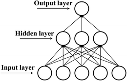
2.3 Methodology of ANN
The three-layer ANN with one input layer, one hidden layer and one output layer was used in this 3D QSPR study. The number needed in the intermediate layer was optimized by an iterative process. The back-propagation algorithm was used to obtain the connection weights, which represents the degree of influence between interconnected neurons. ANN training was accomplished if the error function is minimized below a predefined threshold. The relative importance v of input variable can be obtained by:| | 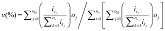 | (2) |
eqn (2) was used with the absolute values of connection weights in order to partition the sum of effects on the output layer. In this equation, nv is the number of input neurons, nH is the number of hidden neurons, oj is the hidden-output layer connection weight values, and ij is the input-hidden connection weight values. It gives the relative importance or distribution of all output weights attributable to the given independent input variables.
2.4 Methodology of SVM
The SVM maps the input vector x onto a very high-dimensional feature space F via a nonlinear mapping Φ and then to perform linear regression in the feature space. Therefore, regression approximation addresses the problem of estimating a function based on a given dataset G = {(xi, di)}li=1 (xi is input vector, di is the desired value). SVM approximates the function in the following form| | 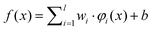 | (3) |
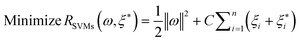
where w is a vector in F, {ϕi(x)}li=l is the set of mappings of input variables, and b is coefficient. w and b are estimated by minimizing the regularized risk function R(C)| | 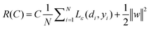 | (4) |
where| | 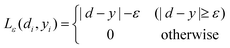 | (5) |
ε is a prescribed parameter.
The first term, 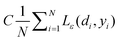 , of function (4) is called empirical error (risk) and it is calculated by the ε-insensitive loss function (5). This sets an ε range so that if predicted result is within the range, the loss is zero, while if predicted point is outside the range, the loss is the difference between the predicted result and the radius ε of the range. C is a penalty parameter, which is a regularized constant to determine the trade-off between training error and model flatness. The second term of the function (4), 1/2‖w‖2, is the regularized term, which will make a function as flat as possible, thus playing role of controlling the function capacity. The introduction of the ξ and ξ* positive slack variables results in eqn (6), to the following constrained function:
| |  | (6) |
in
eqn (6),
i stands for the data sequence, with
i = 1 being the earliest observation. Decision function
(7) takes the form below, after introducing the Lagrange multipliers and exploiting the optimality constraints:
| | 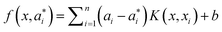 | (7) |
in
eqn (7),
ai and
a*i are the introduced Lagrange multipliers. With the utilization of the Karush–Kuhn–Tucker (KKT) conditions, only a limited number of coefficients will not be zero among
ai and
a*i. The related data points could be referred to as the support vectors. In
eqn (7),
K refers to the kernel function, including the linear, polynomial, splines and radial basis function.
With respect to the support vector regression, the radial basis function (RBF) which is broadly employed is the Gaussian radial basis function (8):
| | 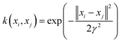 | (8) |
where
γ is the width parameter.
The predictive precision of the models for external validation data were checked by root mean squared error (RMSE) function (9). RMSE is calculated by taking the square root of the squared residuals. Residuals are the differences between predicted values and actual values. Partial residual plots were generated by plotting each independent variable against the residuals. RMSE values were used to quantify the external validation strength of the predictions.
| | 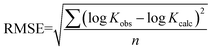 | (9) |
3. Results and discussion
3.1 3D QSPR model development using MLR
In order to construct a high quality 3D QSPR model, MLR analysis was performed on 39 aromatic compounds selected from previous studies. In addition, 13 physicochemical properties, related to aromatic compounds adsorption from aqueous phase, of 3D structure were obtained from Qikprop (Maestro, version 9.2, Schrodinger, LLC, New York, 2011). QSPR models with 3D structure properties were constructed using a forward selection algorithm embedded in the Strike program (Maestro, version 9.2, Schrodinger, LLC, New York, 2011); additionally, 30 aromatic compounds investigated by Xia et al. were used for model validation.40
Because of the moderate size of the dataset, an internal validation method, leave-one-out cross-validation (LOOCV), was applied. This LOOCV approach was used to verify the choice of model. In LOOCV, one observation at a time is removed from the dataset, and the remaining observations are used successively to predict the deleted observation.
As expected, R2 represents the linearity of regression analysis and the extent of consistency between the experimental data and model predictions. The relationship between R2 and dependent parameters in 3D QSPR models is shown in Fig. 2. The program recommends using a dataset with at least five times as many molecules as there are independent descriptors (Schrödinger, LLC, New York, NY, 2011). Since we have 39 compounds in training dataset, we have to fix 7 variables as maximum.41–43 However, the 3D QSPR models did not improve much beyond five descriptors. Therefore, the optimum result obtained by Strike with forward selection algorithm is given by eqn (10).
| | | logKSA∞ = −4.029 + 0.5409 × (logKow) + 0.7504 × (#NandO) + 0.1525 × (#ringatoms)−0.1657 × (dipole) − 0.5888 × (accptHB) | (10) |
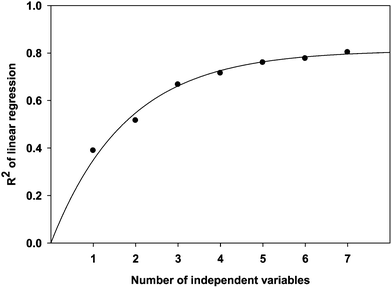 |
| | Fig. 2 Progress in R2 as the number of independent variables increases during the QSPR model development. | |
The five selected parameters that produced the optimum correlation between the predicted and observed relative adsorbabilities were evaluated in the Strike program; the selected parameters (F and P) are shown in Table 4. If 5 < F < 33 and P < 0.05, then the model was construed as significant, and T value associated with each descriptors relating to the significance of the corresponding parameter (Table 4).
Table 4 Parameters of MLR statistics
| Descriptors |
logKow |
Dipole |
AccptHB |
#NandO |
#ringatoms |
|
| T |
4.93 |
2.59 |
3.49 |
5.06 |
4.85 |
|
| F |
|
|
|
|
|
20.9 |
| P |
|
|
|
|
|
2.27 × 10⁻⁹ |
All the descriptors in the above equation are defined in Table 5: logKow is the octanol/water partition coefficient, #NandO is the number of nitrogen and oxygen atoms, #ringatoms is the number of atoms in rings of a ring molecule, dipole is the computed dipole moment of the molecule, and accptHB is estimated number of hydrogen bonds that would be accepted by the solute from water molecule in an aqueous solution.
The values of descriptors for the aromatic compounds in the validation (testing) dataset are shown in Table 3; additionally, the range of values for the compounds in the training dataset was comparable with the range of values for the compounds in the testing dataset (Fig. 3). The predicted values were compared with the experimentally obtained logKSA values, as presented in Fig. 4; the R2 for the validation set was calculated as 0.5093. The following equation is the regression for testing dataset:
| | | logKSA predicted = (0.7112 ± 0.1319) logKSA experimental − 0.7425 | (11) |
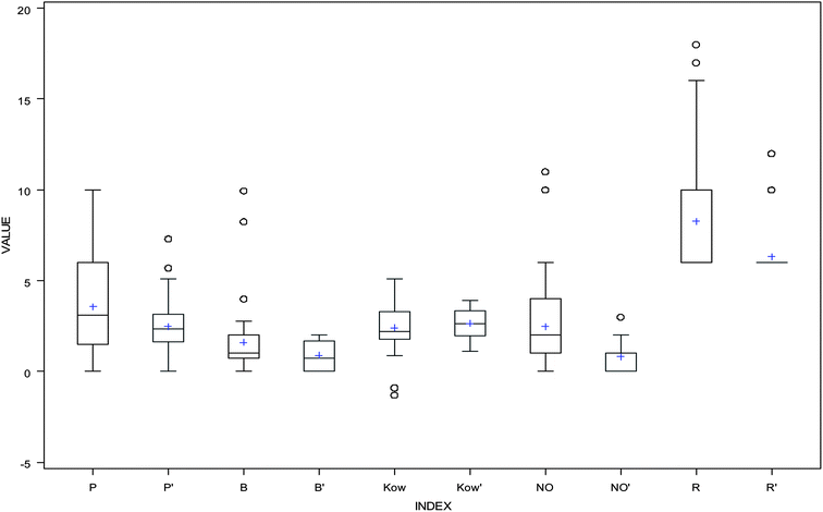 |
| | Fig. 3 Box and whisker plots for the 3D QSPR descriptors: P and P′ represent dipole values in training and testing dataset, B and B′ represent accptHB values in training and testing dataset, Kow and K′ow represent logKow values in training and testing dataset, NO and NO′ represent NandO values in training and testing dataset, and R and R′ represent ringatom values in training and testing dataset. | |
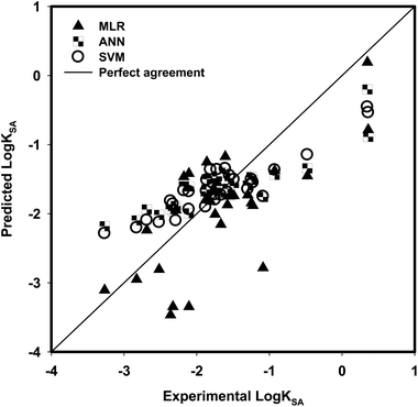 |
| | Fig. 4 Comparison between the experimental logKSA and model predicted logKSA using MLR, ANN and SVM for testing dataset. | |
Based on eqn (10), we can attempt to explain mechanism of adsorption of aromatic compounds by MWCNTs. LogKow represents the hydrophobic properties of aromatic compounds; compounds with large logKow values will tend to participate more easily into a hydrophobic phase than a hydrophilic phase (water phase). Thus, the MWCNTs with hydrophobic surface can adsorb more aromatic compounds with large values of logKow, resulting in large values of logKSA. This is the reason that logKow has a positive significance for prediction of aromatic compounds adsorption by MWCNTs.
For #NandO, in the database of 39 compounds, 34 of them contain nitrogen and oxygen atoms; within these 34 compounds, as the number of nitrogen and oxygen atoms increases, the molecular size of these compounds also increases. These molecules include more hydrophobic groups (–NO2), benzene rings and more branch chains with nitrogen atoms added, and the lengths of branch chains increases. These added properties decrease the solubility of aromatic compounds and increase the adsorption of aromatic compounds onto MWCNTs, which results in the positive correlation of #NandO with the adsorption descriptor.
In terms of #ringatoms, because the selected compounds are aromatic compounds, the number of atoms in rings is related to the number of aromatic ring in the compounds, i.e. a high number of atoms in rings represent more aromatic rings in the compounds. More aromatic rings in an aromatic structure increase the molecule weight/volume and π–π bond of selected aromatic compounds. Therefore, the positive effect of #ringatoms directly decreases the solubility of aromatic compounds and increases the adsorption of aromatic compounds onto MWCNTs.
For dipole, molecules are said to be polar because they possess a permanent dipole moment. A highly polar molecule leads to a large dipole moment. According to “like dissolves like” rule, a molecule with a large dipole moment has more solubility in water, which directly decreases adsorption of aromatic compounds onto MWCNTs in aqueous solution; therefore, a negative correlation of dipole of aromatic compounds adsorbed by MWCNTs was obtained.
Higher accptHB values represent the higher capacity of solute to accept hydrogen bonds from water molecules. In terms of hydration of the solute, strong hydrogen bond accepting ability of solute supports hydration by the strong hydrogen bond donating water (hydrogen bond donor of water is 1.17).44 This favors solubility in water and decreases the tendency of adsorption of aromatic compounds onto MWCNTs.
3.2 3D QSPR models development using ANN
The ANN approach was applied by including the indicators as input neurons in eqn (2) and with the output neuron logKSA. The ANN structure was optimized by considering the statistical parameters of the regression between the experimental and predicted logKSA values and the training time. The final structure was composed of three neurons in the hidden layer and hyperbolic tangent functions as transfer function (Fig. 5).
 |
| | Fig. 5 Structure of artificial neural network. | |
The 39 aromatic compounds in the training dataset and the same subset of descriptors with MLR were used to build the ANN model; then, in the testing step, the 30 aromatic compounds were used to validate the generated ANN model. Fig. 4 presents the predicted logKSA values as a function of experimental logKSA values. The following equation is the regression for testing dataset:
| | | logKSA predicted = (0.4126 ± 0.04104) logKSA experimental − 0.9173 | (12) |
In the complicated nonlinear relationships between model inputs and outputs, it is difficult to know which of the five physical properties in the input layer significantly influences the simulation results. As well, the R2 for predicting aromatic compounds adsorption coefficients in the ANN for each neuron is hard to describe. The integrated result of ANN in this study has outperformed the multi-regression, which could be the reason the neural network method has better predicted the adsorption of aromatic compounds onto MWNTs. Therefore, to predict reasonable estimates for the adsorption of aromatic compounds by MWCNTs, ANN with suitable structure may be useful tools.
3.3 3D QSPR models development using SVM
After the development of 3D QSPR models using MLR and ANN, SVM was used to build a third prediction model. The LOOCV method implied in SVM was used to perform parameter selection. Similar to other multivariate statistical models, the performances of SVM for regression depend on the combination of several parameters, such as the kernel function type, the capacity parameters C, ε of the ε-insensitive loss function and its corresponding parameters. The 39 aromatic compounds in the training dataset and the same subset of descriptors with MLR and ANN were used to build SVM model; additionally, the same 30 aromatic compounds were used to validate the generated SVM model. The predicted logKSA values as a function of experimental logKSA values were presented in Fig. 4 and eqn (13) presents the regression for testing dataset.| | | logKSA predicted = (0.4679 ± 0.04) logKSA experimental − 0.8342 | (13) |
The corresponding parameter, i.e. γ of the kernel function (eqn (8)), has a very close relation with the SVM performance and training time, and significantly influence the number of support vectors. Regarding γ, it controls the amplitude of the RBF function and accordingly controls the SVM generalization ability. With respect to the capacity parameter C (eqn (6)), it controls the trade-off between the margin maximization and the training error minimization. Low value of C will place insufficient stress on fitting the training data, and high value of C will make algorithm over-fit the training data. The ε of the ε-insensitive parameters was investigated. The ε-insensitive parameter can prevent the entire training set from meeting boundary conditions, which will provide the sparsity possibility in the dual formulation solution. The optimum ε value is strongly affected by the noise type present in the data; however, the noise type is usually unknown. As a consequence, the best choices regarding the γ, ε, and C values were 0.73, 3 and 0.16 for the optimal model; the predicted results of the optimal SVM were shown in Fig. 4.
For 30 testing aromatic compounds, the experimental and predicted logKSA values in three algorithms are listed in Table 6. Fig. 4 exhibits the experimental versus predicted values for the testing sets with the SVM method. The RMSE value of the SVM model for the testing data set was lower than those of the MLR and ANN models (Table 6); however, the R2 given by the SVM model was higher than those of the MLR and ANN models (Table 6). Results in Table 6 confirm the better prediction ability of SVM > ANN > MLR to represent the adsorption data, indicated by a higher R2 and lower RMSE when the test aromatic compounds are included in the testing database. Compared with the results obtained from MLR and ANN, SVM provides the most satisfactory results. The optimized values of γ, ε, and C that were used in SVM development gave a reason why SVM provides better prediction.
Table 5 Descriptors and properties generated by QikProp used for QSPR model development
| Descriptor/property |
Explanation |
| MW |
Molecular weight of the molecule |
| SASA |
Total solvent accessible surface area in square angstroms |
| FOSA |
Hydrophobic component of the SASA (saturated carbon and attached hydrogen) |
| FISA |
Hydrophilic component of the SASA (SASA on N, O, and H on heteroatoms) |
| PISA |
π (carbon and attached hydrogen) component of the SASA |
| WPSA |
Weakly polar component of the SASA (halogens, P, and S) |
| PSA |
Van der Waals surface area of polar nitrogen and oxygen atoms |
| DonorHB |
Estimated number of hydrogen bonds that would be donated by the solute to water molecules in an aqueous solution |
| AccptHB |
Estimated number of hydrogen bonds that would be accepted by the solute from water molecules in an aqueous solution |
| Dipole |
Dipole moment of the molecule |
| #NandO |
Number of nitrogen and oxygen atoms |
| #ringatoms |
Number of atoms in rings |
| #nonHatm |
Number of heavy atoms (nonhydrogen atoms) |
| logKow |
Octanol/water partition coefficient |
Table 6 Comparison of the predictive ability of MLR, ANN and SVM
| No. |
Compounds |
Experimental value (logKSA) |
Predicted value by MLR |
Predicted value by ANN |
Predicted value by SVM |
| 1 |
Acetophenone |
−2.11 |
−3.34 |
−1.99 |
−1.93 |
| 2 |
Azobenzene |
0.35 |
0.19 |
−0.20 |
−0.45 |
| 3 |
Benzonitrile |
−2.33 |
−3.34 |
−1.96 |
−1.86 |
| 4 |
Benzyl alcohol |
−3.27 |
−3.10 |
−2.18 |
−2.28 |
| 5 |
Bromobenzene |
−1.87 |
−1.78 |
−1.65 |
−1.67 |
| 6 |
3-Bromophenol |
−1.58 |
−1.87 |
−1.63 |
−1.69 |
| 7 |
4-Chloroacetophenone |
−1.09 |
−2.78 |
−1.75 |
−1.75 |
| 8 |
4-Chloroanisole |
−1.30 |
−1.73 |
−1.59 |
−1.64 |
| 9 |
2-Chloronaphthalene |
0.36 |
−0.78 |
−0.88 |
−0.53 |
| 10 |
3-Chlorophenol |
−1.75 |
−2.00 |
−1.67 |
−1.72 |
| 11 |
4-Chlorotoluene |
−1.55 |
−1.74 |
−1.52 |
−1.44 |
| 12 |
m-Dichlorobenzene |
−1.72 |
−1.54 |
−1.46 |
−1.36 |
| 13 |
ortho-Dichlorobenzene |
−1.81 |
−1.82 |
−1.48 |
−1.35 |
| 14 |
p-Dichlorobenzene |
−1.86 |
−1.25 |
−1.50 |
−1.51 |
| 15 |
3,5-Dimethylphenol |
−1.88 |
−1.80 |
−1.75 |
−1.89 |
| 16 |
Ethyl benzoate |
−1.23 |
−1.88 |
−1.51 |
−1.54 |
| 17 |
Ethylbenzene |
−2.18 |
−1.47 |
−1.60 |
−1.66 |
| 18 |
4-Ethylphenol |
−1.75 |
−1.67 |
−1.66 |
−1.797 |
| 19 |
4-Fluorophenol |
−2.69 |
−2.23 |
−1.93 |
−2.09 |
| 20 |
Iodobenzene |
−1.49 |
−1.74 |
−1.55 |
−1.50 |
| 21 |
Isophorone |
−2.36 |
−3.46 |
−1.93 |
−1.81 |
| 22 |
Methyl benzoate |
−1.67 |
−2.15 |
−1.69 |
−1.7 |
| 23 |
3-Methylbenzyl alcohol |
−2.52 |
−2.80 |
−2.01 |
−2.12 |
| 24 |
Methyl 2-methylbenzoate |
−1.25 |
−1.84 |
−1.47 |
−1.50 |
| 25 |
1-Methylnaphtalene |
−0.48 |
−1.45 |
−1.34 |
−1.14 |
| 26 |
3-Methylphenol |
−2.29 |
−1.94 |
−1.89 |
−2.09 |
| 27 |
4-Nitrotoluene |
−0.93 |
−1.37 |
−1.43 |
−1.36 |
| 28 |
Propylbenzene |
−1.61 |
−1.17 |
−1.40 |
−1.34 |
| 29 |
Phenylethyl alcohol |
−2.83 |
−2.95 |
−2.09 |
−2.20 |
| 30 |
p-Xylene |
−2.11 |
−1.42 |
−1.60 |
−1.67 |
|
|
RMSE |
|
0.6498 |
0.5016 |
0.4543 |
|
|
R
2
|
|
0.5093 |
0.7829 |
0.8317 |
4. Conclusion
In the present study, three learning approaches (MLR, ANN and SVM) were applied to construct a 3D QSPR model between physicochemical properties of selected aromatic compounds and their adsorption coefficients onto MWCNTs. The developed quantitative relation model indicated the significant relationship between adsorption coefficients and five descriptors. The adsorption of aromatic compounds by MWCNTs is positively related to logKow, #NandO and #ringatoms, and negatively related to dipole and accptHB. The results obtained by SVM were compared with the results obtained by MLR and ANN; the comparison demonstrated that SVM was more powerful in the prediction of the adsorption of aromatic compounds by MWCNTs, followed by ANN and MLR. However, the results of SVM and ANN are close and both are better than the result of MLR, which is because the MLR performs linear regression between logKSA and physicochemical properties. Our results showed that the relation between logKSA and physicochemical properties should be nonlinear. A suitable model with high statistical quality and low prediction errors was eventually derived. The prediction results indicated that there was a good prospect for SVM application to the QSAR model development.
Acknowledgements
This work was supported by a research grant from the National Science Foundation (CBET 0967425). However the manuscript has not been subjected to the peer and policy review of the agency and therefore does not necessarily reflect its views. We thank Dr Sarah Work for her comments on the manuscript of this paper.
References
- K. Yang, W. Wu, Q. Jing, W. Jiang and B. Xing, Environ. Sci. Technol., 2010, 44, 3021–3027 CrossRef CAS PubMed.
- S. Zhang, T. Shao, H. S. Kose and T. Karanfil, Environ. Sci. Technol., 2010, 44, 6377–6383 CrossRef CAS PubMed.
- S. Zhang, T. Shao, S. S. K. Bekaroglu and T. Karanfil, Water Res., 2010, 44, 2067–2074 CrossRef CAS PubMed.
- H. Parham, S. Bates, Y. Xia and Y. Zhu, Carbon, 2013, 54, 215–223 CrossRef CAS PubMed.
- W. Chen, L. Duan and D. Zhu, Environ. Sci. Technol., 2007, 41, 8295–8300 CrossRef CAS.
- C. J. M. Chin, L. C. Shih, H. J. Tsai and T. K. Liu, Carbon, 2007, 45, 1254–1260 CrossRef CAS PubMed.
- S. Zhang, T. Shao and T. Karanfil, Water Res., 2011, 45, 1378–1386 CrossRef CAS PubMed.
- V. K. K. Upadhyayula, S. Deng, M. C. Mitchell and G. B. Smith, Sci. Total Environ., 2009, 408, 1–13 CrossRef CAS PubMed.
- C. Ye, Q. Gong, F. Lu and J. Liang, Acta Phys.-Chim. Sin., 2007, 23, 1321–1324 CrossRef CAS.
- C. Ye, Q.-M. Gong, F.-P. Lu and J. Liang, Sep. Purif. Technol., 2008, 61, 9–14 CrossRef CAS PubMed.
- B. Pan and B. Xing, Environ. Sci. Technol., 2008, 42, 9005–9013 CrossRef CAS.
- X. Wang, Y. Liu, S. Tao and B. Xing, Carbon, 2010, 48, 3721–3728 CrossRef CAS PubMed.
- W. Zhang and S. R. P. Silva, Carbon, 2010, 48, 2063–2071 CrossRef CAS PubMed.
- G. A. Patani and E. J. LaVoie, Chem. Rev., 1996, 96, 3147–3176 CrossRef CAS PubMed.
- J. C. Dearden, Chemom. Intell. Lab. Syst., 1994, 24, 77–87 CrossRef CAS.
- V. Rastija and M. Medic-Saric, Med. Chem. Res., 2009, 18, 579–588 CrossRef CAS.
- H. Lei and S. A. Snyder, Water Res., 2007, 41, 4051–4060 CrossRef CAS PubMed.
- A. M. Redding, F. S. Cannon, S. A. Snyder and B. J. Vanderford, Water Res., 2009, 43, 3849–3861 CrossRef CAS PubMed.
- O. G. Apul, Q. Wang, T. Shao, J. R. Rieck and T. Karanfil, Environ. Sci. Technol., 2013, 47, 2295–2303 CrossRef CAS PubMed.
- K. Dhanachandra Singh, M. Karthikeyan, P. Kirubakaran and S. Nagamani, J. Mol. Graphics, 2011, 30, 186–197 CrossRef CAS PubMed.
- G. Liu and J. Yu, Water Res., 2005, 39, 2048–2055 CrossRef CAS PubMed.
- C. Brasquet, B. Bourges and P. Le Cloirec, Environ. Sci. Technol., 1999, 33, 4226–4231 CrossRef CAS.
- R. M. Aghav, S. Kumar and S. N. Mukherjee, J. Hazard. Mater., 2011, 188, 67–77 CrossRef CAS PubMed.
- R. Guha and P. C. Jurs, J. Chem. Inf. Model., 2005, 45, 800–806 CrossRef CAS PubMed.
- C. Cortes and V. Vapnik, Mach. Learn., 1995, 20, 273–297 Search PubMed.
- H. Liu, X. Yao, R. Zhang, M. Liu, Z. Hu and B. Fan, J. Phys. Chem. B, 2005, 109, 20565–20571 CrossRef CAS PubMed.
- B. Zhao, Z. Zhang and X. Wu, Energy Fuels, 2010, 24, 3066–3071 CrossRef CAS.
- M. H. Fatemi, A. Heidari and M. Ghorbanzade, Bull. Chem. Soc. Jpn., 2010, 83, 1338–1345 CrossRef CAS.
- E. Byvatov, U. Fechner, J. Sadowski and G. Schneider, J. Chem. Inf. Model., 2003, 43, 1882–1889 CrossRef CAS PubMed.
- G. Q. Yu, M. S. Zhang, G. L. Wang and L. Pei, ASCE J. Hydraul. Div., 2012, 43, 105–110 Search PubMed.
- M. Moharrampour, M. K. Ranjbar and A. Mehrabi, Life Sci. J., 2013, 10, 914–919 Search PubMed.
- K. Yang, L. Zhu and B. Xing, Environ. Sci. Technol., 2006, 40, 1855–1861 CrossRef CAS.
- K. Yang, W. Wu, Q. Jing and L. Zhu, Environ. Sci. Technol., 2008, 42, 7931–7936 CrossRef CAS.
- X. Wang, S. Tao and B. Xing, Environ. Sci. Technol., 2009, 43, 6214–6219 CrossRef CAS.
- D. Lin and B. Xing, Environ. Sci. Technol., 2008, 42, 7254–7259 CrossRef CAS.
- H. H. Cho, B. A. Smith, J. D. Wnuk, D. H. Fairbrother and W. P. Ball, Environ. Sci. Technol., 2008, 42, 2899–2905 CrossRef CAS.
- G.-C. Chen, X.-Q. Shan, Y.-S. Wang, B. Wen, Z.-G. Pei, Y.-N. Xie, T. Liu and J. J. Pignatello, Water Res., 2009, 43, 2409–2418 CrossRef CAS PubMed.
- O. G. Apul, T. Shao, S. Zhang and T. Karanfil, Environ. Toxicol. Chem., 2012, 31, 73–78 CrossRef CAS PubMed.
- L. Ji, W. Chen, L. Duan and D. Zhu, Environ. Sci. Technol., 2009, 43, 2322–2327 CrossRef CAS.
- X.-R. Xia, N. A. Monteiro-Riviere and J. E. Riviere, Nat. Nanotechnol., 2010, 5, 671–675 CrossRef CAS PubMed.
-
Suite, LigPrep, version 2.5, Schrödinger, LLC, New York, NY, 2011 Search PubMed.
-
Suite, QikProp, version 3.4, Schrödinger, LLC, New York, NY, 2011 Search PubMed.
-
Suite, Maestro, version 9.2, Schrödinger, LLC, New York, NY, 2011 Search PubMed.
- D. Barrón and J. Barbosa, Anal. Chim. Acta, 2000, 403, 339–347 CrossRef.
- D. Lin and B. Xing, Environ. Sci. Technol., 2008, 42, 5917–5923 CrossRef CAS.
- X. Wang, J. Lu and B. Xing, Environ. Sci. Technol., 2008, 42, 3207–3212 CrossRef CAS.
|
| This journal is © The Royal Society of Chemistry 2013 |
Click here to see how this site uses Cookies. View our privacy policy here.