
 Open Access Article
 This Open Access Article is licensed under a
 Creative Commons Attribution 3.0 Unported Licence
Future environmental impacts of global hydrogen production†
Shijie
Wei
 *a,
Romain
Sacchi
b,
Arnold
Tukker
ac,
Sangwon
Suh
d and
Bernhard
Steubing
a
*a,
Romain
Sacchi
b,
Arnold
Tukker
ac,
Sangwon
Suh
d and
Bernhard
Steubing
a
aInstitute of Environmental Sciences (CML), Leiden University, 2333 CC Leiden, The Netherlands. E-mail: s.j.wei@cml.leidenuniv.nl
bTechnology Assessment Group, Laboratory for Energy Systems Analysis, Paul Scherrer Institute, 5232 Villigen, Switzerland
cThe Netherlands Organization for Applied Scientific Research TNO, The Netherlands
dBren School of Environmental Science and Management, University of California, Santa Barbara, California 93106, USA
First published on 22nd February 2024
Abstract
Low-carbon hydrogen (H2) will likely be essential in achieving climate-neutrality targets by 2050. This paper assesses the future life-cycle environmental impacts of global H2 production considering technical developments, regional feedstock supply, and electricity decarbonization. The analysis includes coal gasification, natural gas steam methane reforming, biomass gasification, and water electrolysis across 15 world regions until 2050. Three scenarios of the International Energy Agency are considered: (1) the Stated Policies Scenario (STEPS), (2) the Announced Pledges Scenario (APS) that entails aspirational goals in addition to stated policies, and (3) the Net Zero Emissions by 2050 Scenario (NZE). Results show the global average greenhouse gas (GHG) emissions per kg of H2 decrease from 14 kg CO2-eq. today to 9–14 kg CO2-eq. in 2030 and 2–12 kg CO2-eq. in 2050 (in NZE/STEPS). Fossil fuel-based technologies have a limited potential for emissions reduction without carbon capture and storage. At the same time, water electrolysis will become less carbon-intensive along with the low-carbon energy transition and can become nearly carbon-neutral by 2050. Although global H2 production volumes are expected to grow four to eight times by 2050, GHG emissions could already peak between 2025 and 2035. However, cumulative GHG emissions between 2020 and 2050 could reach 39 (APS) to 47 (NZE) Gt CO2-eq. The latter corresponds to almost 12% of the remaining carbon budget to meet the 1.5 °C target. This calls for a deeper and faster decarbonization of H2 production. This could be achieved by a more rapid increase in H2 produced via electrolysis and the additional expansion of renewable electricity. Investments in natural gas steam methane reforming with carbon capture and storage, as projected by the IEA, seem risky as this could become the major source of GHG emissions in the future, unless very high capture rates for CCS are assumed, and create a fossil fuel and carbon lock-in. Overall, to minimize climate and other environmental impacts of H2 production, a rapid and significant transition from fossil fuels to electrolysis and renewables accompanied by technological and material innovation is needed.
Broader contextLow-carbon hydrogen could help countries around the world to achieve their net-zero targets. Yet it is still unclear how the hydrogen economy will evolve and which environmental impacts it will cause. Prospective life cycle assessment can help identify solutions that can minimize environmental impacts of hydrogen production along transition scenarios. Guidance should consider existing and emerging technologies, possible temporal and regional differences, and broader socio-economic scenarios that determine the context of these developments. This paper considers both possible developments at the technology level as well as wider economic developments, such as the energy transition, based on shared socioeconomic pathways (SSPs) scenarios used (e.g., in the context of IPCC reports) to quantify the environmental impacts of global hydrogen production until 2050. |
1. Introduction
To limit global temperature increase at the end of this century to 1.5 degrees Celsius (°C) compared to pre-industrial times, it is necessary to achieve carbon neutrality in 2050 or earlier.1 Hydrogen (H2) can be essential in transitioning to a net-zero energy system,2 especially in the transport and heavy industry sectors.2,3 As a result, H2 demand could increase six-fold by 2050.2 Currently, H2 is mainly produced as industrial feedstock from fossil fuels, primarily via coal gasification (CG) and steam reforming of natural gas (NG SMR).4 Low-carbon alternatives that could cover the future demand for H2 include water electrolysis using low-carbon electricity,5 biomass gasification (BG), and fossil fuels coupled with carbon capture and storage (CCS). However, these technologies represent less than one percent of the global market today.2,4 Further, low-carbon H2 technologies may have environmental trade-offs that are not yet fully understood.6,7Understanding the environmental impacts of emerging H2 technologies is essential for adequately developing a roadmap and identifying an environmentally optimal trajectory to deploy H2 technologies. A life-cycle perspective is required to obtain a complete picture of the environmental impacts of H2 production. Life-cycle assessment (LCA) is suitable for assessing products and services’ environmental performance throughout their life-cycle.8
Several LCA studies on H2 production are available, e.g., Bhandari et al.,9 Siddiqui et al.,10 Palmer et al.,11 and Bauer et al.12 These studies show that H2 produced from water electrolysis powered by renewable electricity, biomass, and fossil fuel coupled with CCS leads to a substantial reduction in greenhouse gas (GHG) emissions compared with traditional production pathways but are also not free from environmental burdens. Considering that clean H2 technology is an emerging solution within the energy landscape, several studies used prospective approaches in such LCAs. By incorporating expectations about process efficiency improvement, changes in properties of electrolyzers such as lifespan and material requirements, and possible decarbonization of the electricity mix, the prospective environmental impacts of H2 production were assessed for various regions and countries. For example, Valente et al.13 calculated the future carbon footprint of H2 produced from NG SMR, BG, and water electrolysis by alkaline electrolyzers (AE) powered by grid and wind electricity in 2030 and 2050 in Spain. Delpierre et al.14 compared the environmental impacts of wind power-based H2 production by AE and proton exchange membrane electrolyzers (PEM) in the Netherlands in 2019 and 2050. Using a scenario generated by integrated assessment models (IAMs), coherently incorporating future dynamics of the energy-economy-land-climate system, Lamers et al.15 quantified the environmental impacts of grid-coupled H2 production by PEM and solid oxide electrolysis cell (SOEC) technology in the USA from 2020 to 2100.
Existing studies mainly focus on a limited number of H2 production technologies in a single region, hindering a complete understanding of future environmental impacts across time and regions of different types of H2 technologies, precisely when and where H2 technology improvements and electricity decarbonization will likely occur. This paper aims to fill this knowledge gap by conducting an LCA of key H2 production options and evaluating LCA results considering future H2 technology improvements and developments in energy and other sectors. This assessment returns impacts per kg of H2 for several environmental indicators across three development scenarios and 15 world regions. This can help guide H2 technology deployment and minimize its environmental impacts.
The main contributions of this paper are as follows:
(1) The life-cycle environmental impacts of H2 production at the regional and global levels are quantified for the first time with a long-term perspective until 2050. This can provide valuable insights and decision support for H2 technology developers and policymakers.
(2) We integrate the H2 production scenarios into prospective LCA databases using the premise16 framework and make this fully available online‡. This will allow future researchers to use our H2 production scenarios directly for prospective LCA studies.
2. Methods and data
2.1. Goal and scope
Using attributional LCA, this paper aims to assess the environmental impacts caused by key H2 production technologies from 2020 to 2050, using both one kg H2 output and the future global H2 demand as functional unit. Adopting a cradle-to-gate scope, a first functional unit is defined as one kg of gaseous H2 output delivered at the user at a purity greater than 99.8% and 25–30 bar pressure. We further calculate impacts for a second functional unit, defined as total global production, according to scenarios further elaborated below.As shown in Fig. 1, nine technologies are considered: CG, NG SMR, BG with or without CCS, and three variants of water electrolysis (i.e., AE, PEM, and SOEC). We consider energy and material efficiency increases for future development and changes in these technologies’ foreground life cycle inventory (LCI) data (see Section 2.2.1). Next, we model prospective changes in region-specific LCI background data with the IAM model REMIND (Regional Model of Investments and Development),17 particularly for the energy system, using relevant shared socioeconomic pathway (SSP) scenarios. The future production volumes of these H2 technologies until 2050 and associated technology shares are based on data from the International Energy Agency (IEA) in 3 scenarios: the Stated Policies Scenario (STEPS), the Announced Pledges Scenario (APS), and the Net Zero Emissions by 2050 Scenario (NZE) (see Section 2.2.2).2,4,18–20 The detailed approach to the LCA is explained in the following sections.
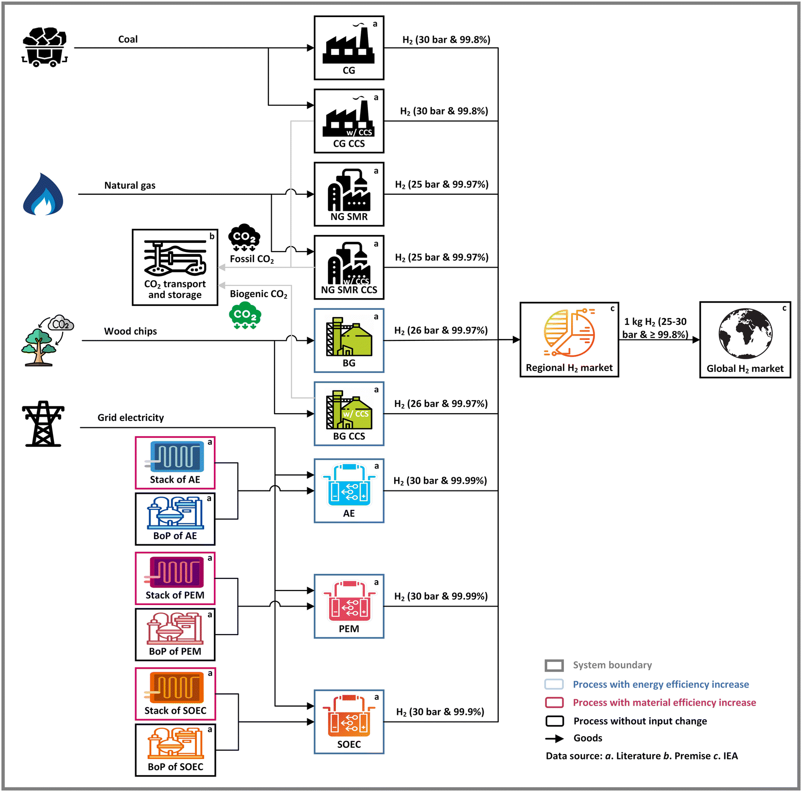 | ||
| Fig. 1 The LCA model of H2 production.§ In this figure, premise is the model of PRospective EnvironMental Impact asSEment.16 IEA = International Energy Agency database and reports.2,4,18–20 | ||
2.2. Life cycle inventories of H2 production
| H2 production technologies | Acronym of H2 technologies | Lifespan of the H2 plant (years) | Net efficiency (lower heating value) (%) | LCI and key parameters source | ||
|---|---|---|---|---|---|---|
| 2020 | 2030 | 2050 | ||||
| a In NG SMR, the tail gas after H2 separation must be burnt with air and additional natural gas in the reformer furnace. When CCS is adopted, the tail gas has less CO2 and a higher heating value. The natural gas demand then decreases. As a result, NG SMR CCS has a higher net efficiency than NG SMR.26 The overall energy efficiency of NG SMR CCS, considering the electricity consumption of CCS, is lower than that of NG SMR. b The electrical efficiency of water electrolysis is the system's efficiency with all utilities (electronics, pumps, safety equipment, infrastructure, etc.) and faradaic losses. For SOEC, electrical efficiency does not include the energy for steam generation. | ||||||
| Coal gasification w/o CCS | CG | 30 | 54.5 | 54.5 | 54.5 | 21–23 |
| Coal gasification w/CCS | CG CCS | 30 | 51.0 | 51.0 | 51.0 | 16 and 22–25 |
| Natural gas steam reforming w/o CCS | NG SMR | 25 | 76.6 | 76.6 | 76.6 | 23 and 26 |
| Natural gas steam reforming w/CCS | NG SMR CCS | 25 | 77.3a | 77.3 | 77.3 | 16, 23, 25 and 26 |
| Biomass gasification w/o CCS | BG | 25 | 54.3 | 57.3 | 64.3 | 27 and 28 |
| Biomass gasification w/CCS | BG CCS | 25 | 54.3 | 57.3 | 64.3 | 16, 25, 27 and 28 |
| Water electrolysis by alkaline electrolyzers | AE | 20 | 67.0 | 68.0 | 75.0 | 23 and 29 |
| Water electrolysis by proton exchange membrane electrolyzers | PEM | 20 | 58.0 | 66.0 | 71.0 | 23 and 29 |
| Water electrolysis by solid oxide electrolysis cell | SOEC | 20 | 78.0b | 81.0 | 84.0 | 23 and 29 |
CG with and without CCS. In the CG route, the pulverized coal is partially oxidized with air or oxygen at high temperatures (800–1300 °C) and pressures of 30–70 bar, producing a syngas mixture composed of H2, carbon monoxide (CO), carbon dioxide (CO2) and small amounts of other gases and particles.30 The raw syngas undergoes a water–gas shift reaction (WGSR) to enhance the H2 yield. The overall reaction is shown in eqn (1).
| C + 2H2O ↔ CO2 + 2H2 | (1) |
After syngas scrubbing and H2 separation using pressure swing adsorption (PSA), waste gases rich in CO2 but also some H2, and CO can generate electricity to offset the plant's energy use or be a co-product of the H2 produced.31 For large sources of CO2 emissions like CG, NG SMR, and BG plants, CCS technology is expected to capture their CO2 from waste gas by various capture technologies, including physical or chemical absorption processes. After compression, captured CO2 is transported by pipeline, ship, rail, or truck and injected into deep geological formations such as saline aquifers or depleted oil and gas reservoirs.32 It is assumed that the captured CO2 can be sequestered underground safely for over 10![[thin space (1/6-em)]](https://www.rsc.org/images/entities/char_2009.gif) 000 years so that it does not contribute to climate change.32,33 The LCI data for CG and CG CCS, including hard coal, electricity, water, and CO2 emissions, is from the National Renewable Energy Laboratory (NREL).21,24 The LCI of infrastructure, waste treatment, and ammonia and hydrogen chloride emissions of CG were supplemented by data from Wokaun et al.22 In the CG process, 3.18 kW h of electricity is produced as a co-product21 and assumed to offset the environmental burdens of electricity from the grid using the substitution method.34,35
000 years so that it does not contribute to climate change.32,33 The LCI data for CG and CG CCS, including hard coal, electricity, water, and CO2 emissions, is from the National Renewable Energy Laboratory (NREL).21,24 The LCI of infrastructure, waste treatment, and ammonia and hydrogen chloride emissions of CG were supplemented by data from Wokaun et al.22 In the CG process, 3.18 kW h of electricity is produced as a co-product21 and assumed to offset the environmental burdens of electricity from the grid using the substitution method.34,35
Selexol solvent is used in the carbon capture technology for CG CCS,24 and its LCI comes from Volkart et al.25 It co-captures CO2 and particulates, but other emissions remain unaffected.36 With a capture rate of 90%, the captured CO2 amounts to 20.39 kg per kg H2, leaving 2.27 kg CO2 per kg H2 uncaptured.24 The electricity consumption for CO2 capture, dehydration, and compression (to 150 bar) is 0.24 kW h per kg CO2.24,37,38 The LCI of CO2 transport and storage and their configurations are from Volkart et al.25 and Sacchi et al.16 CO2 transport by pipeline was conservatively assumed to be over a distance of 400 km.25 Saline aquifers are assumed as CO2 storage sites as they have the largest storage potential.39 A conservative assumption of CO2 sequestration depth of 3 km is considered,40 which is well beyond the 800 meters required to keep the CO2 in a supercritical state.41 The same CO2 transportation and storage configuration is applied to the NG SMR CCS and BG CCS.
NG SMR with and without CCS. In NG SMR, methane reacts with steam using a catalyst at relatively high temperatures (650–1000 °C) and 5–40 bar pressures to produce CO and H2. Like coal gasification, the raw syngas undergoes a WGSR to recover more H2 by reacting CO with steam.42 In the WGSR, a high-temperature water-gas shift reactor is linked to an additional low-temperature one.26 The overall reaction is represented by eqn (2). The excess steam is used for power generation to run the auxiliaries of the plant, and the surplus electricity goes to the grid.26
| CH4 + 2H2O ↔ CO2 + 4H2 | (2) |
There are two sources of CO2 in an SMR plant. One is the oxidation of the carbon in the feedstock during reforming and shift, accounting for 60–72% of the CO2 emissions.26 The other is tail gas combustion from PSA after H2 separation, with air and additional natural gas in the reformer furnace. These CO2 emissions can, in principle, be captured by a pre-combustion and a post-combustion CCS plant, respectively. But in NG SMR CCS, in practice, only a pre-combustion CCS plant is likely to be used, being the most economical option.43 The LCI of NG SMR and NG SMR CCS are from Antonini et al.26 For NG SMR CCS, methyl diethanolamine (MDEA) is the solvent used to capture CO2 with a capture rate of 90% (note that this excludes emissions from the reformer furnace).26 The electricity consumption of CO2 capture, dehydration, and compression is 0.18 kW h per kg CO2.26,37,38
BG with and without CCS. Like CG, BG consists of steam gasification, gas cleaning, WGSR, and H2 separation via PSA.31 It takes place at temperatures of 500–1400 °C and up to 33 bar pressures.44 The BG uses an entrained flow gasifier as the gasification technology.27 The overall reaction is represented by eqn (3). Except for mature technologies such as CG and NG SMR, other emerging H2 production technologies are expected to improve efficiency. With the net efficiency increases, the wood chips input, corresponding CO2 emissions, and required demand for CCS decrease. Except for the 5.5% of carbon losses during the pretreatment and gas cleanup,27 the rest of the CO2 emissions are assumed to be captured with a capture rate of 90% by the MDEA solvent. The LCI of the MDEA and water use for the CCS system are not given in Antonini et al.27 and are sourced from Hospital-Benito et al.45 The electricity requirement for CO2 capture, dehydration, and compression is 0.19 kW h per kg CO2.27,37,38 The biogenic CO2 source coupled with CCS provides negative emissions.46 For BG with and without CCS, wood chips are sourced from sustainably managed forests.27
| Biomass + H2O ↔ H2 + CO + CO2 + CH4 + Tar + Char | (3) |
Water electrolysis. Water electrolysis is a promising technology that utilizes low-carbon electricity to split water into H2 and oxygen, as represented by eqn (4).47 Water electrolysis can be subdivided into three electrolyzer technology types: AE, PEM, and SOEC. AE employing an aqueous potassium hydroxide solution is the most commercially mature technology and operates at 60–90 °C.48 PEM offers higher current densities, dynamic operation, and compact system design, but is also more expensive than AE and operates at lower temperatures of 50–100 °C.48,49 Commercial rollout of PEM is expected in the next ten years at the megawatt-scale.50,51 SOEC is an emerging technology that is still in the research and development stage.52,53 It operates at high temperatures of 600–900 °C and could have the highest electrical efficiency among three main electrolyzers. If the required heat can be supplied from another exothermic process, e.g. ammonia production, this heat can be used instead of a dedicated heat supply to convert water into steam.29
All electrolyzers consists of stacks in series, where water electrolysis takes place, and a balance of plant (BoP). The BoP consists of all the supporting components and auxiliary systems, such as gas conditioning units, water and electricity feedstock conditioning units, and piping and instrumentation required to operate the electrolyzer.54,55
| 2H2O ↔ 2H2 + O2 | (4) |
We use the initial LCI for water electrolysis, including the stack and BoP production of AE, PEM, and SOEC from Gerloff29 and Bareiß et al.56 Nafion, a sulfonated tetrafluoroethylene-based fluoropolymer-copolymer, is considered as membrane material for the PEM stack. It is assumed to be composed entirely of tetrafluoroethylene in Gerloff's research.29 According to Simons et al.,57 we further decompose 16 kg Nafion required for 1 MW PEM stack into 9.2 kg tetrafluoroethylene and 6.8 kg sulfuric acid. We further complete the LCI of the land footprint of electrolyzers, with 135 m2 MW−1, 105 m2 MW−1, and 55 m2 MW−1 for AE, PEM, and SOEC, respectively,58,59 which is lacking in the initial LCI. In Gerloff,29 feedstock water use per kg H2 was set as 9 kg according to the stoichiometric coefficients. But in practice, more feedstock water should be used due to losses, up to 12 kg per kg H2.60 This value is used in our inventory. The cooling water demands per kg H2 are 0.088 m3 for AE and PEM, and 0.645 m3 for SOEC.29 The electricity input in these three types of water electrolysis technologies is adjusted according to their respective efficiencies in 2020, as reported by IEA.23 As the electrolyzers’ efficiencies improve, electricity demand for producing a unit of H2 reduces. In addition, the delivery purity and pressure of the H2 from AE and SOEC are not apparent in Gerloff,29 we further clarify this point in the ESI† Section 1.
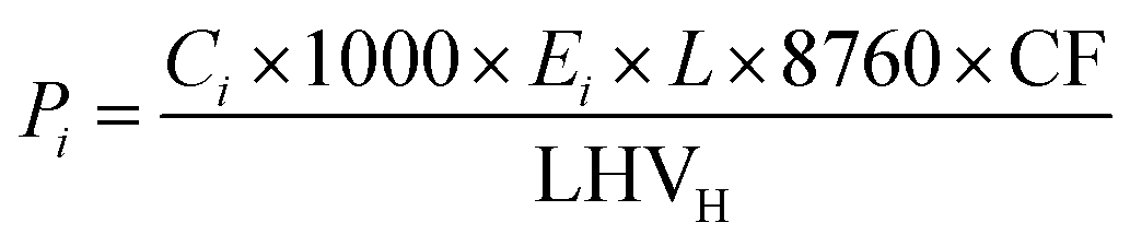
While in the case of CG/NG SMR/BG, the environmental impacts are driven by fuel consumption and their direct emissions, the electrolyzer infrastructure is further considered due to its potentially significant impacts. To consider the plant infrastructure in the LCI, we first need to relate the cumulative production of H2 over the plant's lifetime (assumed to be 20 years29) to the infrastructure requirements. The production amount of H2 during a 20-year lifetime can be calculated as eqn (5):
 | (5) |
As the functional unit is 1 kg H2, we calculate the electrolyzer (1 MW) input and divide it by the H2 production amount over 20 years. The lifetime of the stack is generally shorter than that of BoP. Multiple stack replacements are required during the operation period of the electrolyzer system's whole lifespan.56 In 2020, three stack replacements are required during the 20-year lifetime for AE and PEM, while SOEC needs nine times stack replacements.62 As shown in Table 2, increasing research and development funding and induced production scale-up will lead to an extension of lifetime for stacks.63 Note that the values used in this paper are slightly more conservative than those of the Hydrogen Analysis Production Models (H2A) developed by NREL.64
We also consider likely reductions of material use in the stack production itself due to manufacturing process improvements in the future. The changes in specific material requirements from 2020 to 2050 are shown in Table 3 (see also ESI† Table S20 for an example of how these values are included in the LCI data).
| Materials (kg MW−1) | 2020 | 2050 | Ref. |
|---|---|---|---|
|
a According to Delpierre et al.,14 steel consumption in the electrolyzer stack could decrease. The steel demand decrease in stack production of AE and SOEC is assumed to be the same as that of PEM: 60% from 2020 to 2050. Although the AE is a mature technology, there is a 4365–13095 kg steel consumption range for a 1 MW stack by 2050.14,29 Hence, this assumption seems reasonable.
|
|||
| AE, steela | 20194 |
8078 | 29 and 56 |
| PEM, iridium | 0.75 | 0.03 | 56 |
| PEM, platinum | 0.075 | 0.02 | 56 |
| PEM, titanium | 528 | 35 | 56 |
| PEM, Nafion | 16 | 2 | 56 |
| PEM, activated carbon | 9 | 4.5 | 56 |
| PEM, steel | 100 | 40 | 56 |
| SOEC, steel | 8976 | 3590 | 29 and 56 |
Current H2 production. Although the global H2 production volumes by technology and the H2 production volumes in the 15 IEA regions were available for 2020,4,18 there was no complete disaggregation of H2 production by technology and region. For most regional H2 markets in 2020, the production amounts for H2 from unabated coal and natural gas are collected from the IEA reports,4,19 while the production amounts of H2 production from CCS projects and different types of water electrolysis are obtained from IEA's Hydrogen Production Projects Database.20 However, data gaps for some regions had to be filled based on information from other sources. We refer to the detailed description of assumptions and data sources in Section 2.1 of the ESI.†
Future H2 production. For the future, we base our analysis on the STEPS, APS, and NZE scenarios for both the expected increase in H2 production volumes and the technologies’ market shares. The STEPS scenario considers existing and upcoming policies but does not foresee a drastic change in H2 production.65 This scenario corresponds to a global mean surface temperature (GMST) rise compared to pre-industrial levels of around 2.5 °C by 2100.18 The APS and NZE scenarios foresee a significant rise in H2 production. APS is a scenario that assumes that all climate commitments made by governments worldwide, including Nationally Determined Contributions and longer-term net zero targets and targets for access to electricity and clean cooking, will be met in full and on time.65 This scenario will keep the GMST in 2100 at around 1.7 °C.18 The NZE scenario is a normative IEA scenario that shows a pathway for the global energy sector to achieve net zero CO2 emissions by 2050. It assumes a higher pace of innovation in new and emerging technologies, a greater extent to which citizens are able or willing to change behavior, a higher availability of sustainable bioenergy, and a more effective international collaboration.65
Specifically, the global H2 production volume increases from 70 Mt in 2020 to 121 Mt, 263 Mt, and 528 Mt in 2050 in the STEPS, APS, and NZE scenarios, respectively2,4,18 (as shown in Fig. 4) to satisfy the demand for H2 from traditional applications (industry and refining) and new uses (transport, buildings, agriculture, power generation, production of H2-derived fuels and H2 blending in gas grid).2,66 In the STEPS scenario, the increase stems mainly from conventional technologies, such as CG and NG SMR, as well as water electrolysis. There is a shift from conventional technologies to CCS and water electrolysis in the APS and NZE scenarios. Bioenergy-based H2 does not play an important role. Its production volume is only 1.4 Mt in 2050 in the NZE scenario.2 For this study, we estimate the future H2 production mix in 15 IEA regions. We extrapolate the current production mix per region, as discussed above, with some adjustments based on IEA and literature data to meet the IEA global totals. These calculations and assumptions are provided in Section 2.2 of the ESI.† Although REMIND also models the production and use of H2, we do not use its projections for two reasons. First, its H2 production volume in 2020 is minimal and not in line with actual production (i.e., around 3 Mt). Second, REMIND limits the use of H2 to the industry, building, and transport sectors,17 which is not as comprehensive as the IEA scenarios.
The LCI background databases are derived from a combination of the ecoinvent v3.8 (system model “Allocation, cut-off by classification”) database72 and the REMIND model17 (among the five IAM used for deriving marker scenarios of SSPs69) by using the open-source Python library premise v1.5.8.16 In these databases, the electricity sector by region is updated. Updating the electricity inventories implies an alignment of regional electricity production mixes and efficiencies for several electricity production technologies, including CCS technologies and photovoltaic panels.15,16 To match the market data provided by the IEA to the regional disaggregation of the REMIND-based prospective LCI background data from premise, a regional correspondence is established (the matching of regions and a list of countries associated with these regions can be found in Section 3 in the ESI†). Process inputs from the same region as the H2 production region are paired based on this correspondence, if available, the rest of the world or the global level is used otherwise.
2.3. Life cycle impact assessment
Characterization factors provided by the IPCC's Fifth Assessment Report are used to quantify global warming potentials with a time horizon of 100 years.73 To those we add characterization factors for the uptake and release of biogenic CO2 (i.e., −1 and +1, respectively) and H2 emissions (i.e., +11), needed to correctly consider negative emissions technologies, such as bioenergy with CCS, and H2 leakages, as H2 can act as an indirect greenhouse gas.74 15 other environmental indicators are quantified by the method of EF v3.0:75 acidification (mol H+-eq.), ecotoxicity: freshwater (CTUe), resource use: energy carriers (MJ), eutrophication: aquatic freshwater (kg P-eq.), eutrophication: aquatic marine (kg N-eq.), eutrophication: terrestrial (mol N-eq.), human toxicity: cancer effects (CTUh), human toxicity: non-cancer effects (CTUh), ionizing radiation: human health (kBq U235), land use (dimensionless), resource use: minerals and metals (kg Sb-eq.), ozone depletion (kg CFC-11-eq.), particulate matter (disease incidences), photochemical ozone formation (kg NMVOC-eq.) and water use (kg world eq. deprived). Life cycle impact assessment results are calculated with the Activity Browser.76 The superstructure approach77 is used to handle LCA calculations with multiple foreground scenarios and prospective LCI background databases (representing the different REMIND scenarios across time).
3. Results and discussion
3.1. Prospective GHG emissions of H2 production pathways
Fig. 2 shows the GHG emissions of various H2 technologies per kg H2 produced in China, the USA, and the EU from 2020 to 2030 and 2050. The figure also shows the contributions of different processes to the total global warming potential. The GHG emissions of CG and NG SMR hardly change and increase somewhat over time in China and the USA. One reason for this is that co-produced electricity provides fewer substitution benefits in the future due to a largely decarbonized electricity mix. When CG is coupled with CCS, the overall GHG emissions reduction in 2020 is 59%, 75%, and 73% in China, the USA, and the EU, mainly due to the different regional GHG emissions of coal supply. China has higher GHG emissions per unit of H2 produced from CG CCS, decreasing from 9.7 kg CO2-eq. in 2020 to 7.5 kg CO2-eq. in 2050 due to its carbon-intensive coal supply, which is mainly induced by the methane emissions in the mine operation. NG SMR with CCS roughly halves the GHG emissions across all analyzed years. However, it should be noted that GHG emissions of natural gas-based H2 production are sensitive to upstream fugitive methane leakage rates.78 For CG and NG SMR, increasing the CO2 capture rate and reducing the GHG emissions of coal and natural gas supply are likely the most promising routes to further decarbonization.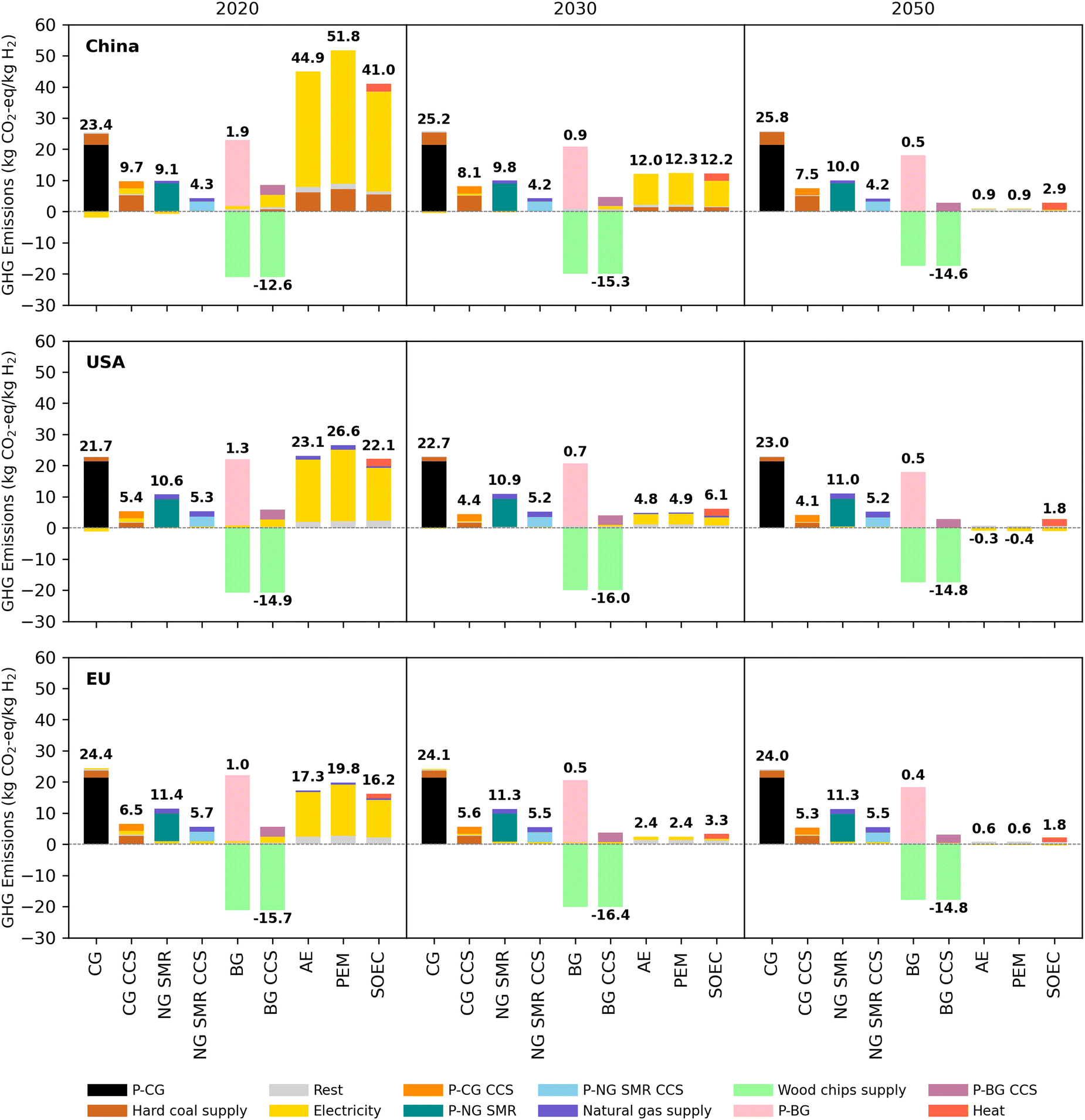 | ||
| Fig. 2 Contribution analysis of GHG emissions of one kg H2 production by different technologies in the NZE scenario. In this figure, the prefix P stands for the process itself, CG = coal gasification, NG SMR = steam methane reforming of natural gas, BG = biomass gasification, CCS = carbon capture and storage AE = alkaline electrolyzer, PEM = proton exchange membrane electrolyzer, and SOEC = solid oxide electrolysis cell. In water electrolysis, the coal and natural gas supply are part of the electricity component. For CG and NG SMR, the negative GHG emissions can be generated by electricity co-produced in the H2 production process when it is assumed to go to the grid. For water electrolysis, the expansion of the bioenergy with CCS in the grid electricity can bring negative emissions. | ||
BG is emphasized among various potential bioenergy-based production routes as it has a high technology readiness level and conversion efficiency.79 Assuming sustainably managed biomass resources, BG is almost carbon-neutral. A variety of biomass feedstocks could be used, e.g., harvested wood products, agricultural residues, and other biogenic waste fractions.80 While BG has been modelled from wood chips here, the specific environmental impacts can vary for other production routes. The role of dedicated energy crops should be examined more critically.81 In the short term, the net GHG emissions reduction of BG CCS is limited partially by electricity use. This reduction grows with electricity decarbonization but eventually declines with efficiency improvements in the BG process (less biomass used to produce one unit of H2). While BG with CCS can yield net negative GHG emissions, its role at the global scale is limited by competing biomass uses,82 land availability, and forest regeneration rates.83,84 Further, the GHG emissions reduction potential depends on the capture rate and energy consumption of carbon capture.36 Even under our conservative assumptions, the GHG emissions for transport and storage 1 kg CO2 are minimal (0.02 CO2-eq. currently, and decreasing with electricity decarbonization).
For H2 production by water electrolysis, the coal- and natural gas-dominated grid electricity currently makes it GHG emissions-intensive. By 2050, significant GHG emissions reduction can be achieved, as high as 98%. This is driven by the decarbonization of the electricity system and efficiency improvements. Due to the dominance of these two factors, the contribution of lifetime extension and material demand decrease of the electrolyzers’ stack to the GHG emissions reduction is minimal (less than 1%). The relative contribution of these drivers can be found in the Section 4.1 in ESI.† Compared to the USA and the EU, China experiences the highest GHG emissions reduction for water electrolysis in the future, declining from 45–52 kg CO2-eq. per kg H2 in 2020 to 0.9–2.9 kg CO2-eq. per kg H2 in 2050. This is because China currently has the most carbon-intensive electricity production. Due to the use of bioenergy with CCS in the power sector, the GHG emissions of water electrolysis in the USA could even become slightly negative in 2050. PEM has the lowest efficiency among the three electrolyzer technologies and has the highest GHG emissions per kg of H2 produced. However, with the increasing decarbonization of the electricity mix in the future, the differences in GHG emissions between AE, PEM, and SOEC become smaller. As we have assumed the heat for SOEC to originate from a dedicated heat production, the heat used to produce steam causes SOEC to have the highest GHG emissions by 2050. If SOEC was to use waste heat, for example, when integrated with ammonia production,85 GHG emissions would further decrease.
3.2. Prospective environmental impacts of global H2 production
Decarbonizing global H2 production can lead to co-benefits and trade-offs with other impact categories. Fig. 3 shows the factor change of environmental impacts per kg H2 from the global H2 market in 2030 and 2050 in the three scenarios. In the APS and NZE scenarios, impacts decrease for the following indicators: particulate matter, ozone depletion, and fossil resource depletion. This relates to the energy transition from fossil fuels to renewable electricity, implying a lesser use of fossil fuels and decreased emissions of ozone-depleting gases and fine particles related to their combustion. In the APS, particulate matter emissions increase in the near term due to the slower power transition compared to NZE. In the NZE scenario, ozone depletion slightly increases in the near term due to using a higher share of natural gas-based power and associated emissions of Halons.86 Near-term eutrophication, photochemical ozone formation, ecotoxicity, and acidification impacts rise due to increased electricity use because of water electrolysis. However, these impacts eventually decline as the power mix shifts predominantly to renewables with minimal nitrogen oxides and sulfur oxides emissions. The increase in human toxicity impacts is tied to the expansion of renewables and the associated release of toxic substances in the environment occurring during the extraction of metals needed to produce photovoltaic panels (e.g., silver, lead, and nickel).87–89 The increase in impact from ionizing radiation is driven by uranium mining as the nuclear power supply expands.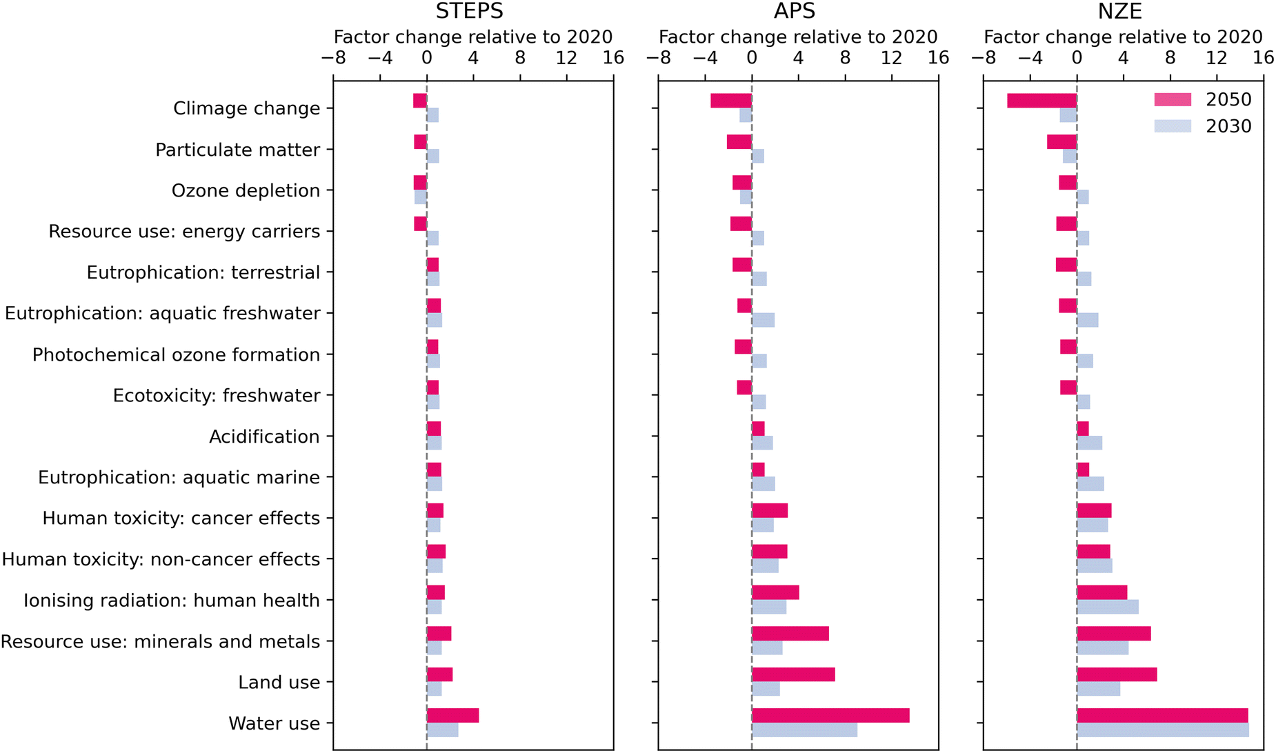 | ||
| Fig. 3 The factor change of future environmental impacts of one kg H2 in the global H2 market in 2030 and 2050 relative to 2020 in the STEPS, APS, and NZE scenarios. Impact categories excluding climate change are from EF v3.0 method. These values are the weighted average values of different regions. Positive and negative values represent that the environmental impacts will increase and decrease many times in the future compared with 2020. Refer to the Tables S29–S44 in ESI† for global and regional absolute values. | ||
Across all scenarios, water, land, and resource use (minerals and metals) increase, driven primarily by the water electrolysis scale-up and corresponding infrastructure construction. In addition, the expansion of renewables is responsible for increased land and metals use, such as neodymium and dysprosium for wind turbines or tellurium and indium for photovoltaic panels.90 Moreover, PEM electrolyzers use platinum and iridium as catalysts to produce H2.91 This technology is regarded as the dominant technology in the future63 and there may be a considerable demand for water electrolysis in different regions. Today, platinum group metals (i.e., platinum, iridium, palladium, ruthenium) are concentrated in five countries: South Africa, Russia, the USA, Zimbabwe, and Canada. South Africa alone produces around 90% of global platinum and 70% of global iridium demand.91,92 An increase in demand for metals may lead to supply risks, especially for rare earth metals.92–94
Although water use has the most significant increase among the other indicators per kg of H2 produced, the overall water use of H2 production is small relative to other sectors, such as the fossil fuel energy production and the agricultural sector.95 In the NZE scenario, the total amount of water used as feedstock for the global H2 production in 2050 is around 4 billion m3. This is lower than global water use of fossil fuel energy production in 2021, 19 billion m3, and far lower than the global agricultural irrigation water use, 1487 billion m3, in 2020.96,97 The selection of the water cooling technology additionally affects water consumption.7,98,99 In a wet cooling tower, around 1% of water flow evaporates into the atmosphere. In a once-through cooling system, the withdrawn water is returned, albeit at a higher temperature, potentially affecting aquatic ecosystems.100 While water use at the global scale should not be a limiting factor for electrolysis, availability could be a limiting factor in specific regions. In locations near the sea, using seawater directly or via desalination could be an alternative to using freshwater.95,101
It should be pointed out that most of the data used in this study (including the scenario data from REMIND and the IEA) was developed with a perspective on GHG emissions. This means that data for impact categories not directly linked to climate change and the energy transition should not be over-interpreted. For example, technological advancements and environmental improvement measures in metal mining or water management that could reduce impacts in other categories, such as human toxicity or water use, are not accounted for. Our findings for other impact categories could thus be overestimations and should rather be seen in the light of highlighting areas for potential improvements.
3.3. Prospective GHG emissions at regional and global levels
Global annual production volumes of H2 increase from about 70 Mt per year in 2020 to 121, 263, and 528 Mt in 2050 in the STEPS, APS, and NZE scenarios, respectively (Fig. 4). This corresponds to an increase by a factor 1.7, 3.8, and 7.5. Global GHG emissions of H2 production are expected to first increase in all scenarios, but then to reduce again in the APS and NZE scenarios, reaching similar emission levels as in 2020, despite much higher H2 production volumes. In the STEPS scenario there is hardly any change in the technology mix and emissions are dominated by unabated fossil fuel-based H2 production. In the APS and NZE scenarios CG and NG SMR without CCS decrease and there is a substantial increase of H2 production via water electrolysis (167 Mt and 321 Mt by 2050) and NG SMR CCS (55 Mt and 190 Mt by 2050). While GHG emissions from water electrolysis strongly decrease with the increasing share of renewable power in the electricity mix, the emissions from fossil fuel-based H2 production are not decarbonized to the same extent. In the NZE scenario, it is expected that after 2040, most H2 production GHG emissions will come from NG SMR CCS. By 2050, annual GHG emissions from NG SMR CCS are projected to be 0.92 Gt, making up 77% of all H2 production related GHG emissions. A further reduction of NG SMR CCS related emissions may be possible if higher CO2 capture rates and lower energy consumption can be achieved.102,103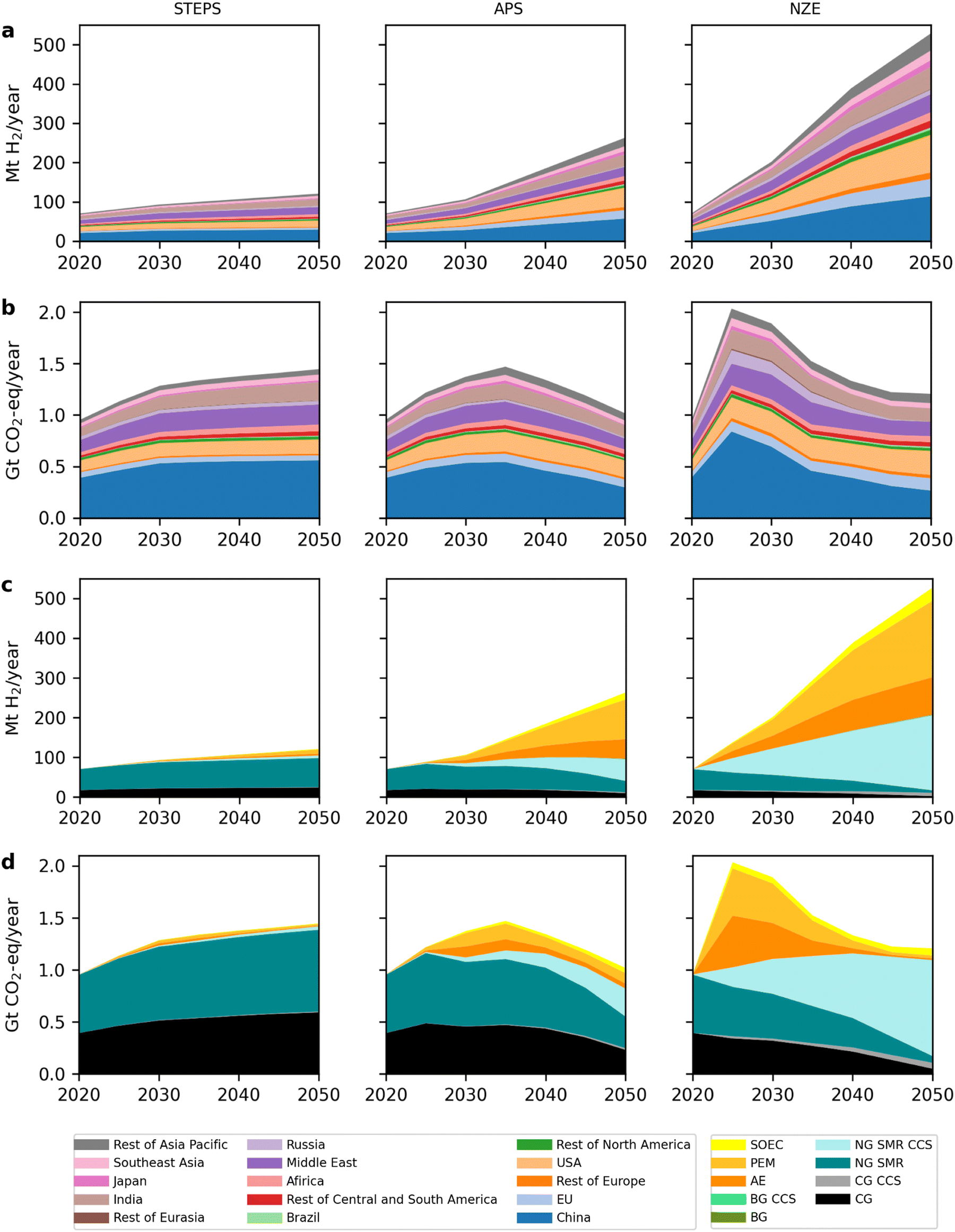 | ||
| Fig. 4 In three scenarios, the global H2 production and annual GHG emissions by region and technology from 2020 to 2050. (a) and (b) Show the H2 production volumes and annual GHG emissions in 15 regions. (c) and (d) Show H2 production volumes and annual GHG emissions of nine technologies. CG = coal gasification, NG SMR = steam methane reforming of natural gas, BG = biomass gasification, CCS = carbon capture and storage, AE = alkaline electrolyzer, PEM = proton exchange membrane electrolyzer, and SOEC = solid oxide electrolysis cell. The water electrolysis is coupled with grid electricity. Although BG CCS has negative emissions, its final contrition is very small because of its limited adoption. | ||
Across all scenarios, China, the USA, India, the Middle East, and the EU are the key producing regions of H2, accounting for roughly 70% of the global aggregated H2 production volume. China will likely remain the largest producer of H2, increasing H2 production from 20 Mt in 2020 to 30–114 Mt in 2050. Currently, most H2 in China is produced from CG, resulting in a high GHG emissions of 19.1 kg CO2-eq. per kg H2 produced in 2020 (Fig. 5). This is not expected to change substantially in the STEPS scenario. In the APS and NZE scenarios, GHG emissions per kg of H2 reduce to 5.2 and 2.4 kg CO2-eq., respectively, due to a shift towards NG SMR CCS and water electrolysis. This leads to a reduction of China's annual GHG emissions from H2 production in 2050 in the APS and NZE scenarios of 0.30 Gt and 0.27 Gt, respectively, compared to 0.39 Gt in 2020.
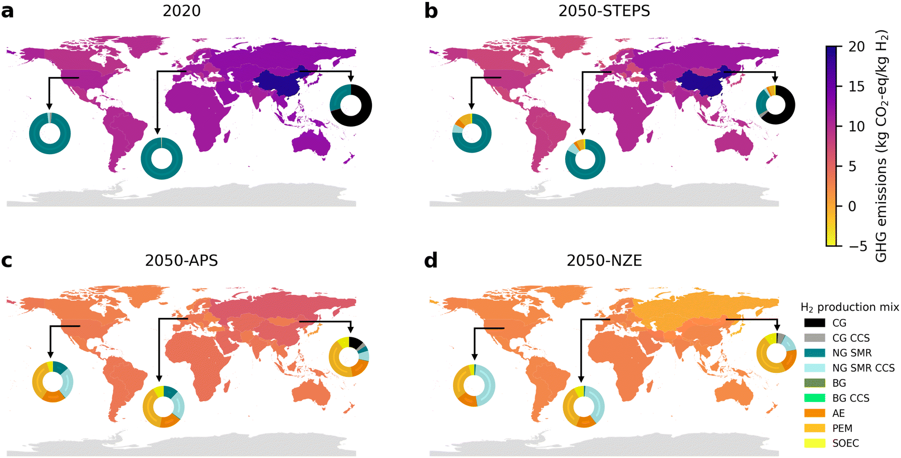 | ||
| Fig. 5 GHG emissions of one kg H2 of regional markets in 2020 and 2050. (a) Shows GHG emissions of per kg H2 from 15 regional H2 market, as well as market share of different H2 technologies in China, the USA and the EU in 2020. (b)–(d) show these values in 2050 in three scenarios. In the legend of H2 production mix, CG = coal gasification, NG SMR = steam methane reforming of natural, BG = biomass gasification, CCS = carbon capture and storage, AE = alkaline electrolyzer, PEM = proton exchange membrane electrolyzer and SOEC = solid oxide electrolysis cell. There is no data for the Antarctic. | ||
The USA and the EU are expected to increase their H2 production from 10 Mt and 5 Mt in 2020 to 16–96 Mt and 5–44 Mt in 2050, respectively. Currently, their H2 production is mostly done via NG SMR, resulting in 10.4 and 11.4 kg CO2-eq. per kg of H2, respectively. These numbers improve to 8.8, 3.4, and 2.4 kg CO2-eq. in the USA and 9.9, 3.6, and 2.7 kg CO2-eq. in the EU by 2050 for the STEPS, APS and NZE scenarios. The larger improvement in the APS and NZE scenarios is driven by the transition to water electrolysis and NG SMR CCS. Compared to 2020 levels (0.10 Gt for the USA and 0.05 Gt for the EU), annual GHG emissions in 2050 increase to 0.16 Gt and 0.23 Gt in the USA and 0.08 Gt and 0.12 Gt in the EU, in the APS and NZE scenarios, respectively.
3.4. Cumulative climate change impacts of H2 production in the future
To understand the impact of H2 production at a large scale on the global carbon budget, we quantify the cumulative GHG emissions of H2 production from 2020 to 2050.104Fig. 6 shows that in 2020, H2 production emitted 0.95 Gt GHG globally.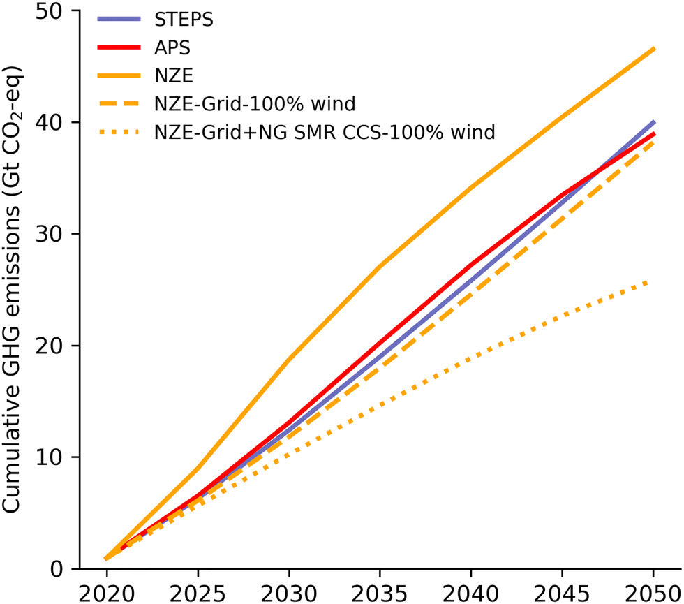 | ||
| Fig. 6 The cumulative GHG emissions of global H2 production from 2020 to 2050 in three scenarios. | ||
Between 2020 and 2050, cumulative GHG emissions from H2 production are projected at 40 Gt (STEPS), 39 Gt (APS), and 47 Gt (NZE). Despite APS producing four times more H2 by 2050 than 2020, its emissions are slightly lower than STEPS. The NZE scenario sees a 16% emissions increase compared to the STEPS, but also octuples H2 production.
Research has shown that the remaining carbon budget for limiting global warming to 1.5 °C with 67% certainty between 2020 and 2050 is about 400 (± 220) Gt CO2-eq.105 Taking 400 Gt as a basis, the 47 Gt CO2-eq. of the NZE scenario amount to 12% of the residual carbon budget (see Section 4.2 in ESI† for regional contributions). This is a very large figure and a faster decarbonization would certainly be desirable.
In the NZE scenario, CG (with and without CCS) contributes 9 Gt (1 Gt and 8 Gt), NG SMR (with and without CCS) contributes 25 Gt (15 Gt and 10 Gt), and water electrolysis contributes to 13 Gt CO2-eq. One way to decarbonize faster, would be to power electrolysis to a higher extent by renewables. In our study we have assumed that water electrolysis technologies is powered by average grid electricity. If all electrolysis-based H2 production was powered entirely by onshore wind energy, global GHG emissions from H2 production between 2020 and 2050 would be reduced by 2.2%, 9.5%, and 17.9% in the STEPS, APS, and NZE scenarios, respectively (see the ESI† Section 4.3 for more details). This would save about 8 Gt GHG emissions in the NZE scenario. If NG SMR CCS was to be replaced with water electrolysis powered by 100% onshore wind, the overall GHG emissions in the NZE scenario between 2020 and 2050 could be reduced by as much as 12 Gt (26.5)%. Together, although somewhat hypothetical, the transition to fully renewable-powered water electrolysis and replacement of NG SMR CCS by the latter could save up to 20 Gt CO2-eq. emissions and reduce the cumulative emissions in the NZE scenario by 44.4%.
This analysis shows the tremendous importance of this sector and the need to achieve further GHG emission reductions, if possible beyond that of the NZE scenario. While there is not only one solution, our study shows that an effective way of realizing further reductions would be the further replacement of fossil-based technologies (e.g. NG SMR CCS) by water electrolysis with renewable electricity. Our sensitivity analysis does not consider additional infrastructure requirements for storing electricity and H2 and possible inefficiencies of off-grid insular solutions that might be required to supply H2 from renewable electricity only. However, the GHG emissions reduction potential from dedicated renewables depends on our ability to develop the additionality, i.e. the dedicated renewable power generation capacity for H2 production,106,107 faster than projected. It is worth noting that increasing H2 production from electrolysis and renewable electricity implies significant investment. For example, to produce more than 3 Mt of clean H2 per year by 2030, the U.S. Department of Energy has announced 7 billion to support seven regional clean H2 hubs, which is to be met by private sector investments of 40 billion.108 Thus, without significant investments by public and private stakeholders, H2 production may not develop as fast as desired.
4. Conclusions
In this work, we systematically assess the environmental impacts of future H2 production technologies until 2050 at the regional and global levels. The assessment includes important drivers of impacts, such as electricity decarbonization, efficiency improvements, advancements in electrolyzer technology, the use of CCS, and changes in the H2 production mix. The IEA scenarios reflect possible consequences of current policy settings (STEPS), realizing all climate commitments in addition to already implemented policy (APS) and achieving net zero CO2 emissions by 2050 (NZE). Our results can inform policy makers on the potential magnitude of future environmental impacts related to an increasing H2 production and options to reduce them further. Our study also provides GHG emission intensities (and the underlying LCI data) of current and future H2 production technologies that can be used to assess the GHG emissions mitigation potential of H2 in different sectors. Our main conclusions are the following:H2 production needs to shift away from fossil fuels
Water electrolysis will have the steepest decrease in GHG emissions per kg H2 output between 2020 and 2050, mainly driven by electricity decarbonization and efficiency improvements. Despite variations across regions (i.e., China, the USA, and the EU) due to different renewables deployment strategies, emissions reduce to almost zero in 2050 in the NZE scenario, regardless of the electrolyzer type. In contrast, traditional H2 pathways (i.e., CG and NG SMR) have much higher GHG emissions per kg H2 produced. Even with CCS GHG emissions are considerably higher. In fact, in all analyzed scenarios fossil fuel technologies still dominate climate change impacts by 2050. The investment into additional NG SMR CCS capacities seem questionable from a GHG perspective, as shown in the NZE scenario, and could create a risky fossil fuel lock-in.109 This conclusion is unlikely to change, unless very high capture rates in CCS can be achieved. Given that there is also uncertainty about whether CCS can be deployed at the required scale and locations,110 a shift towards more electrolysis and renewable electricity seems to be a safer, more climate friendly and future-proof option.H2 production related GHG emissions need to be further minimized and avoid the carbon lock-in risk from CCS
Although the development of a H2 economy is being promoted with the aim to reduce GHG emissions in different sectors,111 our analysis shows that in the NZE scenario the production of H2 alone could consume up to 2050 as much as 12% (47 Gt CO2-eq.) of the remaining carbon budget to meet the 1.5 °C target. This is a staggering quantity of GHG emissions and calls for a faster decarbonization than projected in the analyzed scenarios. This is largely due to NG SMR CCS. CCS only can be expected to have an overall capturing efficiency of 64% for NG SMR. Therefore, NG SMR CCS is almost fully responsible for the 1 Gt CO2-eq. per year emitted by 2050 for H2 production. Since the CCS infrastructure is being build up from 2020 and likely will have a significant remaining technical life time, this will lock in additional carbon emissions at this level for years if not decades after 2050. As discussed, the most promising route seems a more rapid transition to electrolysis based H2 production from renewable electricity, which could reduce cumulative GHG emissions by 2050 to 27 Gt (6.8% of the remaining carbon budget). This would, however, require a faster expansion of renewable electricity generation capacities as assumed in our scenarios.Environmental trade-offs should be further examined and minimized
As CCS and water electrolysis rely increasingly on low-carbon electricity, there are likely co-benefits with other indicators such as particulate matter formation, ozone depletion, and fossil resource depletion. Concomitantly, other indicators could worsen, such as water use, land use, resource extraction and human toxicity. This is mainly due to the scale-up of water electrolysis and the use of renewable electricity. While electrolysis will require considerable amounts of water at the global scale, these amounts are small compared to the global use of water for agriculture. However, for certain regions with high water stress, its feasibility should be critically examined.112 Electrolyzers and renewables will require substantial quantities of metals, however, it has also been shown that the energy transition may substantially reduce the overall mining activity.89 As rare earth metals required by PEM are concentrated in specific countries, the supply risk of these metals in some regions should be carefully assessed before promoting this technology. Toxicity and other environmental impacts related to mining and metal production can also be reduced through improved technologies and better management,113,114 which has not been considered here. Further assessments of specific H2 production technologies and related environmental impacts should be conducted to anticipate and minimize undesired trade-offs locally and at the global scale.Further research needs
The leading H2 technologies considered by the IEA are assessed in this paper. In addition, the environmental impacts of other promising technologies, such as photocatalytic water splitting,115,116 should be further assessed. Further research should be done to assess the potential GHG mitigation effects of using H2 in hard-to-abate sectors (like cement, iron and steel and heavy transport, etc.) and related environmental benefits or trade-offs at the global scale.111 The future scenarios for the H2 production and unit process data presented here may serve as a basis for such analyses.Abbreviations
| AE | Alkaline electrolyzers |
| APS | Announced pledges scenario |
| BG | Biomass gasification |
| BG CCS | Biomass gasification with carbon capture and storage |
| BoP | Balance of plant |
| CCS | Carbon capture and storage |
| CG | Coal gasification |
| CG CCS | Coal gasification with carbon capture and storage |
| CO | Carbon monoxide |
| CO2 | Carbon dioxide |
| GHG | Greenhouse gas |
| H2 | Hydrogen |
| H2A | Hydrogen analysis production models |
| IAM | Integrated assessment model |
| IEA | International energy agency |
| IPCC | Intergovernmental panel on climate change |
| LCA | Life-cycle assessment |
| LCI | Life cycle inventory |
| MDEA | Methyl diethanolamine |
| NG SMR | Steam reforming of natural gas |
| NG SMR CCS | Steam reforming of natural gas with carbon capture and storage |
| NZE | Net zero emissions by 2050 scenario |
| PEM | Proton exchange membrane electrolyzers |
| PSA | Pressure swing adsorption |
| REMIND | Regional model of investments and development |
| SOEC | Solid oxide electrolysis cell |
| SSP | Shared socioeconomic pathway |
| STEPS | Stated policies scenario |
| WGSR | Water–gas shift reaction |
Conflicts of interest
There are no conflicts to declare.Acknowledgements
The authors thank Dr Simon Bennett (IEA) for sharing data about H2 production amounts in the future. The authors further thank Dr Vassilis Daioglou (PBL) for the insight of H2 in the IAM model. The authors also thank Maarten van 't Zelfde (CML) for his help with GIS. The authors also thank the anonymous reviewers for their constructive feedback. This work is supported by the China Scholarship Council (Grant No. 202006430008). Dr Romain Sacchi has received financial support via the research project SHELTERED, funded by the Swiss Federal Office of Energy (SFOE).References
- IPCC, Global Warming of 1.5 °C: IPCC Special Report on Impacts of Global Warming of 1.5 °C above Pre-industrial Levels in Context of Strengthening Response to Climate Change, Sustainable Development, and Efforts to Eradicate Poverty, Report 9781009157957, Intergovernmental Panel on Climate Change, Cambridge, 2018.
- IEA, Net Zero by 2050, International Energy Agency, 2021 Search PubMed.
- I. Staffell, D. Scamman, A. Velazquez Abad, P. Balcombe, P. E. Dodds, P. Ekins, N. Shah and K. R. Ward, Energy Environ. Sci., 2019, 12, 463–491 RSC.
- IEA, Global Hydrogen Review 2021, International Energy Agency, Paris, 2021.
- A. Odenweller, F. Ueckerdt, G. F. Nemet, M. Jensterle and G. Luderer, Nat. Energy, 2022, 7, 854–865 CrossRef.
- C. F. Blanco, S. Cucurachi, J. B. Guinée, M. G. Vijver, W. J. G. M. Peijnenburg, R. Trattnig and R. Heijungs, J. Cleaner Prod., 2020, 259, 120968 CrossRef.
- T. Weidner, V. Tulus and G. Guillén-Gosálbez, Int. J. Hydrogen Energy, 2023, 48, 8310–8327 CrossRef CAS.
- J. B. Guinée, R. Heijungs, G. Huppes, A. Zamagni, P. Masoni, R. Buonamici, T. Ekvall and T. Rydberg, Environ. Sci. Technol., 2011, 45, 90–96 CrossRef PubMed.
- R. Bhandari, C. A. Trudewind and P. Zapp, J. Cleaner Prod., 2014, 85, 151–163 CrossRef CAS.
- O. Siddiqui and I. Dincer, Int. J. Hydrogen Energy, 2019, 44, 5773–5786 CrossRef CAS.
- G. Palmer, A. Roberts, A. Hoadley, R. Dargaville and D. Honnery, Energy Environ. Sci., 2021, 14, 5113–5131 RSC.
- C. Bauer, K. Treyer, C. Antonini, J. Bergerson, M. Gazzani, E. Gencer, J. Gibbins, M. Mazzotti, S. T. McCoy, R. McKenna, R. Pietzcker, A. P. Ravikumar, M. C. Romano, F. Ueckerdt, J. Vente and M. van der Spek, Sustainable Energy Fuels, 2022, 6, 66–75 RSC.
- A. Valente, D. Iribarren and J. Dufour, Int. J. Life Cycle Assess., 2017, 22, 346–363 CrossRef CAS.
- M. Delpierre, J. Quist, J. Mertens, A. Prieur-Vernat and S. Cucurachi, J. Cleaner Prod., 2021, 299, 126866 CrossRef CAS.
- P. Lamers, T. Ghosh, S. Upasani, R. Sacchi and V. Daioglou, Environ. Sci. Technol., 2023, 57, 2464–2473 CrossRef CAS PubMed.
- R. Sacchi, T. Terlouw, K. Siala, A. Dirnaichner, C. Bauer, B. Cox, C. Mutel, V. Daioglou and G. Luderer, Renewable Sustainable Energy Rev., 2022, 160, 112311 CrossRef.
- L. Baumstark, N. Bauer, F. Benke, C. Bertram, S. Bi, C. C. Gong, J. P. Dietrich, A. Dirnaichner, A. Giannousakis, J. Hilaire, D. Klein, J. Koch, M. Leimbach, A. Levesque, S. Madeddu, A. Malik, A. Merfort, L. Merfort, A. Odenweller, M. Pehl, R. C. Pietzcker, F. Piontek, S. Rauner, R. Rodrigues, M. Rottoli, F. Schreyer, A. Schultes, B. Soergel, D. Soergel, J. Strefler, F. Ueckerdt, E. Kriegler and G. Luderer, Geosci. Model Dev., 2021, 14, 6571–6603 CrossRef CAS.
- IEA, World Energy Outlook 2022, International Energy Agency, Paris, 2022.
- IEA, Hydrogen in Latin America: From near-term opportunities to large-scale deployment, International Energy Agency, Paris, 2021.
- IEA, Hydrogen Production Projects Database, International Energy Agency, Paris, 2022.
- NREL, Current Hydrogen from Coal without CO2 Capture and Sequestration, https://www.nrel.gov/hydrogen/assets/docs/current-central-coal-without-co2-sequestration-v2-1-1.xls, (accessed 4th May, 2022).
- A. Wokaun and E. Wilhelm, Transition to Hydrogen: Pathways toward Clean Transportation, Cambridge University Press, Cambridge, 2011 Search PubMed.
- IEA, The Future of Hydrogen, International Energy Agency, Paris, 2019.
- NREL, Current Central Hydrogen from Coal with CO2 Capture and Sequestration, https://www.nrel.gov/hydrogen/h2a-production-models.html, (accessed 4th May, 2022).
- K. Volkart, C. Bauer and C. Boulet, Int. J. Greenhouse Gas Control, 2013, 16, 91–106 CrossRef CAS.
- C. Antonini, K. Treyer, A. Streb, M. van der Spek, C. Bauer and M. Mazzotti, Sustainable Energy Fuels, 2020, 4, 2967–2986 RSC.
- C. Antonini, K. Treyer, E. Moioli, C. Bauer, T. J. Schildhauer and M. Mazzotti, Sustainable Energy Fuels, 2021, 5, 2602–2621 RSC.
- DEA, Technology Data for Renewable Fuels, Danish Energy Agency, 2022.
- N. Gerloff, J. Energy Storage, 2021, 43, 102759 CrossRef.
- R. Kothari, D. Buddhi and R. L. Sawhney, Renewable Sustainable Energy Rev., 2008, 12, 553–563 CrossRef CAS.
- F. Mueller-Langer, E. Tzimas, M. Kaltschmitt and S. Peteves, Int. J. Hydrogen Energy, 2007, 32, 3797–3810 CrossRef CAS.
- IPCC, Carbon Dioxide Capture and Storage, Intergovernmental Panel on Climate Change, New York, 2005.
- J. Alcalde, S. Flude, M. Wilkinson, G. Johnson, K. Edlmann, C. E. Bond, V. Scott, S. M. V. Gilfillan, X. Ogaya and R. S. Haszeldine, Nat. Commun., 2018, 9, 2201 CrossRef PubMed.
- R. Heijungs, K. Allacker, E. Benetto, M. Brandão, J. Guinée, S. Schaubroeck, T. Schaubroeck and A. Zamagni, Front. Sustainability, 2021, 2 Search PubMed.
- Á. Galán-Martín, V. Tulus, I. Díaz, C. Pozo, J. Pérez-Ramírez and G. Guillén-Gosálbez, One Earth, 2021, 4, 565–583 CrossRef.
- B. Singh, A. H. Strømman and E. G. Hertwich, Int. J. Greenhouse Gas Control, 2011, 5, 911–921 CrossRef CAS.
- DEA, Technology Data for Carbon Capture, Transport and Storage Danish Energy Agency, Copenhagen, 2021.
- A. Aspelund and K. Jordal, Int. J. Greenhouse Gas Control, 2007, 1, 343–354 CrossRef CAS.
- F. Donda, V. Volpi, S. Persoglia and D. Parushev, Int. J. Greenhouse Gas Control, 2011, 5, 327–335 CrossRef CAS.
- IEAGHG, The Costs of CO2 Storage – Post-demonstration CCS in the EU, Brussels, 2019.
- V. Vishal, Fuel, 2017, 192, 201–207 CrossRef CAS.
- B. Parkinson, M. Tabatabaei, D. C. Upham, B. Ballinger, C. Greig, S. Smart and E. McFarland, Int. J. Hydrogen Energy, 2018, 43, 2540–2555 CrossRef CAS.
- IEAGHG, Techno-Economic Evaluation of SMR Based Standalone (Merchant) Hydrogen Plant with CCS, The IEA Greenhouse Gas R&D Programme, 2017.
- P. Nikolaidis and A. Poullikkas, Renewable Sustainable Energy Rev., 2017, 67, 597–611 CrossRef CAS.
- D. Hospital-Benito, I. Díaz and J. Palomar, Sustain. Prod. Consum., 2023, 38, 283–294 CrossRef.
- S. Fuss, J. G. Canadell, G. P. Peters, M. Tavoni, R. M. Andrew, P. Ciais, R. B. Jackson, C. D. Jones, F. Kraxner, N. Nakicenovic, C. Le Quéré, M. R. Raupach, A. Sharifi, P. Smith and Y. Yamagata, Nat. Clim. Change, 2014, 4, 850–853 CrossRef CAS.
- Y. X. Chen, A. Lavacchi, H. A. Miller, M. Bevilacqua, J. Filippi, M. Innocenti, A. Marchionni, W. Oberhauser, L. Wang and F. Vizza, Nat. Commun., 2014, 5, 4036 CrossRef CAS PubMed.
- G. Zhao, M. R. Kraglund, H. L. Frandsen, A. C. Wulff, S. H. Jensen, M. Chen and C. R. Graves, Int. J. Hydrogen Energy, 2020, 45, 23765–23781 CrossRef CAS.
- K. E. Ayers, C. Capuano and E. B. Anderson, ECS Trans., 2012, 41, 15 CrossRef CAS.
- A. H. Reksten, M. S. Thomassen, S. Møller-Holst and K. Sundseth, Int. J. Hydrogen Energy, 2022, 47, 38106–38113 CrossRef CAS.
- R. J. Ouimet, J. R. Glenn, D. De Porcellinis, A. R. Motz, M. Carmo and K. E. Ayers, ACS Catal., 2022, 12, 6159–6171 CrossRef CAS.
- M. A. Laguna-Bercero, J. Power Sources, 2012, 203, 4–16 CrossRef CAS.
- G. Lo Basso, A. Mojtahed, L. M. Pastore and L. De Santoli, Int. J. Hydrogen Energy, 2024, 52, 978–993 CrossRef CAS.
- E. R. Morgan, J. F. Manwell and J. G. McGowan, Int. J. Hydrogen Energy, 2013, 38, 15903–15909 CrossRef CAS.
- M. H. Ali Khan, R. Daiyan, Z. Han, M. Hablutzel, N. Haque, R. Amal and I. MacGill, iScience, 2021, 24, 102539 CrossRef CAS PubMed.
- K. Bareiß, C. de la Rua, M. Möckl and T. Hamacher, Appl. Energy, 2019, 237, 862–872 CrossRef.
- A. Simons and C. Bauer, Appl. Energy, 2015, 157, 884–896 CrossRef CAS.
- IRENA, Green Hydrogen Cost Reduction: Scaling up Electrolysers to Meet the 1.5 °C Climate Goal, International Renewable Energy Agency, Abu Dhabi, 2020.
- FCE, FuelCell Energy Announces Solid Oxide Electrolysis and Fuel Cell Platform to Improve Control and Flexibility of Energy Investments, FuelCell Energy, Inc., 2022.
- R. E. Lester, D. Gunasekera, W. Timms and D. Downie, Water requirements for use in hydrogen production in Australia: Potential public policy and industry-related issues, Deakin University, 2022.
- GCCSI, Replacing 10% of NSW Natural Gas Supply with Clean Hydrogen: Comparison of Hydrogen Production Options, Global CCS Institute, Melbourne, 2020.
- IEA, The Future of Hydrogen - Seizing today's opportunities, International Energy Agency, 2019.
- O. Schmidt, A. Gambhir, I. Staffell, A. Hawkes, J. Nelson and S. Few, Int. J. Hydrogen Energy, 2017, 42, 30470–30492 CrossRef CAS.
- NREL, H2A: Hydrogen Analysis Production Models, https://www.nrel.gov/hydrogen/h2a-production-models.html, (accessed 10th, December, 2023).
- IEA, Global Energy and Climate Model International Energy Agency, 2022.
- IEA, Global Hydrogen Review 2022, International Energy Agency, Paris, 2022.
- R. Arvidsson, A.-M. Tillman, B. A. Sandén, M. Janssen, A. Nordelöf, D. Kushnir and S. Molander, J. Ind. Ecol., 2018, 22, 1286–1294 CrossRef CAS.
- A. Mendoza Beltran, B. Cox, C. Mutel, D. P. van Vuuren, D. Font Vivanco, S. Deetman, O. Y. Edelenbosch, J. Guinée and A. Tukker, J. Ind. Ecol., 2020, 24, 64–79 CrossRef CAS.
- K. Riahi, D. P. van Vuuren, E. Kriegler, J. Edmonds, B. C. O’Neill, S. Fujimori, N. Bauer, K. Calvin, R. Dellink, O. Fricko, W. Lutz, A. Popp, J. C. Cuaresma, S. Kc, M. Leimbach, L. Jiang, T. Kram, S. Rao, J. Emmerling, K. Ebi, T. Hasegawa, P. Havlik, F. Humpenöder, L. A. Da Silva, S. Smith, E. Stehfest, V. Bosetti, J. Eom, D. Gernaat, T. Masui, J. Rogelj, J. Strefler, L. Drouet, V. Krey, G. Luderer, M. Harmsen, K. Takahashi, L. Baumstark, J. C. Doelman, M. Kainuma, Z. Klimont, G. Marangoni, H. Lotze-Campen, M. Obersteiner, A. Tabeau and M. Tavoni, Global Environ. Change, 2017, 42, 153–168 CrossRef.
- O. Fricko, P. Havlik, J. Rogelj, Z. Klimont, M. Gusti, N. Johnson, P. Kolp, M. Strubegger, H. Valin, M. Amann, T. Ermolieva, N. Forsell, M. Herrero, C. Heyes, G. Kindermann, V. Krey, D. L. McCollum, M. Obersteiner, S. Pachauri, S. Rao, E. Schmid, W. Schoepp and K. Riahi, Global Environ. Change, 2017, 42, 251–267 CrossRef.
- J. Rogelj, A. Popp, K. V. Calvin, G. Luderer, J. Emmerling, D. Gernaat, S. Fujimori, J. Strefler, T. Hasegawa, G. Marangoni, V. Krey, E. Kriegler, K. Riahi, D. P. van Vuuren, J. Doelman, L. Drouet, J. Edmonds, O. Fricko, M. Harmsen, P. Havlík, F. Humpenöder, E. Stehfest and M. Tavoni, Nat. Clim. Change, 2018, 8, 325–332 CrossRef CAS.
- G. Wernet, C. Bauer, B. Steubing, J. Reinhard, E. Moreno-Ruiz and B. Weidema, Int. J. Life Cycle Assess., 2016, 21, 1218–1230 CrossRef.
- IPCC, Climate Change 2013 – The Physical Science Basis: Working Group I Contribution to the Fifth Assessment Report of the Intergovernmental Panel on Climate Change, Report 9781107057999, Intergovernmental Panel on Climate, Change, Cambridge, 2013.
- N. Warwick, P. Griffiths, J. Keeble, A. Archibald, J. Pyle and K. Shine, Atmospheric implications of increased Hydrogen use, Department for Business, Energy and Industrial Strategy, 2022.
- S. Fazio, F. Biganzioli, V. De Laurentiis, L. Zampori and S. D. Sala, E., Supporting information to the characterisation factors of recommended EF Life Cycle Impact Assessment methods, Version 2, from ILCD to EF 3.0, European Commission, Ispra, 2018.
- B. Steubing, D. de Koning, A. Haas and C. L. Mutel, Softw. Impacts, 2020, 3, 100012 CrossRef.
- B. Steubing and D. de Koning, Int. J. Life Cycle Assess., 2021, 26, 2248–2262 CrossRef.
- R. W. Howarth and M. Z. Jacobson, Energy Sci. Eng., 2021, 9, 1676–1687 CrossRef CAS.
- T. Lepage, M. Kammoun, Q. Schmetz and A. Richel, Biomass Bioenergy, 2021, 144, 105920 CrossRef CAS.
- EBA, Decarbonising Europe's hydrogen production with biohydrogen, European Biogas Association, Brussels, 2023.
- J. P. W. Scharlemann and W. F. Laurance, Science, 2008, 319, 43–44 CrossRef CAS PubMed.
- R. Birdsey, P. Duffy, C. Smyth, W. A. Kurz, A. J. Dugan and R. Houghton, Environ. Res. Lett., 2018, 13, 050201 CrossRef.
- K. Navare, W. Arts, G. Faraca, G. V. D. Bossche, B. Sels and K. V. Acker, Resour., Conserv. Recycl., 2022, 186, 106588 CrossRef CAS.
- M. van der Spek, C. Banet, C. Bauer, P. Gabrielli, W. Goldthorpe, M. Mazzotti, S. T. Munkejord, N. A. Røkke, N. Shah, N. Sunny, D. Sutter, J. M. Trusler and M. Gazzani, Energy Environ. Sci., 2022, 15, 1034–1077 RSC.
- J. B. Hansen, Topsoe's Road Map to All Electric Ammonia Plants, Pittsburgh, 2018.
- B. Atilgan and A. Azapagic, J. Cleaner Prod., 2015, 106, 555–564 CrossRef.
- M. Tammaro, A. Salluzzo, J. Rimauro, S. Schiavo and S. Manzo, J. Hazard. Mater., 2016, 306, 395–405 CrossRef CAS PubMed.
- K. Treyer, C. Bauer and A. Simons, Energy Policy, 2014, 74, S31–S44 CrossRef.
- J. Nijnens, P. Behrens, O. Kraan, B. Sprecher and R. Kleijn, Joule, 2023, 7, 2408–2413 CrossRef.
- G. Luderer, M. Pehl, A. Arvesen, T. Gibon, B. L. Bodirsky, H. S. de Boer, O. Fricko, M. Hejazi, F. Humpenöder, G. Iyer, S. Mima, I. Mouratiadou, R. C. Pietzcker, A. Popp, M. van den Berg, D. van Vuuren and E. G. Hertwich, Nat. Commun., 2019, 10, 5229 CrossRef PubMed.
- C. Minke, M. Suermann, B. Bensmann and R. Hanke-Rauschenbach, Int. J. Hydrogen Energy, 2021, 46, 23581–23590 CrossRef CAS.
- K. D. Rasmussen, H. Wenzel, C. Bangs, E. Petavratzi and G. Liu, Environ. Sci. Technol., 2019, 53, 11541–11551 CrossRef CAS PubMed.
- A. Månberger and B. Johansson, Energy Strategy Rev., 2019, 26, 100394 CrossRef.
- R. Fu, K. Peng, P. Wang, H. Zhong, B. Chen, P. Zhang, Y. Zhang, D. Chen, X. Liu, K. Feng and J. Li, Nat. Commun., 2023, 14, 3703 CrossRef CAS PubMed.
- R. R. Beswick, A. M. Oliveira and Y. Yan, ACS Energy Lett., 2021, 6, 3167–3169 CrossRef CAS.
- FAO, AQUASTAT, United Nations Food and Agriculture Organization, 2024.
- IEA, Clean energy can help to ease the water crisis, International Energy Agency, Paris, 2023.
- WaterSMART, Water for the Hydrogen Economy, Calgary, 2020.
- K. T. Solutions, Hydrogen Production & Distribution, (accessed 16th December, 2023).
- C. E. Raptis, J. M. Boucher and S. Pfister, Sci. Total Environ., 2017, 580, 1014–1026 CrossRef CAS PubMed.
- H. Xie, Z. Zhao, T. Liu, Y. Wu, C. Lan, W. Jiang, L. Zhu, Y. Wang, D. Yang and Z. Shao, Nature, 2022, 612, 673–678 CrossRef CAS PubMed.
- M. N. Dods, E. J. Kim, J. R. Long and S. C. Weston, Environ. Sci. Technol., 2021, 55, 8524–8534 CrossRef CAS PubMed.
- P. Brandl, M. Bui, J. P. Hallett and N. Mac Dowell, Int. J. Greenhouse Gas Control, 2021, 105, 103239 CrossRef CAS.
- H. D. Matthews, K. Zickfeld, R. Knutti and M. R. Allen, Environ. Res. Lett., 2018, 13, 010201 CrossRef.
- IPCC, Climate Change 2022: Mitigation of Climate Change, Intergovernmental Panel on Climate Change, 2022.
- C. Delft, Additionality of renewable electricity for green hydrogen production in the EU, CE Delft, Delft, 2022.
- M. A. Giovanniello, A. N. Cybulsky, T. Schittekatte and D. S. Mallapragada, Nat. Energy, 2024 DOI:10.1038/s41560-023-01435-0.
- US-DOE, Biden-Harris Administration Announces 7 Billion For America's First Clean Hydrogen Hubs, Driving Clean Manufacturing and Delivering New Economic Opportunities Nationwide, https://www.energy.gov/articles/biden-harris-administration-announces-7-billion-americas-first-clean-hydrogen-hubs-driving, (accessed 11th December, 2023).
- P. J. Vergragt, N. Markusson and H. Karlsson, Global Environ. Change, 2011, 21, 282–292 CrossRef.
- E. Martin-Roberts, V. Scott, S. Flude, G. Johnson, R. S. Haszeldine and S. Gilfillan, One Earth, 2021, 4, 1569–1584 CrossRef.
- X. Yang, C. P. Nielsen, S. Song and M. B. McElroy, Nat. Energy, 2022, 7, 955–965 CrossRef CAS.
- D. Tonelli, L. Rosa, P. Gabrielli, K. Caldeira, A. Parente and F. Contino, Nat. Commun., 2023, 14, 5532 CrossRef CAS PubMed.
- G. Wang, J. Xu, L. Ran, R. Zhu, B. Ling, X. Liang, S. Kang, Y. Wang, J. Wei, L. Ma, Y. Zhuang, J. Zhu and H. He, Nat. Sustainability, 2023, 6, 81–92 CrossRef.
- S. H. Farjana, N. Huda, M. A. Parvez Mahmud and R. Saidur, J. Cleaner Prod., 2019, 231, 1200–1217 CrossRef.
- S. Guo, X. Li, J. Li and B. Wei, Nat. Commun., 2021, 12, 1343 CrossRef CAS PubMed.
- M. Z. Rahman and J. Gascon, Chem. Catal., 2023, 3, 100536 CrossRef CAS.
Footnotes |
| † Electronic supplementary information (ESI) available. See DOI: 10.1039/d3ee03875k |
| ‡ https://github.com/premise-community-scenarios/hydrogen-prospective-scenarios. |
| § Processes of ‘Coal’, ‘Wood chips’, ‘NG SMR’, ‘NG SMR CCS’, ‘BG’, ‘BG CCS’, ‘Stack of AE’, ‘Stack of PEM’, ‘Stack of SOEC’, ‘Regional H2 market’ and ‘Global H2 market’ have been designed using images from Flaticon.com. The icon of CO2 transport and storage is created by dDara from Noun Project. Processes of ‘Grid electricity’, ‘Fossil CO2’, ‘Biogenic CO2’, ‘BoP of AE’, ‘BoP of PEM’ and ‘BoP of SOEC’ are designed by Freepik. Processes of ‘AE’, ‘PEM’ and ‘SOEC’ are designed by Vecteezy.com. The image of ‘Natural gas’ is from https://icon-library.com/icon/natural-gas-icon-0.html.html > Natural Gas Icon # 235346. The image of ‘CG’ and ‘CG CCS’ is from https://icon-library.com/icon/factory-icon-transparent-24.html.html > Factory Icon Transparent # 96053. |
| This journal is © The Royal Society of Chemistry 2024 |