
 Open Access Article
 This Open Access Article is licensed under a
 Creative Commons Attribution 3.0 Unported Licence
The impact of snow losses on solar photovoltaic systems in North America in the future
Ryan A.
Williams
 a,
Daniel J.
Lizzadro-McPherson
a and
Joshua M.
Pearce
*b
a,
Daniel J.
Lizzadro-McPherson
a and
Joshua M.
Pearce
*b
aGeospatial Research Facility, Michigan Technological University, MI, USA
bDepartment of Electrical & Computer Engineering, Western University, ON, Canada. E-mail: joshua.pearce@uwo.ca
First published on 9th August 2023
Abstract
Snow loss estimations of solar photovoltaic (PV) systems in northern latitudes are important as project financing requires highly accurate energy generation estimates to provide long-term performance guarantees. As the climate changes, annual snowfall is changing. This study quantifies the losses to potential PV electricity generation due to snow, for all areas of the Northern Western Hemisphere now and for 2040, 2080 and 2100 for climate change scenarios SSP126 and SSP585. Results show in 20 years even in the most optimistic SSP126 scenario many areas in the northern U.S. and southern Canada will be reduced below 5% snow losses. In the more pessimistic SSP585 scenario, heavy snow regions become nearly snowless. Overall, climate change is substantially reducing snow losses for PV systems over most of North America. As such the time dependent reduction in snow losses for a PV in northern latitudes should be included in modeling of the life cycle performance.
Solar photovoltaic (PV) technology is the fastest growing source of electricity globally and it is rapidly expanding beyond historic high solar-flux areas to regions with sub-optimal climate conditions in northern latitudes.1 PV systems at high latitudes not only have reduced solar exposure, but also suffer losses from snow cover, which further reduces the annual solar irradiance available for conversion.2 This has caused an intense interest in quantifying snow losses in both the solar industry and the scientific community.3 For sub-optimally designed systems, snow has been shown to result in annual losses up to 34% in an exceptionally snowy area (on an island in the Upper Peninsula (UP) of Michigan in the middle of Lake Superior).4 Another study in the UP region found single digit losses of the annual generation.5 Despite the fact that most such studies are conducted in some of the snowiest regions on Earth,6–8 snow losses generally represent less than a 10% annual energy loss.9–11 For example, a study in Minnesota found only 3% annual losses,12 which is corroborated by a study in southern Ontario that showed annual snow losses were 3% for low tilt angle arrays and even less for optimally tilted systems.13 A few percent of snow losses, however, can have a substantial impact on the economics of a PV project.14 This makes snow loss estimations important as project financing requires developers to have highly accurate energy generation estimates and back them with meaningful long-term performance guarantees.6
These estimations can be complicated as the timing and quantity of snowfall also impacts the results of warming and shedding of snow accumulations.15 In addition, snow can benefit PV system performance as it increases albedo and resultant electricity generation.16 This effect is particularly beneficial for bifacial PV as the rear surface solar absorption not only is enhanced for electricity production,17,18 but also increases snow clearing on the front.5,19 Ideally snow is located around the PV systems to increase solar flux, but not on the PV, so research has also focused on ways of optimizing PV systems for snowy environments and to mitigate snow losses.20 These include engineering measures such as elevating the tilt angle,2,9,21 designing specific systems for regions such as in the mountains,22 adding anti-snow or ice surface coatings,3,21 utilizing back surface absorption,1,2,15 adding external heating23,24 or using mechanical clearing.
To determine if such mitigation strategies are warranted for a particular array and for financing in snowy climates, it is imperative to properly model snow losses25–27 and efforts have focused on making predictions from satellite-based snow identification,28 weather prediction models29 and meteorological forecast parameters.30 With some snowy locales in the U.S. and southern Canada becoming increasingly popular for residential, commercial and even multi-MW-scale PV systems, lenders for such systems are increasingly requiring that detailed snow losses be included in energy simulations. There is widespread consensus,31–34 however, that the climate is changing and the globe is warming.35–37 PV is even considered a core technology to protect against the worst potential climate disruption by offsetting fossil fuel combustion for energy and the concomitant greenhouse gas emissions.38,39 PV has a long operation life and is generally warranted for 25 years. In addition, PV modules actually last much longer than that, as their median degradation rate is 0.5% per year. Thus, PV installed today may still be outputting well over half of their rated capacity at the end of the century. Yet a low-to-no snow future is predicted for much of the western U.S.40 Considering the long lifetimes of PV systems and a warming planet that is expected to bring less snowfall even in northern regions, how important a factor is snow losses for PV system lifetime performance?
To answer this question, this study quantifies the losses to potential PV electricity generation due to snow cover on PV modules, for all areas of Northern Western Hemisphere where data were available. This study used snow depth data from the Canadian Meteorological Centre (CMC),41 solar radiation from the National Renewable Energy Laboratory (NREL)42 and climate projections43 over a sensitivity of shared socioeconomic pathway (SSP) representative concentration pathways from an optimistic (SSP126) scenario to the pessimistic (SSP585) scenario. This optimistic SSP126 scenario has climate forcing of only 2.6 W m−2 by the year 2100 simulating if humanity were to take aggressive climate protection measures (e.g. widespread PV use) and was designed with the aim of simulating a development that is compatible with the 2 °C warming target. In contrast, the pessimistic SSP585 scenario has an additional radiative forcing of 8.5 W m−2 by the year 2100 and represents the upper boundary of the range of scenarios described in the literature. Then using meteorological observations and climate prediction models for SSP126 and SSP585 this study:
1. Modeled losses for 2019 using observed meteorological and solar radiation parameters;
2. Modeled losses for 2040 using predicted mean daily temperature extremes from the climate model;
3. Modeled losses for 2080 using predicted mean daily temperature extremes from the climate model;
4. Modeled losses for 2100 using predicted mean daily temperature extremes from the climate model.
The daily difference in snow depth were calculated for the full spatial and temporal extent of the CMC Snow Depth data. Hourly snowfall rates were estimated by redistributing the calculated daily snowfall at each site equally to each hour of each day, which resulted in a dataset of hourly snow depth change values. The percent of potential generation lost due to snow is calculated using open source PV Lib based44,45 on the Marion model with Ryberg improvements.9,46,47 As the empirical and modeling studies,9,46–49 the ambient temperature at and above 0 °C show a strong relationship with snow clearing of PV systems in this study no snow accumulation is considered above 0 °C. Future PV potential losses due to snow were calculated using projected temperature data from projections for future climate data. Predicted monthly mean daily minimum and maximum temperatures for each site, for 12 months, for three time steps, for scenarios SSP126 and SSP585 were generated. For each month in each predicted future year, the average of the predicted monthly mean daily minimum and maximum temperatures was treated as the predicted monthly mean daily temperature for each month in each future year. Then losses at each site, for each time period and scenario, have been mapped and summarized by political subdivision for the purpose of chart and graph production. Canadian provinces were further subdivided into several sections along multiple lines of latitude for analysis.
Results
First the percent of solar PV losses due to snow based on the sum of hourly losses from snow cover are calculated for 2019 and are shown in Fig. 1a, then these losses are calculated and plotted for the ‘best case’ SSP126 scenario for 2040 in Fig. 1b, 2080 in Fig. 1c and 2100 in Fig. 1d. As can be seen from Fig. 1 dark green areas on the map essentially have no snow losses and cover the southern areas of the US in all years. The next level from 2–10% losses in light green represent the regions that are heavily populated in both southern Canada and the northern continental US currently. These are the regions of greatest technical interest because they are close enough to population centers to be economically viable and needed, but snow can play a major role in annual performance. It should be pointed out these are not due to variations in system design – it is primarily the geographic distribution of weather and specifically snowfall. The results show a stark shift of these regions north as climate change unfolds even as early as 2040. The yellow regions that have snow losses between 10 and 20% per year for PV start as a thin band around and to the south of the great lakes, but shift to the north of the great lakes by 2040. Similarly, from 2019 to 2040 the regions primarily in northern Canada that have snow losses of more than 20% per year are reduced substantially. As can be seen from comparing Fig. 1a and b, the initial reduction in snow losses from 2019 to 2040 is the most aggressive in Canada and it can be concluded that PV performance even in relatively sparsely populated areas of Canada can be designed in the future considering only minimal losses from snow.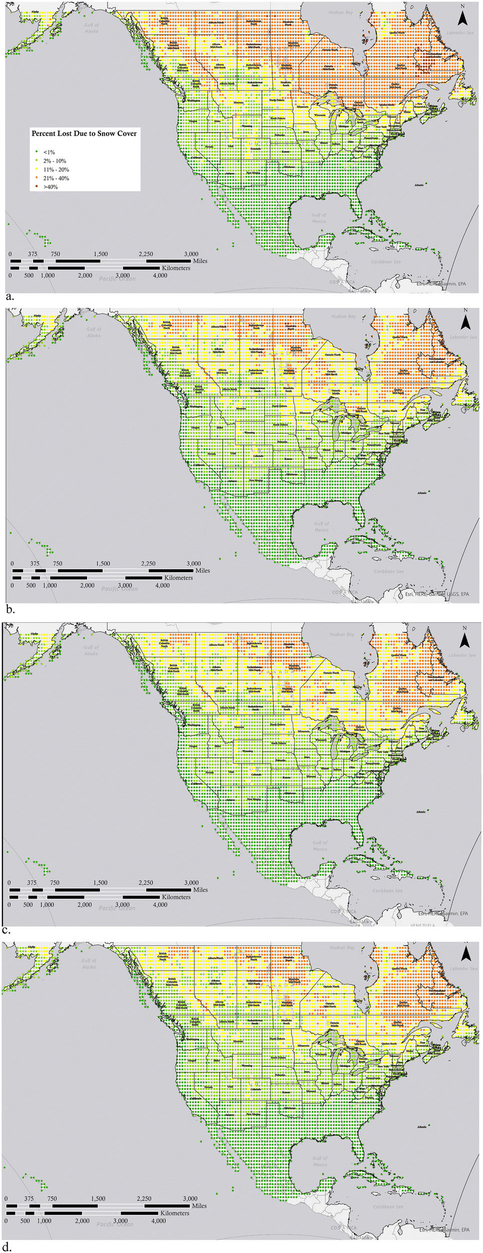 | ||
| Fig. 1 The percent of solar PV losses due to snow based on the sum of hourly losses from snow cover for (a) 2019, and then calculated for the optimistic SSP126 scenario in (b) 2040, (c) 2080 and (d) 2100. | ||
As can be seen by comparing the maps in Fig. 1 and similarly those in Fig. 2, the change between climate prediction years is subtle. This is due to geographical variations and their impact on the climate models. Thus, to clarify this change the percent change in PV potential lost due to snow cover in are shown in Fig. 3 for the optimistic SSP126 scenarios between 2019 and the modeled years of (a) 2040, (b) 2080 and (c) 2100 and the pessimistic SSP585 scenario for (d) 2040, (e) 2080 and (f) 2100.
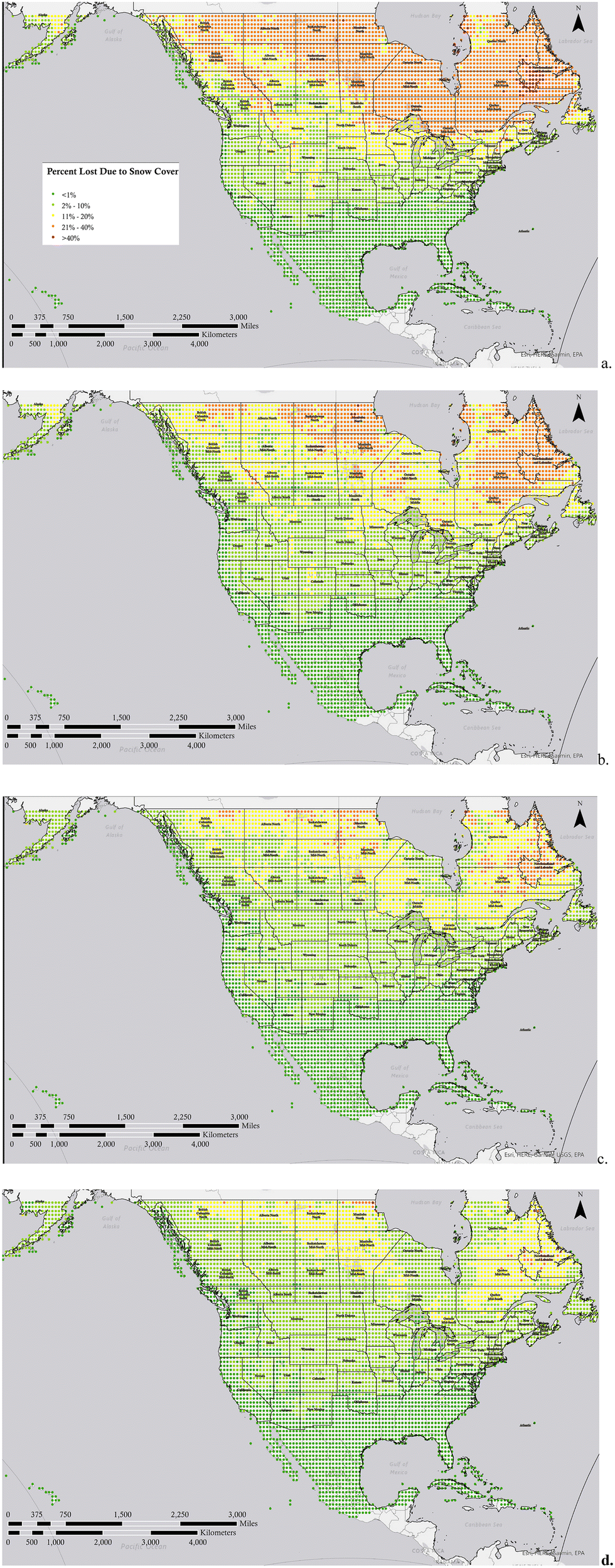 | ||
| Fig. 2 The percent of solar PV losses due to snow based on the sum of hourly losses from snow cover for (a) 2019, and then calculated for the pessimistic SSP585 scenario in (b) 2040, (c) 2080 and (d) 2100. | ||
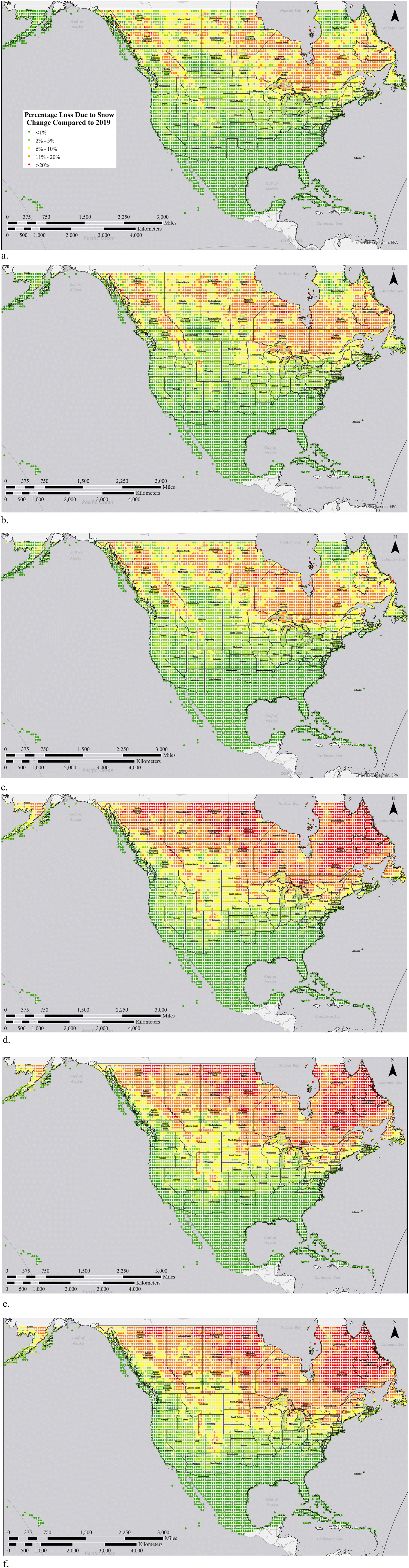 | ||
| Fig. 3 The percent change in PV potential lost due to snow cover for the optimistic SSP126 scenarios between 2019 and the modeled years of (a) 2040, (b) 2080 and (c) 2100 and the pessimistic SSP585 scenario for (d) 2040, (e) 2080 and (f) 2100. | ||
Comparing these changes in percent losses is instructive for determining what regions are most likely to see a substantial change in snow losses. So, for example, comparing Fig. 3a and d the most extreme changes are far larger and move into the U.S. in the pessimistic scenario.
Fig. 4 shows the quantification of the expected snow losses in each state and latitude sliced province for the U.S. and Canada for the 2100 optimistic SSP126 scenarios in Fig. 4a and the pessimistic SSP585 scenario in Fig. 4b. The U.S. states such as Idaho, Pennsylvania, Nebraska, Connecticut, Massachusetts and Utah that have high single digit snow losses in 2019 drop to 5% or less even in the optimistic global warming scenario. Similar behavior is shown for Provinces like Prince Edward Island, Nova Scotia, and British Columbia, the latter loses essentially all snow losses from a 3% base year in 2019.
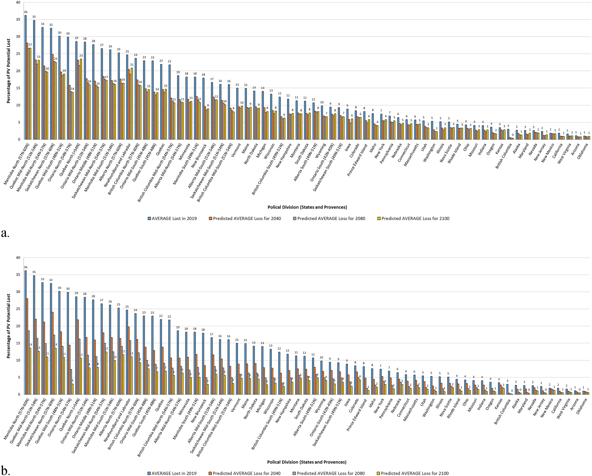 | ||
| Fig. 4 The expected snow losses in each state and latitude sliced province for the U.S. and Canada for (a) the optimistic SSP126 scenarios and (b) the pessimistic SSP585 scenario arranged by highest to lowest percentage loss. | ||
In the pessimistic global warming case the loss reductions are even more striking. So, for example, what are currently very snowy states in the U.S. like Minnesota, Vermont, Maine, North Dakota, and Michigan drop from mid teen annual snow losses to under 5% and in the case of Michigan down to 3%. The changes are even more radical in Canada. As many of the Canadian provinces are so large they were further broken down by latitude. Thus, for example southern Manitoba (59N to 51N) drops from 18% losses to 5%, southern Alberta (49N–51N) drops from 11% losses to 5%, southern Ontario (42N–45N) drops from 9% losses to 3% and even southern Saskatchewan (49N–51N) from 9% losses to only 4%.
There are two issues that need further clarification from a close analysis of the data. First, is that lumping an entire state or even the latitude separations used here for estimating snow losses can lead to errors. For example, in southern Ontario where experiments have shown a range of losses, the 9% for 2019 is taking a geographical weighted average not the population weighted average, so there are fairly far north regions that make the losses appear higher than most PV systems would have in the Province.
Second, as the globe warms under either the optimistic or pessimistic scenarios it is clear that in some regions after the initial massive shift in losses to 2040 in some areas the snow losses actually increase. This is only observed in the optimistic SSP126 scenario. For example, Iowa starts off with an average PV snow loss of 9%, drops under 5% by 2080, but then the losses increase to 6% by 2100. To further analyze this phenomena, the monthly mean temperature changes for 2040 and 2100 in the SSP126 scenario is shown in Fig. 5.
 | ||
| Fig. 5 Difference between 2100 projected monthly mean daily maximum temperatures and 2040 projected monthly mean daily maximum temperatures as a function of month of the year in the SSP126 scenario for (a) January, (b) February, (c) March, (d) April, (e) May, (f) June, (g) July, (h) August, (i) September, (j) October, (k) November, and (l) December. | ||
First, it is clear from Fig. 5 the increase in temperature from 2040 to 2100 is highly non-uniform and changes substantially from month to month. In January the largest changes are mostly confined to the north west, while in February a corridor of less intense change opens up between northern Alaska and the great lakes, then by March the great lakes region is actually colder in 2100 then 2040. Similarly, in November southern Ontario sees an enormous increase in temperature from 2040 to 2100, but there is very little snow normally there. By December, however, there is no change from 2040 to 2100. These complex dynamics coupled with the availability of snow occurring only at freezing or below explain why in some of the regions in the optimistic warming case the snow losses can increase as the earth warms.
This study has several limitations that could be improved in future work. First, it only covers the sensitivity of an optimistic and pessimistic scenarios. There are many other scenarios used by the climate change research community that could be investigated. Secondly, because of the large geographic regions analyzed granular local impacts would have been averaged away so detailed ground truthing is needed from experimental systems. Lastly, the snow loss model used was the Marion model, which does not represent all of the experimental studies available (e.g. the difference between frame and frameless snow sliding ratios) so more detailed models could be used in the future and the results compared to reduce the error associated with a single snow loss percent value. Care must be taken in PV snow related study locations to ensure that they are representative for the regions they are targeting. Despite these limitations the trends in the results of this study are clear and valid even if the percent error is off in a systematic way for a given PV array because of the snow model selected.
Conclusions
The results of this study have shown that in North America as the climate changes and the region warms the PV losses due to snow will be substantially reduced. Even in the most optimistic SSP126 scenario from a climate destabilization perspective, in the next 20 years many currently heavily populated areas in the northern U.S. and southern Canada will decrease to less than the 5% snow loss annual threshold for PV system performance. This amount of loss can still be the pivotal point between solar system profitability. In the more pessimistic SSP585 scenario regions currently known for high volumes of snow become nearly snowless and PV system design needs to adapt. Future work is needed to do more granular simulations of the interplay between the increase in temperature from climate change impacting PV performance including (i) operating temperature (negative), (ii) snow losses (positive), (iii) increased rain-based cleaning (positive) and (iv) albedo decrease (negative). Overall, the trends are clear that climate change is shrinking and in some cases eliminating the snow losses for solar photovoltaic systems from enormous swaths of North America. It is concluded that the reduction in snow losses for a PV systems in the northern latitudes due to climate change should be included in modeling of the life cycle system performance.Methods
All the code for this project is released under a GNU General Public License (GPL) 3.0 and data is available on the Open Science Framework.50Data
This study utilized the irradiance and snow modules within the open source PVLIB library for Python44,45 to model hourly coverage of PV modules by snow and calculate percent of potential energy generation loss. This process requires the following data elements at hourly time steps:• Snowfall
• Air temperature (observed and predicted)
• Plane of Array Irradiance (solar radiation data)
– Surface Tilt
– Surface azimuth
– Solar zenith
– Solar azimuth
– Dni
– Dhi
– Ghi
– Albedo
The year 2019 was selected as a baseline year due to the availability of input datasets. The northern western hemisphere was selected as a study area due to the availability of overlapping data coverage in this area. Sources for these data include the:
• Canadian Meteorological Centre (CMC) Daily Snow Depth Analysis Data, Version 141
• National Renewable Energy Laboratory (NREL) National Solar Radiation Database (NSRDB) 2019 PDS data.42
• WorldClim BCC-CSM2-MR downscaled CMIP6 projections for future climate data using ssp126 and ssp585 scenarios.43
Input data preparation
The CMC Daily Snow depth raster dataset41 was used as a template for this 24 km spacing, and NSRDB Sites that were closest to the center of each pixel in the CMC Daily Snowfall raster dataset. This process was completed in the ESRI ArcGIS Desktop GIS program by first performing a raster-to-feature function, producing a point feature layer from the center of each CMC Daily Snowfall (Band 1) raster pixel. Similarly, the numpy ‘savetxt’ function in Python was used (https://osf.io/c7mv6/) to extract the coordinates of all NSRDB Sites to a csv format file, which was then added to ArcMap and mapped using the ‘place x, y coordinate’ function.
This Snowfall pixel center point layer was then used as the join-to layer in a spatial join function with the NSRDB Sites layer. This process added the index of the NSRDB Site nearest to each Snowfall pixel center point. The result of this join titled ‘selected_sites’ was then exported to an ESRI Shapefile format (https://osf.io/b49sr/) including attributes for the site index, site x coordinate, and site y coordinate.
Additionally, because the snow-loss functions of pvlib.snow use hourly time step data, and to enable more efficient computing, each necessary dataset within the half-hourly NSRDB dataset was sliced at an hourly time step, for each selected site (https://osf.io/6h2pk/), to result in a ‘Short-NSRDB’ (SNSRDB) database (https://osf.io/bwq9e/). All subsequent functions and calculations use this S-NSRDB data for selected sites at hourly timesteps.
The CMC Snow Depth data is provided in a polar projection, centered on the north pole. To align with NSRDB data, this CMC Snow depth data was reprojected to the Web Mercator projection (EPSG:3857) using the warp method within the rasterio library for Python (https://osf.io/nbq5u/).
CMC Snow Depth data are provided as multi-band raster datasets in GeoTiff format. Estimated snow depth for each day are stored within each individual raster band. Daily difference in snow depth were calculated for the full spatial and temporal extent of the CMC Snow Depth data utilizing the rasterio library for Python. The full tiff dataset was loaded into python using the rasterio load function, and each individual raster band was loaded into an array. For each daily band, the snow depth of the previous day was subtracted from the current day, to yield a daily snow depth difference array (https://osf.io/vfzp3/). Each daily snow depth difference array was added as a band to a new output geotiff raster dataset (https://osf.io/a2cyd/).
The rasterstats package in Python (https://pythonhosted.org/rasterstats/) was also utilized to extract raster values at points, using the point_query method [https://pythonhosted.org/rasterstats/manual.html] with previously created ‘selected_sites’ shapefile for input points, and the daily-snow-depth-difference raster bands as raster input (https://osf.io/ar54c/). This resulted in an output array of daily snow depth change values having columns for each site and rows for each day (https://osf.io/fuy8m/).
Because the PVLIB snow loss modules require snowfall at an hourly time step, hourly snowfall rates were estimated by redistributing the calculated daily snowfall at each site equally to each hour of each day (https://osf.io/ncdvu/). This resulted in a dataset of hourly snow depth change values with rows for each site and columns for each hour, which is then transposed when used with other NSRDB input data to match the NSRDB norm of rows for each time-step and columns for each site (https://osf.io/p29a5/). Future snow fall loss projections are detailed in Section 2.4.1.
Loss model execution for observed conditions
In this study the Marion snow loss model with Ryberg improvements was used.9,46,47 The Marion model is a well-known and validated snow loss model that is used in NREL's SAM simulation software. This model calculates the percentage of a PV array covered by snow given: (a) daily snow depth measurements, (b) hourly system tilt, (c) POA irradiance, and (d) temperature values. Backed up with many experimental studies, the Marion model uses snow sliding as the dominant snow removal method and thus does not account for melting, sublimation or wind removal for fix tilted systems. At the start of every day, the model determines if snowfall has occurred and if so it assumes the PV array is completely covered and adds the new snowfall to the previous day. Every hour, the PV remains covered unless the total amount of radiation and ambient temperature are sufficient for accumulated snow to slide off the PV array based on empirical values from Marion. Ryberg improved the temporal resolution and thus checks for snow every hour instead of every day and accounted for sub-hourly calculations. The snow model is the same as the Marion model, except that the sliding coefficient and the delta threshold, are both scaled by the inverse of the number of time steps in an hour, instead of every hour. This results in a more accurate model.46,47 It should be pointed out that there is no completely accepted method for snow loss modeling and that there is substantial variance from all models in a wide array of geographic locations with heavy snow, but the Marion model has been validated in several locations.51 The Marion model has the potential to be highly accurate, but is more vulnerable to uncertainties in snow depth measurement than Townsend model.51 To reduce the error in the Marion model that is built into the open source SAM developed by NREL, the default snow sliding coefficient of 1.97 needs to be tuned. More advanced models are necessary to model every type of PV system (e.g. frame vs frameless modules),52 but the general model works with most standard systems.Output includes an hourly percent coverage by snow and percent DC loss for each time step, at each site and output in HDF5 format (https://osf.io/vh8rx/). Thus, the snow coverage results in an amount of energy that is lost for each hour and scaled to the solar flux that hour that is available. An additional script (https://osf.io/5qeb3/) exports a summary table including the sum of percent loss for all time steps, at each site. This provides a cumulative sum of total potential PV% lost over one year, for each site, output in csv format (https://osf.io/xbmyr/) for use in map and chart visualization.
Preparation of predicted future parameters
The monthly mean daily minimum and maximum temperatures for 2019 were calculated using the resample method in python for time series data. The average of the 2019 monthly mean daily minimum and maximum temperatures was treated as the monthly mean daily temperature for each month in 2019. For each hour in 2019, the hourly temperature departure from the monthly daily mean was calculated to yield an hourly departure from monthly daily mean. This departure from the monthly daily mean was then divided by the monthly daily maximum to yield an hourly deviation from monthly mean daily temperature as a percentage of the daily maximum temperature.
Similarly, for each month in each predicted future year, the average of the predicted monthly mean daily minimum and maximum temperatures was treated as the predicted monthly mean daily temperature for each month in each future year. To calculate a predicted future hourly temperature, the predicted monthly daily mean temperature is added to the product of the 2019 hourly percentage of daily maximum temperature multiplied by the predicted monthly mean daily maximum temperature.
An example of calculating the 2040 hourly temps using observed 2019 hourly temps and projected 2021–2040 monthly mean daily temperature predictions follows: ((2040 modeled monthly mean daily minimum temp + 2040 modeled monthly mean daily maximum temp)/2) + (2019 hourly % of monthly mean daily maximum temperature × 2040 monthly mean daily maximum temperature).
Mapping and summary
Output summary tables of the percentage of potential PV generation loss due to snow coverage at each site (https://osf.io/zuskc/) were added to ArcGIS ArcMap and joined to the ‘selected_sites’ shapefile representing selected site locations. Point locations were symbolized by the percent_loss for each modeled year (2019, 2040, 2080, 2100). It should be pointed out that some sites located along the ocean and Hudson Bay coastlines exhibited 2040 loss projections in excess of 50%. These excessive loss projections are caused by ‘no data’ values in the projected future temperature datasets for sites at these locations, and have been omitted from summaries and map documents.Losses at each site, for each time period and scenario, have been mapped and summarized by political subdivision for the purpose of chart and graph production. Canadian provinces were further subdivided into several sections along multiple lines of Latitude (see Appendix A). Summaries were prepared using the spatial join function in ArcMap to join all site locations within a political division polygon to that polygon, and summarizing them as a mean loss within each polygon. Because some political divisions consisted of more than one polygon, a dissolve function in ArcMap was used to summarize all parts of a division together, again using the mean. This produces a table of mean modeled PV potential loss due to snow for each political division and sub-division, for each time period and scenario (https://osf.io/w289j/).
Conflicts of interest
There are no conflicts to declare.Appendix A
Acknowledgements
This work was supported by the Thompson Endowment.References
- IEA, [cited 2023 Aug 9], Renewable Energy Market Update 2021 – Analysis. Available from: https://www.iea.org/reports/renewable-energy-market-update-2021.
- B. L. Brench, Snow-covering effects on the power output of solar photovoltaic arrays, Massachusetts Inst. of Technology (MIT), Lexington, MA (United States). Lincoln Lab.; 1979 Dec [cited 2023 Aug 8]. Report no. COO-4094-61. Available from: https://www.osti.gov/biblio/5232456.
- R. E. Pawluk, Y. Chen and Y. She, Photovoltaic electricity generation loss due to snow–A literature review on influence factors, estimation, and mitigation, Renewable Sustainable Energy Rev., 2019, 107, 171–182 CrossRef.
- N. Heidari, J. Gwamuri, T. Townsend and J. M. Pearce, Impact of snow and ground interference on photovoltaic electric system performance, IEEE J. Photovolt., 2015, 5(6), 1680–1685 Search PubMed.
- K. S. Hayibo, A. Petsiuk, P. Mayville, L. Brown and J. M. Pearce, Monofacial vs bifacial solar photovoltaic systems in snowy environments, Renewable Energy, 2022, 193, 657–668 CrossRef.
- L. Powers, J. Newmiller and T. Townsend, Measuring and modeling the effect of snow on photovoltaic system performance, in 2010 35th IEEE Photovoltaic Specialists Conference, IEEE, 2010 Jun 20, pp. 000973–000978.
- T. Townsend and L. Powers, Photovoltaics and snow: An update from two winters of measurements in the Sierra, in 2011 37th IEEE Photovoltaic Specialists Conference, IEEE, 2011 Jun 19, pp. 003231–003236.
- J. L. Braid, D. Riley, J. M. Pearce and L. Burnham, Image Analysis Method for Quantifying Snow Losses on PV Systems, In 2020 47th IEEE Photovoltaic Specialists Conference (PVSC), Calgary, AB, Canada: IEEE, 2020, pp. 1510–1516. Available from: https://ieeexplore.ieee.org/document/9300373/.
- B. Marion, R. Schaefer, H. Caine and G. Sanchez, Measured and modeled photovoltaic system energy losses from snow for Colorado and Wisconsin locations, Sol. Energy, 2013, 97, 112–121 CrossRef.
- T. Sugiura, T. Yamada, H. Nakamura, M. Umeya, K. Sakuta and K. Kurokawa, Measurements, analyses and evaluation of residential PV systems by Japanese monitoring program, Sol. Energy Mater. Sol. Cells, 2003, 75(3–4), 767–779 CrossRef CAS.
- T. Matthews, Solar photovoltaic reference array report, Northern Alberta Institute of Technology, 2016.
- M. Taylor, Statistical Relationship Between Photovoltaic Generation and Electric Utility Demand in Minnesota (1996–2002), in Proceedings of the Solar Conference, American Solar Energy Society, American Institute of Architects, 2003, pp. 213–218.
- R. W. Andrews, A. Pollard and J. M. Pearce, The effects of snowfall on solar photovoltaic performance, Sol. Energy, 2013, 92, 84–97 CrossRef.
- R. W. Andrews and J. M. Pearce, Prediction of energy effects on photovoltaic systems due to snowfall events, in 2012 38th IEEE Photovoltaic Specialists Conference, Austin, TX, USA, IEEE, 2012, pp. 003386–003391. Available from: http://ieeexplore.ieee.org/document/6318297/.
- M. M. Ross, Snow and ice accumulation on photovoltaic arrays: An assessment of the TN conseil passive melting technology, report# EDRL 95-68 (TR), energy diversification research laboratory, CANMET, Natural Resources Canada, Varennes, 1995 Sep.
- R. W. Andrews and J. M. Pearce, The effect of spectral albedo on amorphous silicon and crystalline silicon solar photovoltaic device performance, Sol. Energy, 2013, 91, 233–241 CrossRef CAS.
- E. Molin, B. Stridh, A. Molin and E. Wäckelgård, Experimental yield study of bifacial PV modules in nordic conditions, IEEE J. Photovolt., 2018, 8(6), 1457–1463 Search PubMed.
- N. Riedel-Lyngskær, M. Ribaconka, M. Pó, A. Thorseth, S. Thorsteinsson, C. Dam-Hansen and M. L. Jakobsen, The effect of spectral albedo in bifacial photovoltaic performance, Sol. Energy, 2022, 231, 921–935 CrossRef.
- L. Burnham, D. Riley, B. Walker and J. M. Pearce, Performance of Bifacial Photovoltaic Modules on a Dual-Axis Tracker in a High-Latitude, High-Albedo Environment. In, 2019 IEEE 46th Photovoltaic Specialists Conference (PVSC), Chicago, IL, USA, IEEE; 2019 [cited 2023 Aug 9], pp. 1320–1327. Available from: https://ieeexplore.ieee.org/document/8980964/.
- B. P. Jelle, T. Gao, S. A. Mofid, T. Kolås, P. M. Stenstad and S. Ng, Avoiding snow and ice formation on exterior solar cell surfaces–a review of research pathways and opportunities, Procedia Eng., 2016, 145, 699–706 CrossRef.
- R. W. Andrews, A. Pollard and J. M. Pearce, A new method to determine the effects of hydrodynamic surface coatings on the snow shedding effectiveness of solar photovoltaic modules, Sol. Energy Mater. Sol. Cells, 2013, 113, 71–78 CrossRef CAS.
- A. Kahl, J. Dujardin and M. Lehning, The bright side of PV production in snow-covered mountains, Proc. Natl. Acad. Sci. U. S. A., 2019, 116(4), 1162–1167 CrossRef CAS PubMed.
- A. Rahmatmand, S. J. Harrison and P. H. Oosthuizen, An experimental investigation of snow removal from photovoltaic solar panels by electrical heating, Sol. Energy, 2018, 171, 811–826 CrossRef.
- A. Weiss and H. Weiss, Photovoltaic cell electrical heating system for removing snow on panel including verification, in 2016 IEEE International Conference on Renewable Energy Research and Applications (ICRERA), IEEE, 2016 Nov 20, pp. 995–1000.
- S. Hosseini, S. Taheri, M. Farzaneh and H. Taheri, Modeling of snow-covered photovoltaic modules, IEEE Trans. Ind. Electron., 2018, 65(10), 7975–7983 Search PubMed.
- B. Hashemi, S. Taheri and A. M. Cretu, Systematic analysis and computational intelligence based modeling of photovoltaic power generation in snow conditions, IEEE J. Photovolt., 2021, 12(1), 406–420 Search PubMed.
- M. van Noord, T. Landelius and S. Andersson, Snow-induced PV loss modeling using production-data inferred PV system models, Energies, 2021, 14(6), 1574 CrossRef.
- G. Wirth, M. Schroedter-Homscheidt, M. Zehner and G. Becker, Satellite-based snow identification and its impact on monitoring photovoltaic systems, Sol. Energy, 2010, 84(2), 215–226 CrossRef.
- S. Pelland, G. Galanis and G. Kallos, Solar and photovoltaic forecasting through post-processing of the Global Environmental Multiscale numerical weather prediction model, Prog. Photovoltaics Res. Appl., 2013, 21(3), 284–296 CrossRef.
- E. Lorenz, D. Heinemann and C. Kurz, Local and regional photovoltaic power prediction for large scale grid integration: Assessment of a new algorithm for snow detection, Prog. Photovoltaics Res. Appl., 2012, 20(6), 760–769 CrossRef.
- M. B. Øgaard, B. L. Aarseth, Å. F. Skomedal, H. N. Riise, S. Sartori and J. H. Selj, Identifying snow in photovoltaic monitoring data for improved snow loss modeling and snow detection, Sol. Energy, 2021, 223, 238–247 CrossRef.
- J. Cook, N. Oreskes, P. T. Doran, W. R. Anderegg, B. Verheggen, E. W. Maibach, J. S. Carlton, S. Lewandowsky, A. G. Skuce, S. A. Green and D. Nuccitelli, Consensus on consensus: a synthesis of consensus estimates on human-caused global warming, Environ. Res. Lett., 2016, 11(4), 048002 CrossRef.
- W. R. Anderegg, J. W. Prall, J. Harold and S. H. Schneider, Expert credibility in climate change, Proc. Natl. Acad. Sci. U. S. A., 2010, 107(27), 12107–12109 CrossRef CAS PubMed.
- N. Oreskes, The scientific consensus on climate change: How do we know we’re not wrong?, Springer International Publishing, 2018 Search PubMed.
- Climate Change 2013: The Physical Science Basis: Working Group I Contribution to the Fifth Assessment Report of the Intergovernmental Panel on Climate Change, ed. T. Stocker, Cambridge University Press, 2014.
- M. Allen, O. P. Dube, W. Solecki, F. Aragón-Durand, W. Cramer, S. Humphreys and M. Kainuma, Special Report: Global Warming of 1.5 C. Intergovernmental Panel on Climate Change (IPCC), 2018 Oct.
- R. Alley, T. Bernsten, N. Bindoff, Z. Chen, A. Chidthaisong, P. Fredlingstein, J. Gregory, et al., AR4 Climate Change 2007: The Physical Science Basis: Summary for Policy Makers, Geneva: IPPC Secretariat: Intergovernmental Panel on Climate Change.
- F. Creutzig, P. Agoston, J. C. Goldschmidt, G. Luderer, G. Nemet and R. C. Pietzcker, The underestimated potential of solar energy to mitigate climate change, Nat. Energy, 2017, 2(9), 1–9 Search PubMed.
- M. Jaxa-Rozen and E. Trutnevyte, Sources of uncertainty in long-term global scenarios of solar photovoltaic technology, Nat. Clim. Change, 2021, 11(3), 266–273 CrossRef.
- E. R. Siirila-Woodburn, A. M. Rhoades, B. J. Hatchett, L. S. Huning, J. Szinai, C. Tague, P. S. Nico, D. R. Feldman, A. D. Jones, W. D. Collins and L. Kaatz, A low-to-no snow future and its impacts on water resources in the western United States, Nat. Rev. Earth Environ., 2021, 2(11), 800–819 CrossRef.
- National Snow and Ice Data Center. 2021 [cited 2023 Aug 9], Canadian Meteorological Centre (CMC) Daily Snow Depth Analysis Data, Version 1. Available from: https://nsidc.org/data/nsidc-0447/versions/1.
- NREL National Solar Radiation Database – Registry of Open Data on AWS. [cited 2023 Aug 9], Available from: https://registry.opendata.aws/nrel-pds-nsrdb/.
- Future climate data—WorldClim 1 documentation, [cited 2023 Aug 9], Available from: https://www.worldclim.org/data/cmip6/cmip6climate.html.
- pvlib python documentation, [cited 2023 Aug 9], Available. https://pvlib-python.readthedocs.io/en/stable/index.html.
- W. F. Holmgren, C. W. Hansen and M. A. Mikofski, pvlib python: A python package for modeling solar energy systems, J. Open Source Softw., 2018, 3(29), 884 CrossRef.
- D. Ryberg and J. Freeman, Integration, validation, and application of a PV snow coverage model in SAM, National Renewable Energy Laboratory, Golden, CO, USA, 2015 Sep 1.
- J. M. Freeman and D. S. Ryberg, Integration, Validation, and Application of a PV Snow Coverage Model in SAM (No. NREL/TP-6A20-68705), National Renewable Energy Lab. (NREL), Golden, CO (United States), 2017.
- L. Bosman and S. Darling, Difficulties and recommendations for more accurately predicting the performance of solar energy systems during the snow season, in 2016 IEEE International Conference on Renewable Energy Research and Applications (ICRERA), IEEE, 2016, pp. 567–571.
- S. Pisklak, Commercial implementation of a snow impact model for PV performance prediction, in 2016 IEEE 43rd Photovoltaic Specialists Conference (PVSC), IEEE, 2016 Jun 5, pp. 1002–1006.
- Future snow losses for PV systems on the Open Science Framework, [cited 2023 Aug 9], Available from: https://osf.io/ndq8e/.
- C. Baldus-Jeursen, A. L. Petsiuk, S. A. Rheault, S. Pelland, A. Côté and Y. Poissant, et al., Snow Losses for Photovoltaic Systems: Validating the Marion and Townsend Models, IEEE J. Photovolt., 2023, 13(4), 610–620 Search PubMed.
- D. Riley, L. Burnham, B. Walker and J. M. Pearce, Differences in snow shedding in photovoltaic systems with framed and frameless modules, in 2019 IEEE 46th Photovoltaic Specialists Conference (PVSC), IEEE, 2019 Jun 16, pp. 0558–0561.
| This journal is © The Royal Society of Chemistry 2023 |