
Soft, flexible conductivity sensors for ocean salinity monitoring†
Shao-Hao
Lu
 a,
Yi
Li
a and
Xueju
Wang
*ab
a,
Yi
Li
a and
Xueju
Wang
*ab
aDepartment of Materials Science and Engineering, University of Connecticut, Storrs, CT 06269, USA. E-mail: xueju.wang@uconn.edu
bInstitute of Materials Science, University of Connecticut, Storrs, CT 06269, USA
First published on 8th June 2023
Abstract
Flexible electrochemical sensors that measure the concentrations of specific analytes (e.g., ions, molecules, and microorganisms) provide valuable information for medical diagnosis, personal health care, and environmental monitoring. However, the conductive electrodes of such sensors need to be exposed to the surrounding environments like chloride-containing aqueous solutions during their operation, where chloride ions (Cl−) can potentially cause corrosion and dissolution of the sensors, negatively impacting their performance and durability. In this work, we develop soft, flexible conductivity sensors made of gold (Au) electrodes and systematically study their electrochemical behaviors in sodium chloride (NaCl) solutions to prevent chloride-induced corrosion and enhance their sensitivity for marine environmental monitoring. The causes of gold chlorination reactions and polarization effects are identified and effectively prevented by analyzing the effects of direct current (DC) and alternating current (AC) voltages, AC frequencies, and exposed sensing areas of the conductivity (salinity) sensors. Accordingly, a performance diagram is constructed to provide guidance for the selection of operation parameters for the salinity sensor. We also convert the varying impedance values of salinity sensors at different salinity levels into output voltage signals using a voltage divider circuit with an AC voltage (0.6 V) source. The results offer an assessment of the accuracy and response time of the salinity sensors, as well as their potential for integration with data transmission components for real-time ocean monitoring. This study has important implications for the development of soft, flexible, Au-based electrochemical sensors that can operate efficiently in diverse biological fluids and marine environments.
 Xueju Wang | Dr Xueju “Sophie” Wang is currently an Assistant Professor in Materials Science and Engineering and affiliated with Biomedical Engineering and the Institute of Materials Science at the University of Connecticut. She obtained her PhD degree in Mechanical Engineering at the Georgia Institute of Technology in 2016 and was a postdoctoral scholar at Northwestern University from 2016 to 2018. Her research interests lie in the intersection of active materials, mechanics, and functional structures for applications ranging from soft robotics to flexible electronics. She is the recipient of the NSF CAREER Award, NIH Trailblazer Award, EML Young Investigator Award, ACS PMSE Young Investigator Award, and ASME ORR Early Career Award. |
1. Introduction
Flexible electronics is an emerging field that holds the potential to revolutionize a wide range of technologies, including wearable devices,1,2 medical diagnosis,3–6 and consumer electronics.7 Wearable and implantable electrochemical sensors are flexible electronic devices designed to measure the concentrations of specific analytes (e.g., ions, molecules, and microorganisms) in the environment.8–11 Their sensing mechanism is based on the principles of electrochemistry, where the interaction (or reaction) between the sensing surface and the chemical/biochemical substances is quantified by applying electrical potential/current to electrodes and detecting corresponding electrical signals. Thus, a common feature of electrochemical sensors is that their sensing electrodes are exposed to the surrounding environments,11–13 like the frequently used chloride-containing aqueous solutions, during operation. For example, biosensors are tested in phosphate-buffered saline (PBS) solutions8,11,14–20 or biological fluids, such as sweat,10,20–23 tears,5,18 saliva,24,25 and interstitial fluids.9,26 Additionally, electrochemical sensors for environmental monitoring and analysis are immersed in seawater,27–30 tap water,31 and soil specimens.32 Among various conductive materials for electrochemical sensors, including carbon-based materials, metal nanomaterials, and conductive polymers, noble metals such as Au, silver (Ag), and platinum (Pt) are versatile electrode materials due to their high electrical conductivity and superior chemical stability.33 However, the exposed sensing area of the metallic electrodes for electrochemical sensors is in direct contact with the chloride ions (Cl−), which can potentially cause the dissolution of the sensors due to chlorination reactions.34,35 Such reactions may negatively impact the performance and durability of the sensor, and, therefore, addressing this issue is critical for the reliability of the sensor measurements.Take the salinity sensor as an example, typical commercial salinity sensors include refractometers and stainless-steel-based conductivity meters that measure the refractive index and electrical conductivity of solutions, respectively, to determine their salinity levels. However, the rigid components in these devices, such as glass lenses in refractometers and stainless-steel electrodes in conductivity meters make them bulky and restrict their versatility in applications that require device flexibility. To overcome these limitations, researchers have developed salinity sensors based on flexible optical fibers that can be integrated with smartphones for more accurate and adaptable data analysis than refractometers.36,37 In addition, stainless-steel thin films that are conformal and could potentially improve the flexibility of stainless-steel electrodes in conductivity meters are reported, in which, however, the stainless-steel thin film is primarily deposited onto rigid metallic substrates (hundreds of micrometers thick) and still limits their flexibility.38 Recently, a flexible conductivity cell with gold thin-film (Au, 100 nm) electrodes for salinity measurements has been reported with improved flexibility.29 Nonetheless, the study showed that the Au electrodes suffered damage when performing measurements in a NaCl solution with an alternating current (AC) of 1 mA.29 In addition, our recent work demonstrated that salinity sensors made of Au electrodes can function under large hydrostatic pressure of up to 15 MPa, but experience damage when being operated at a constant current of 1 μA.39 To address chlorination-induced corrosion problems in salinity sensors, some researchers explored the use of carbon-based electrodes, such as laser-induced graphene (LIG) on a polyimide substrate, as an alternative material for flexible salinity sensors.29,40 Nevertheless, bending the LIG conductivity sensor causes the stretching of its porous graphene structure, which increases the sensing area exposed to the saline solution and leads to a transconductance increase of over 50% at the same salinity level.29
In this work, we perform a systematic study on the electrochemical behavior of Au electrodes in sodium chloride (NaCl) solutions to reveal the cause of the gold chlorination reactions and enhance the performance of soft salinity sensors for ocean environmental monitoring. Au thin films are chosen as the model material for this study because of their biocompatibility, chemical inertness, and long-term stability. First, direct current (DC) signals with various potentials are applied to investigate the interaction between the Au electrodes and Cl−, and a critical potential of ≤0.8 V is identified to prevent chlorination reactions. Next, various testing parameters, including AC frequencies, AC voltages, and the exposed sensing area of the salinity sensors, are systematically and thoroughly analyzed to optimize the performance of the sensor, leading to a performance diagram that can provide important guidance for the operation of the salinity sensor. Finally, to achieve real-time salinity measurements, we utilize an AC voltage source (square wave, 0.6 V, 1 kHz) and a voltage divider circuit to convert the varying impedance values of salinity sensors at different salinity levels into output voltages. The accuracy and response time are evaluated by recording time-dependent output voltages as the salinity levels vary, which can assess the viability of integrating the developed soft salinity sensor into fully functional electronic systems. Compared with existing salinity sensors, our developed soft, flexible salinity sensors offer the advantages of (1) thin geometry and potential for miniaturization, (2) high flexibility, (3) real-time monitoring, (4) high pressure tolerance and high energy efficiency, and (5) potential for integration with many platforms including animal tags, divers, and soft robotics.
2. Results and discussion
Design concept of soft, flexible salinity sensors for ocean monitoring
Soft, flexible ocean sensors can enable conformal integration onto various platforms, such as marine creatures and soft robots, and realize real-time marine environmental monitoring. As shown in Fig. 1A, our flexible salinity sensor comprises two separated Au electrodes that are fabricated by depositing Au thin films (thickness of 100 nm) onto a soft substrate of bi-layer parylene C (5 μm) and polyimide (PI, 7.6 μm) using magnetron sputtering, and patterning of the Au film into desired geometries (dimensions of 4 mm × 4 mm) via photolithography. A chromium thin film (Cr, 10 nm) serves as an adhesion layer between Au and parylene C. Encapsulating the sensor with a 5 μm-thick layer of parylene C from the top followed by reactive ion etching defines exposed areas on the Au electrodes and enables the protection of the parylene C-covered regions from the potentially corrosive environment. As shown in the exploded view of the salinity sensor (Fig. 1A), there are two pairs of exposed areas for the two Au electrodes: the inner pair of exposed areas in contact with the saline water is used for ion sensing and conductivity measurement, and the outer pair of exposed areas serves as contact pads where conductive wires are soldered for power supply and data acquisition. The optical image in Fig. 1 shows that the fabricated salinity sensor can be laminated onto a soft PDMS substrate, and can be easily held and bent with two fingers, demonstrating its flexibility, miniaturized size, and ease of integration with future ocean monitoring devices. To further evaluate the flexibility of the salinity sensor, we performed additional bending and twisting tests of the sensor. More specifically, for the bending test, we laminated the salinity sensor onto 3D printed molds (material: digital ABS) with bending angles of 0°, 10°, 20°, 30°, 40°, and 50° (insets in Fig. 1B) and submerged the sensor in 30 PSU NaCl solution for testing. Fig. 1B shows the electrical response (relative impedance change of the salinity sensor, recorded by an LCR meter (IM3533, Hioki)) as a function of the bending angle from 0° to 50°. We can see that the impedance of the sensor has negligible changes under varying bending angles. For the twisting test, the salinity sensor was first laminated onto a soft PDMS substrate, which was then manually twisted from an angle of 0° to 90°. Fig. 1C shows the real-time relative impedance change of the salinity sensor as the twisting angle varies from 0° to 90° within 60 seconds, along with the optical images of untwisted and twisted salinity sensors. The impedance of the salinity sensor remains unchanged at a relatively small twisting angle of 0°–30° and experiences a slight increase (up to 1.2%) as the twisting angle increases to 90°. Overall, the bending and twisting tests demonstrate the high flexibility of the salinity sensor, which can be integrated with many platforms.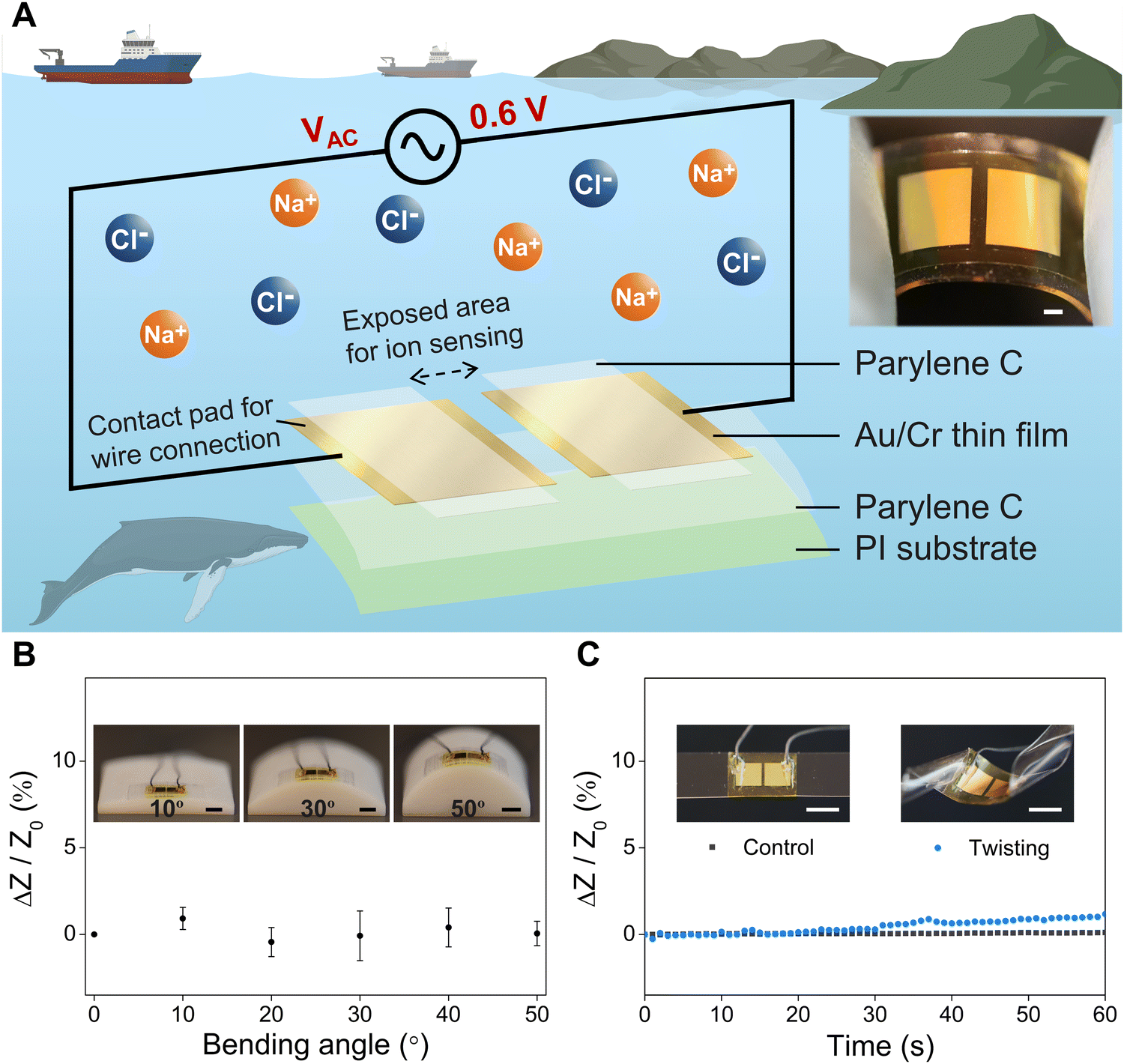 | ||
| Fig. 1 (A) Schematic illustration of the layout and working principle of soft salinity sensors, as well as an optical image of a flexible salinity sensor laminated onto a soft PDMS substrate. Created with BioRender.com. Scale bar in the inset image: 1 mm. (B) Bending test of the salinity sensor showing the relative impedance change of the sensor as a function of bending angles from 0° to 50°. Scale bars: 5 mm. (C) Twisting test of the salinity sensor showing the real-time relative impedance change of the sensor under a twisting angle from 0° to 90° in 60 seconds. Scale bars: 5 mm. | ||
For the practical application of salinity sensors in the ocean environment, it is crucial to ensure that the Au electrodes function effectively for a reasonable period of time in seawater which contains approximately 35 g NaCl/L (35 PSU) on average. Although Au is a widely used electrode material due to its outstanding chemical stability and oxidation resistance, the presence of halide ions (Cl− or Br−) in seawater and the applied operation voltage on the electrodes can trigger the electrolysis reaction of Au and accelerate the dissolution of Au electrodes. To prevent such reaction, we employ various electrochemical analysis techniques in this study to investigate the effects of the direct current (DC) voltage, alternating current (AC) frequency and AC voltage on the performance of salinity sensors (will be discussed in the following section). An AC voltage with an amplitude of 0.6 V is identified as the optimal test potential to prevent damage to the Au electrode and overcome the limitations of DC voltage by oscillating the ions between the electrodes.
The effect of applied DC voltages on the performance of salinity sensors
To determine the optimal voltage for salinity measurement in the ocean environment, the response current of the salinity sensor is measured under voltages of 0–1.5 V using linear sweep voltammetry (LSV) at salinity levels of 30–40 PSU. This electroanalytical method involves sweeping the potential of a working electrode over a defined potential range while measuring the response current (direct current, DC) flowing through the electrodes, which is utilized to identify the reduction-oxidation (redox) electrochemical reactions and to quantify the electroactive species in a solution. Fig. 2A shows the LSV curves of salinity sensors tested with an applied potential range of 0–1.5 V. At the beginning, the curves under different NaCl concentrations increase very slowly and highly overlap with each other. However, all LSV curves at different salinity levels start rising at 0.8 V (zoom-in curves in Fig. 2A), indicating that a redox reaction occurs at this potential. Based on the potential-pH diagram (Pourbaix diagram) of the gold-chloride-water system, which investigates the electrochemical behavior of Au in NaCl solution and plots the theoretical potential of reduction reactions, Au reacts with chloride ions through the following reactions and forms AuCl2− and AuCl4− anions when the potential exceeds 0.8 V.35,41Au + 2Cl− → AuCl2− + e− E0 (V) = 1.15 − 0.1183![[thin space (1/6-em)]](https://www.rsc.org/images/entities/char_2009.gif) log(Cl−) + 0.0592log(AuCl2−) log(Cl−) + 0.0592log(AuCl2−) | (1) |
| Au + 4Cl− → AuCl4− + 3e− E0 (V) = 1.002 − 0.079log(Cl−) + 0.0197log(AuCl4−) | (2) |
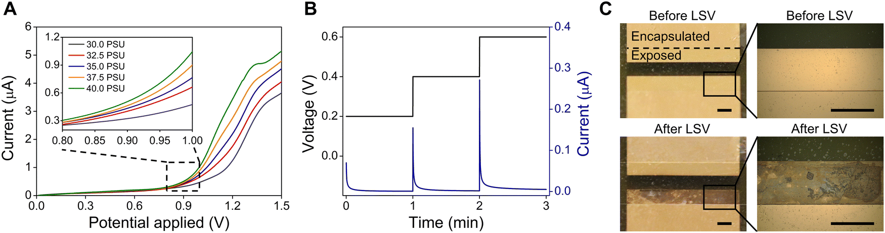 | ||
| Fig. 2 (A) Linear sweep voltammetry (LSV) curves of salinity sensors measured in NaCl solutions at salinity levels of 30–40 PSU. (B) Applied voltage-time waveform and response current-time profile measured by chronoamperometry at a salinity of 30 PSU. (C) Optical images of the salinity sensor before and after LSV measurements scanned in the potential range of 0–1.5 V. Scale bars: 500 μm. | ||
These chlorination processes also produce electrons and drive an electric current that corresponds to the rise of LSV current response at 0.8–0.9 V. This clearly explains the reason why the previous research applied a constant AC current of 1 mA on their four-electrode conductivity cell and observed severe damage to the outer pair of Au electrodes.29 Under their operating conditions, the high resistance of the conductivity sensor (R = 1/G > 800 Ω) can lead to the voltage between the two electrodes above 0.8 V (V = 800 Ω × 1 mA), which exceeds the chlorinating potential and cause Au dissolution. Therefore, the optimal condition for salinity measurement is the constant voltage mode below 0.8 V, where the chlorination reactions can be avoided to prevent Au electrodes from corrosion and dissolution in NaCl solution. In addition, response currents under different NaCl concentrations become differentiable at an applied potential of above 1.2 V, with the maximum current variations observed at 1.35 V (2.98 μA at 30 PSU and 4.70 μA at 40 PSU), which is consistent with the standard reduction potentials of chlorine/chloride ions (E0 = 1.36 V).
Chronoamperometry, a time-dependent current (DC) measurement at steps of constant potential, is then performed to study the kinetics of charge transport at applied voltages below 0.8 V. Here, three steps of constant potential (0.2 V, 0.4 V, and 0.6 V) are applied to the salinity sensor in a 30 PSU NaCl solution and the response current is recorded for 1 min at each step. As shown in the applied voltage-time waveform (Fig. 2B left y-axis) and response current-time profile (Fig. 2B right y-axis), the initial currents for each step are 0.07 μA, 0.15 μA and 0.27 μA, respectively. However, the current drops rapidly and down to below 0.005 μA within 1 minute regardless of the applied voltage value. The sharp decline in current is due to the migration of Na+ and Cl− ions, which gradually accumulate near the electrode surfaces, eventually blocking the current flow between the two electrodes. This phenomenon, which is known as the polarization effect, may negatively affect the accuracy of conductivity measurements.42,43 According to Ohm's law (R = V/I), the calculated resistance of the salinity sensor would soar from 2.2 MΩ to 122.5 MΩ within 1 minute of testing at the constant voltage of 0.6 V. Consequently, despite solving the issue of electrode damage, applying a DC voltage below 0.8 V is not suitable for salinity measurements because it restricts the mobility of ions and causes significant errors in resistance measurements.
The optical microscope images of the salinity sensor captured before and after LSV measurements confirm that the Au electrodes undergo the electrolysis reactions at a sweeping voltage range of 0–1.5 V. As shown in Fig. 2C, one side of the Au electrode is severely corroded and dissolved after test, indicating the chlorination processes occur at the anode terminal and causes the anodic Au dissolution.
The effect of AC frequency on the performance of salinity sensors
To diminish the polarization effect at low DC voltage (<0.8 V), alternating current (AC) is utilized to keep the charged ions oscillating between electrodes. Electrochemical impedance spectroscopy (EIS) is used to evaluate the changes in the impedance (Z), which quantifies the opposition to AC flowing through the circuit, of salinity sensors to determine salinity levels. EIS measures impedance as a complex number with magnitude (|Z|) and phase angle (Φ) by applying low-amplitude AC voltages over a range of frequencies. Purely resistive impedance (ZR = R) is independent of frequency and has a phase angle of 0°, while purely capacitive impedance (ZC = 1/jωC, ω = 2πf) varies with frequency and its phase angle is −90°.To study the effect of AC frequency on the performance of salinity sensors, the measured impedance magnitude and phase angle are plotted as a function of frequency in Fig. 3A and B, respectively. The impedance of the salinity sensor decreases from approximately 20 kΩ to 100 Ω when the AC frequency increases from 1 kHz to 500 kHz. Most importantly, the impedance curves show a good correlation between impedance values and salinity levels (the lower the salinity, the higher the impedance) at each constant frequency, as shown in the zoom-in view of impedance curves at the frequency of 1 kHz, 10 kHz, and 100 kHz (Fig. 3I–III). The relative impedance change (ΔZ/Z0, %), with Z0 being the impedance at 30 PSU, is also plotted as a function of salinity levels to compare the sensitivity of the salinity sensor at different frequencies.
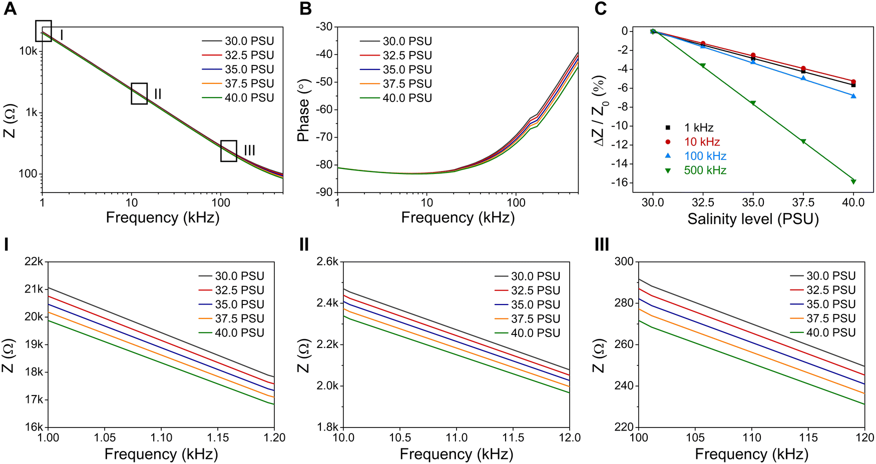 | ||
| Fig. 3 Electrochemical impedance spectroscopy (EIS) curves of salinity sensors with an exposed sensing area of 500 μm tested in NaCl solution at salinity levels of 30–40 PSU. (A) Impedance as a function of frequency in the range of 1–500 kHz. Zoom-in EIS curves at frequencies of (I) 1–1.2 kHz, (II) 10–12 kHz, and (III) 100–120 kHz. (B) Phase angle as a function of frequency in the range of 1–500 kHz. (C) Relative impedance change (ΔZ/Z0, %) as a function of salinity levels at different applied frequencies. | ||
Fig. 3C shows that the AC frequency has a noticeable effect on the performance of the salinity sensor. Overall, the sensitivity (defined as the absolute value of relative impedance change (|ΔZ/Z0|) of the salinity sensor is improved as the AC frequency increases from 1 kHz to 500 kHz. At the frequency of 1 kHz, |ΔZ/Z0| is approximately 5.5% under a salinity change from 30 PSU to 40 PSU. |ΔZ/Z0| increases to 6.9% and 15.8% at 100 kHz and 500 kHz, respectively. Moreover, there is a strong negative correlation between relative impedance changes and phase angles (Fig. S1, ESI†). The minimum relative impedance change at 10 kHz corresponds to its maximum phase angle (−83.2°), and the sharply increased relative impedance change at 500 kHz is correlated to its lowest phase angle (−44.4°). According to Fig. 3A and B, the magnitude of the impedance varies with frequency, and the phase angles are negative, revealing that the salinity sensor tested in NaCl solution contains both resistive and capacitive properties. The capacitive behavior of the salinity sensor in the EIS measurements is associated with the double-layer capacitance that arises from two layers of opposing charged ions at the surface of the electrode. Specifically, the polarization effect is not fully eliminated even under the AC conductivity measurement. Various approaches, such as increasing the electrode surface area, applying an appropriate AC frequency, and using a four-electrode cell, have been reported to weaken the negative impact of double-layer capacitance.42,43 Please note that these approaches are not the focus of this study and will be studied elsewhere.
The effect of AC voltage and exposed sensing areas on the performance of salinity sensors
Impedance measurements using the low-amplitude AC signal (0.01 V) in Fig. 3C have demonstrated the strong linearity between relative impedance changes and salinity levels. In this section, various applied AC voltages and exposed sensing areas are studied to accelerate the ionic transport, reduce the current density, and, therefore, decrease the influence of double-layer capacitance on the performance of the salinity sensor. According to the impedance values measured at AC voltages of 0.01 V, 0.4 V, 0.6 V and 1.0 V (Fig. 4A), a higher applied AC voltage leads to a lower impedance of salinity sensors due to the increased ionic mobility and conductivity. Fig. 4B shows the linear relationship between relative impedance changes and salinity levels under applied AC voltages of 0.01 V–1.0 V. We can see that when being tested under salinity levels of 30 PSU-40 PSU, |ΔZ/Z0| of the salinity sensor increases from 6.8% to 52.3% as the applied AC voltage rises from 0.01 V to 1.0 V, which is attributed to its decreased phase shift angle and reduced polarization (Fig. S2, ESI†). Such results indicate that a larger applied AC voltage could enhance the sensitivity of the salinity sensor. However, as shown in the optical images of salinity sensors before and after salinity measurements (Fig. 4C), the Au electrodes are damaged under 1.0 V VAC as the chlorination processes are activated at voltages above 0.8 V, which is consistent with the study on the effect of DC voltage on salinity sensors earlier. In addition, the AC signal periodically reverses its direction, causing anodic reactions at both terminals and corroding both sides of the Au electrode. Conversely, no degradation of Au electrodes is observed when the salinity sensor is tested at 0.6 V VAC. Thus, as long as the voltage is lower than the redox potential of the gold chlorination reaction (0.8 V), increasing the applied voltage is an effective approach to increase the sensitivity of the salinity measurement.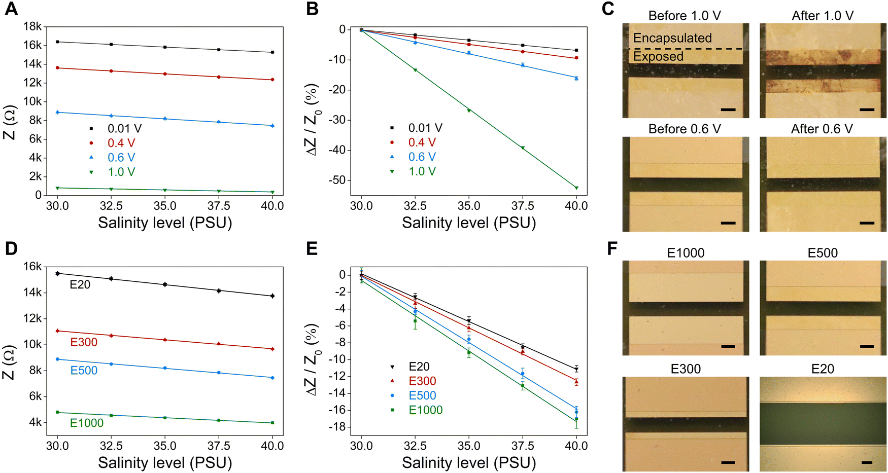 | ||
| Fig. 4 Calibration curves of (A) impedance and (B) relative impedance change (ΔZ/Z0, %) of salinity sensors as a function of salinity levels under VAC of 0.01 V–1.0 V (all sensors have the same exposed sensing area of 500 μm and are tested at a constant frequency of 1 kHz). (C) Optical images of salinity sensors before and after salinity measurements at applied AC voltage of 1.0 V and 0.6 V, respectively. Scale bars: 500 μm. Calibration curves of (D) impedance and (E) relative impedance change (ΔZ/Z0, %) of salinity sensors with various exposed sensing areas as a function of salinity levels (all sensors are tested at a constant frequency of 1 kHz and constant applied VAC of 0.6 V). (F) Optical images of salinity sensors with various exposed sensing areas after salinity measurements. Scale bars: 100 μm for the microscopic image of E20; 500 μm for the rest of the images. | ||
We further study the effect of exposed electrode areas on the performance of the salinity sensor using 0.6 V (AC) to avoid Au dissolution. As described earlier, the 4 mm × 4 mm electrodes are encapsulated by a parylene C layer, and the exposed sensing areas are defined by patterning the parylene C layer via a reaction ion etching (RIE) process. The exposed widths of the electrode sensing areas are 20 μm, 300 μm, 500 μm and 1000 μm, which are denoted as E20, E300, E500 and E1000, respectively. For example, the E20 salinity sensor has a pair of 20 μm × 4 mm exposed regions in contact with the saline solution. Fig. 4D and E show that a larger exposed area results in lower impedance values under the same salinity level and higher relative impedance changes |ΔZ/Z0| over 30–40 PSU. In addition, increasing the exposed area can improve the sensitivity of the salinity sensor, as the resulting lower current densities (Table S1, ESI†) are accompanied with a reduced polarization effect. The optical images of salinity sensors in Fig. 4F show various exposed areas after salinity measurements, confirming that the salinity sensors tested in NaCl solution at 0.6 V VAC experience no damage on their Au electrodes.
Performance diagram of salinity sensors and time-dependent AC salinity measurement
To provide guidance for the selection of optimal parameters for testing the Au-based salinity sensors in chloride-containing solutions, we establish a performance diagram by plotting the contour of the sensor sensitivity (defined above as |ΔZ/Z0|) versus DC/AC voltage and frequency, as shown in Fig. 5A. The performance diagram is divided into four regions: (1) gold chlorination (red, observed electrode damage); (2) polarization effect (blue, |ΔZ/Z0| < 5%); (3) low sensitivity (yellow, |ΔZ/Z0| = 5–10%); and (4) high sensitivity (green, |ΔZ/Z0| > 10%). Applying a potential above 0.8 V (DC or AC) to Au electrodes in the presence of Cl− forms soluble gold-chloride complexes, resulting in the dissolution and delamination of the Au thin-film electrodes.34 In addition to the testing results of Au-based salinity sensors in this study, it has been reported that Au electrodes with a thickness of 300 nm were tested in PBS (pH = 7.4), which typically contains ∼0.1 M NaCl, at different voltage inputs for chronic neural electrophysiology applications.34 The lifetime of the electrodes decreased with increasing voltage, with gold dissolution and electrode failures observed after 6 h, 2 h, and 5 min at 2 V, 3 V, and 5 V, respectively.34 Therefore, the gold chlorination reaction (red region) at a voltage greater than 0.8 V needs to be avoided for minimizing damage to the Au electrodes. When tested with DC signals or low-frequency (1 kHz and 10 kHz) and low-voltage (0.01 V and 0.3 V) AC signals, the polarization effect (blue region) causes insufficient sensitivity (|ΔZ/Z0|) of less than 5%. When a DC signal is applied, charged ions accumulate near the electrodes, blocking current flow and significantly increasing the equivalent resistance of the solution.43 Similarly, an applied AC signal at low frequencies for impedance measurements generates electrical double layers due to ion movement to the electrodes under electrostatic forces.42 The double-layer capacitance can cause voltage/impedance measurement errors that need to be addressed.42,43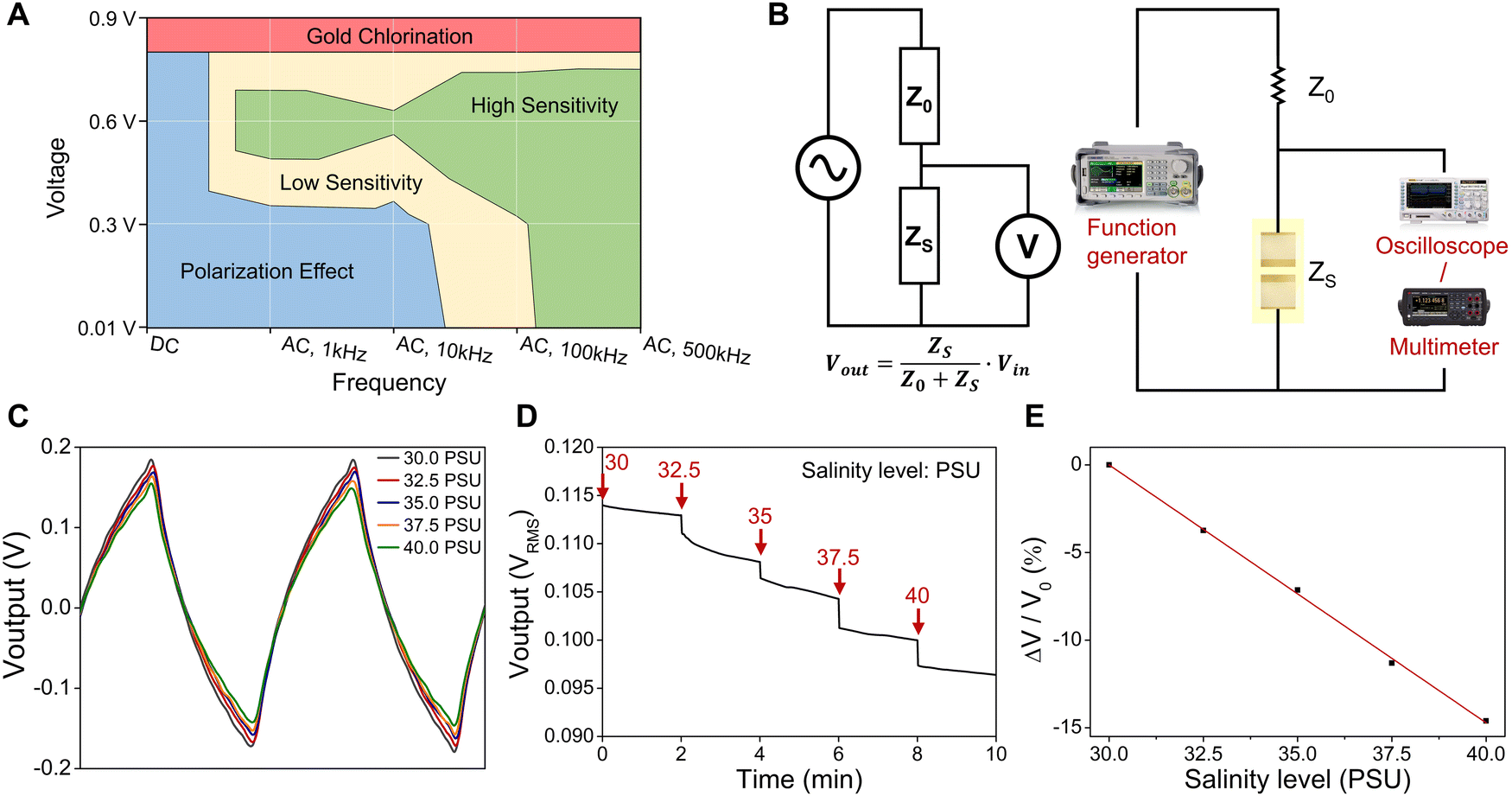 | ||
| Fig. 5 (A) Performance diagram of gold-based salinity sensors operated at various DC/AC voltage and frequencies. (B) Voltage divider circuit and experimental setup for time-dependent salinity measurements. (C) Output AC waveforms of the salinity sensor recorded from an oscilloscope at salinity levels of 30–40 PSU. (D) Time-dependent output voltage (VRMS) recorded from a digital multimeter at salinity levels of 30-40 PSU. (E) Calibration curve of relative output voltage change (ΔV/V0, %) of the salinity sensor as a function of salinity levels. | ||
Furthermore, the performance diagram shows a high sensitivity (green) region representing sensitivity higher than 10% and a low sensitivity (yellow) region with sensitivity values of 5–10%. The sensitivity can be enhanced by using relatively high frequency and voltage to minimize double-layer effects and capacitance contribution to impedance.23,44 In addition to the studies in this work, the performance diagram is also validated in many works. For instance, an Au-electrode conductivity sensor in a sweat collection patch operated at 0.2 Vpp (peak-to-peak voltage) and a frequency of 80 kHz (in the low sensitivity region of the performance diagram) exhibited a conductance sensitivity of 24 μS/mM NaCl when tested in NaCl solutions with a concentration range of 10–150 mM.44 Another Au-electrode impedance-based sweat sensor, which was operated at 100 kHz with an AC signal amplitude of 400 mV (in the high sensitivity region of the performance diagram), possessed an improved conductance sensitivity of approximately 70 μS/mM NaCl calculated from the admittance change when the NaCl concentration varies from 15 to 60 mM.23 The results in this study and those from previous studies effectively validate the performance diagram, which can provide significant guidance for the operation of Au-based electrochemical sensors.
To realize wearable electronic sensor systems for real-time ocean environmental monitoring and data transmission, the salinity sensors need to be integrated with electronics that can offer an AC voltage source and record the impedance changes of salinity sensors for salinity measurement. Here, we demonstrate a proof-of-concept study that utilizes a voltage divider circuit, consisting of an input voltage source and two impedances connected in series, which can create an output voltage that is a fraction of the input voltage. The voltage divide ratio is determined by the two impedances and is given by Voutput = ZS/(Z0 + ZS) × Vinput. Using this basic circuit, the impedance values of salinity sensors at different salinity levels can be converted into output voltage signals for further data processing and recording. In the experimental setup for time-dependent salinity measurements (as described in the experimental section and shown in Fig. 5B), an input of 0.6 VRMS AC (root mean square value of AC voltage) square wave with a frequency of 1 kHz provided by a function generator is applied across a constant resistor (Z0, 20 kΩ) and a salinity sensor (ZS) that are in series. The output voltage signals across the salinity sensor are recorded by an oscilloscope (to record the waveform) and a digital multimeter (to record the voltage). As the salinity level increases from 30 PSU to 40 PSU, the impedance of the salinity sensor decreases, resulting in a decrease in the amplitudes of the output voltage due to the corresponding change in the divide ratio. (Fig. 5C). Please note that the shape of the output waveforms is not the same as that of the input square wave due to the capacitive behavior of the salinity sensor.
The time-dependent output voltage is recorded under salinity levels ranging from 30 PSU to 40 PSU, and the results are shown in Fig. 5D. The output voltage decreases with increasing salinity levels, which is consistent with prior results in Fig. 3 and 4. The output voltage drops to a lower value in 5 seconds and stabilizes at a relatively steady voltage within 2 minutes, which is considered a quick response for the salinity monitoring.30 In addition, the relationship between relative voltage change (ΔV/V0, %) and salinity levels presents a good sensitivity (|ΔV/V0| = ∼15% across 30–40 PSU) and linearity (R2 = 0.99), as shown in Fig. 5E. For future applications, the output voltage signal will be converted to analog-to-digital (ADC) signals and sent to external computing/recording devices via a Bluetooth module for short-distance testing or an acoustic signal transmitter for deep-sea monitoring.
3. Conclusions
In summary, we develop soft, flexible conductivity sensors and systematically study the effect of the magnitude and frequency of operating voltage and exposed sensing areas on the performance of the sensor. We find that an operating voltage lower than the redox potential of the gold chlorination reaction at approximately 0.8 V can effectively eliminate the chloride-induced corrosion and dissolution of gold-based electrochemical sensors. In addition, an AC signal with relatively high amplitude (∼0.6 V) can reduce the polarization effect and provide better sensitivity compared to that under DC signals. A performance diagram is constructed to provide guidance for avoiding gold chlorination and polarization effects and, in the meanwhile, to identify operating voltage and frequency for high sensitivity. The results provide an important guideline for the development of soft metallic-electrode-based electrochemical sensors that can be used for biosensing or hydro-environmental analysis.Moreover, a salinity measurement circuit consisting of a 0.6 V AC voltage source, a voltage divider and a salinity sensor has demonstrated high accuracy and quick response time in real-time salinity monitoring. The future prospect of this work includes incorporating soft salinity sensors with other physical sensors like temperature and pressure sensors into a fully functional multimodal sensing system for real-time CTD (conductivity, temperature, and depth) monitoring of the ocean environments,39 as well as integration with other platforms like soft robotics and diver equipment.
4. Experimental section
Fabrication of soft salinity sensors
The soft salinity sensor comprises a top encapsulation layer (parylene C, 5 μm), a pair of gold (Au, 100 nm) thin-film electrodes (each measuring 4 mm × 4 mm), and parylene C (5 μm)/polyimide (PI, 7.6 μm) substrates. The fabrication processes were reported in our previous work39 and also provided as follows. A layer of PDMS (Sylgard 184, Dow, with an elastomer/curing agent weight ratio of 10:1) was spin-coated onto a glass slide at 1500 rpm for 35 s to enhance the adhesion between the subsequent PI substrate and glass. A 7.6 μm thick PI film was then laminated onto the PDMS-coated glass substrate, and a 5 μm parylene C (Specialty Coating Systems Inc.) layer was deposited on top of the PI film. Next, a bilayer of Au (100 nm)/Cr (10 nm) thin film was deposited onto the parylene C layer using a magnetron sputtering system (AJA Orion-8 Magnetron Sputtering System, AJA International Inc.). The Au/Cr thin film was then patterned into a pair of separated electrodes via photolithography and wet-etching techniques. The patterned sensor electrodes were then encapsulated by depositing a top parylene C layer. To define exposed ion sensing areas for salinity sensors, the top parylene C encapsulation layer was patterned by photolithography processes, followed by reactive ion etching (RIE) with oxygen plasma.
Electrochemical measurement of salinity sensors
Saline solution with salinity levels of 30–40 practical salinity unit (PSU, g kg−1) for all sensor characterizations were prepared by dissolving 30–40 g of NaCl in deionized (DI) water. Electrochemical measurements were performed using a potentiostat/galvanostat instrument (Autolab PGSTAT128N, Metrohm). Linear sweep voltammetry (LSV) was swept from 0 V to 1.5 V at a scan rate of 0.1 V s−1 and a step of 0.01 V. Chronoamperometry applied three steps of voltage (0.2 V, 0.4 V and 0.6 V) and recorded the response current at each step for 1 minute with an interval of 0.1 s. Electrochemical impedance spectroscopy (EIS) was performed in the frequency response analysis (FRA) impedance potentiostatic mode and the response of the sensors was measured by applying a sinusoidal excitation signal (sine wave) with a frequency from 500 kHz to 1 kHz and an amplitude of 0.01 VRMS. The effect of AC voltage and exposed sensing areas on the performance of the salinity sensor were performed using an LCR meter (IM3533, Hioki). The LCR meter recorded the impedance values once per second for 1 min for each test condition. The effect of AC voltage (0.01 V, 0.4 V, 0.6 V and 1.0 V) was tested at a constant frequency of 1 kHz using salinity sensors of the same exposed sensing area (exposed width of 500 μm, denoted as E500). The effect of exposed sensing areas of salinity sensors was tested at a constant frequency of 1 kHz and constant applied VAC of 0.6 V.Voltage divider circuit for time-dependent salinity measurement
A function generator (SDG1032X, Siglent) was used to generate a square wave AC voltage with an amplitude of 0.6 VRMS (root mean square value of AC voltage) and a frequency of 1 kHz. This input voltage was applied across a programmable resistor board set at a constant resistance value of 20 kΩ (Z0) and a salinity sensor (ZS) that were connected in series. The output voltage waveforms across the salinity sensor were captured using an oscilloscope (DS1104Z Plus, Rigol). To test the time-dependent salinity measurement, different concentrations of NaCl were added to the solution to achieve salinity levels of 30–40 PSU. The output AC voltage was continuously measured by a digital multimeter (34470A, Keysight) in VRMS values. The digital multimeter was operated in the data logging mode to record the AC voltage every second.Author contributions
X. W. conceived the idea and supervised the experiments. S. L. conducted the experiments on the fabrication and testing of salinity sensors. Y. L. assisted with the experiments. X. W. and S. L. wrote the manuscript. All authors discussed and commented on the manuscript.Conflicts of interest
There are no conflicts to declare.Acknowledgements
S. L., Y. L., and X. W. would like to acknowledge the support from the Office of Naval Research (N00014-19-1-2688 and N00014-21-1-2342). In addition, this work made use of the maskless aligner μMLA, which was funded by the Defense University Research Instrumentation Program from the Office of Naval Research (N00014-21-1-2223).References
- M. Lin, Z. Zheng, L. Yang, M. Luo, L. Fu, B. Lin and C. Xu, Adv. Mater., 2022, 34, e2107309 CrossRef.
- G. Su, S. Yin, Y. Guo, F. Zhao, Q. Guo, X. Zhang, T. Zhou and G. Yu, Mater. Horiz., 2021, 8, 1795–1804 RSC.
- I. Heck, W. Lu, Z. Wang, X. Zhang, T. Adak, T. Cu, C. Crumley, Y. Zhang and X. S. Wang, Adv. Mater. Technol., 2022, 8, 2200821 CrossRef.
- T. Leelasree, V. Selamneni, T. Akshaya, P. Sahatiya and H. Aggarwal, J. Mater. Chem. B, 2020, 8, 10182–10189 RSC.
- D. H. Keum, S. K. Kim, J. Koo, G. H. Lee, C. Jeon, J. W. Mok, B. H. Mun, K. J. Lee, E. Kamrani, C. K. Joo, S. Shin, J. Y. Sim, D. Myung, S. H. Yun, Z. Bao and S. K. Hahn, Sci. Adv., 2020, 6, eaba3252 CrossRef CAS PubMed.
- Q. Chen, Z. Chen, D. Liu, Z. He and J. Wu, ACS Appl. Mater. Interfaces, 2020, 12, 17713–17724 CrossRef CAS PubMed.
- A. Scidà, S. Haque, E. Treossi, A. Robinson, S. Smerzi, S. Ravesi, S. Borini and V. Palermo, Mater. Today, 2018, 21, 223–230 CrossRef.
- Y. Zhao, B. Wang, H. Hojaiji, Z. Wang, S. Lin, C. Yeung, H. Lin, P. Nguyen, K. Chiu, K. Salahi, X. Cheng, J. Tan, B. A. Cerrillos and S. Emaminejad, Sci. Adv., 2020, 6, eaaz0007 CrossRef CAS.
- Z. Pu, X. Zhang, H. Yu, J. Tu, H. Chen, Y. Liu, X. Su, R. Wang, L. Zhang and D. Li, Sci. Adv., 2021, 7, eabd0199 CrossRef CAS PubMed.
- O. Parlak, S. T. Keene, A. Marais, V. F. Curto and A. Salleo, Sci. Adv., 2018, 4, eaar2904 CrossRef CAS.
- Y. Park, C. K. Franz, H. Ryu, H. Luan, K. Y. Cotton, J. U. Kim, T. S. Chung, S. Zhao, A. Vazquez-Guardado, D. S. Yang, K. Li, R. Avila, J. K. Phillips, M. J. Quezada, H. Jang, S. S. Kwak, S. M. Won, K. Kwon, H. Jeong, A. J. Bandodkar, M. Han, H. Zhao, G. R. Osher, H. Wang, K. Lee, Y. Zhang, Y. Huang, J. D. Finan and J. A. Rogers, Sci. Adv., 2021, 7, eabf9153 CrossRef CAS.
- S. H. Ko, S. W. Kim and Y. J. Lee, Sci. Rep., 2021, 11, 21101 CrossRef.
- R. Hajian, S. Balderston, T. Tran, T. deBoer, J. Etienne, M. Sandhu, N. A. Wauford, J. Y. Chung, J. Nokes, M. Athaiya, J. Paredes, R. Peytavi, B. Goldsmith, N. Murthy, I. M. Conboy and K. Aran, Nat. Biomed. Eng., 2019, 3, 427–437 CrossRef CAS.
- J. Sabate Del Rio, H. K. Woo, J. Park, H. K. Ha, J. R. Kim and Y. K. Cho, Adv. Mater., 2022, 34, e2200981 CrossRef.
- H. Liu, A. Yang, J. Song, N. Wang, P. Lam, Y. Li, H. K. Law and F. Yan, Sci. Adv., 2021, 7, eabg8387 CrossRef CAS PubMed.
- Y. Gao, D. T. Nguyen, T. Yeo, S. B. Lim, W. X. Tan, L. E. Madden, L. Jin, J. Y. K. Long, F. A. B. Aloweni, Y. J. A. Liew, M. L. L. Tan, S. Y. Ang, S. D. Maniya, I. Abdelwahab, K. P. Loh, C. H. Chen, D. L. Becker, D. Leavesley, J. S. Ho and C. T. Lim, Sci. Adv., 2021, 7, eabg9614 CrossRef CAS.
- R. Li, H. Qi, Y. Ma, Y. Deng, S. Liu, Y. Jie, J. Jing, J. He, X. Zhang, L. Wheatley, C. Huang, X. Sheng, M. Zhang and L. Yin, Nat. Commun., 2020, 11, 3207 CrossRef CAS PubMed.
- M. Ku, J. Kim, J. E. Won, W. Kang, Y. G. Park, J. Park, J. H. Lee, J. Cheon, H. H. Lee and J. U. Park, Sci. Adv., 2020, 6, eabb2891 CrossRef CAS PubMed.
- H. P. Phan, Y. Zhong, T. K. Nguyen, Y. Park, T. Dinh, E. Song, R. K. Vadivelu, M. K. Masud, J. Li, M. J. A. Shiddiky, D. Dao, Y. Yamauchi, J. A. Rogers and N. T. Nguyen, ACS Nano, 2019, 13, 11572–11581 CrossRef CAS PubMed.
- H. Lee, C. Song, Y. S. Hong, M. Kim, H. R. Cho, T. Kang, K. Shin, S. H. Choi, T. Hyeon and D. H. Kim, Sci. Adv., 2017, 3, e1601314 CrossRef PubMed.
- J. Xu, Z. Zhang, S. Gan, H. Gao, H. Kong, Z. Song, X. Ge, Y. Bao and L. Niu, ACS Sens., 2020, 5, 2834–2842 CrossRef CAS.
- Y. Song, J. Min, Y. Yu, H. Wang, Y. Yang, H. Zhang and W. Gao, Sci. Adv., 2020, 6, eaay9842 CrossRef CAS.
- H. Y. Y. Nyein, L.-C. Tai, Q. P. Ngo, M. Chao, G. B. Zhang, W. Gao, M. Bariya, J. Bullock, H. Kim, H. M. Fahad and A. Javey, ACS Sens., 2018, 3, 944–952 CrossRef CAS PubMed.
- Y. H. Kim, K. Lee, H. Jung, H. K. Kang, J. Jo, I. K. Park and H. H. Lee, Biosens. Bioelectron., 2017, 98, 473–477 CrossRef CAS PubMed.
- P. K. Vabbina, A. Kaushik, N. Pokhrel, S. Bhansali and N. Pala, Biosens. Bioelectron., 2015, 63, 124–130 CrossRef CAS PubMed.
- H. Teymourian, C. Moonla, F. Tehrani, E. Vargas, R. Aghavali, A. Barfidokht, T. Tangkuaram, P. P. Mercier, E. Dassau and J. Wang, Anal. Chem., 2020, 92, 2291–2300 CrossRef CAS PubMed.
- S. F. Shaikh, H. F. Mazo-Mantilla, N. Qaiser, S. M. Khan, J. M. Nassar, N. R. Geraldi, C. M. Duarte and M. M. Hussain, Small, 2019, 15, e1804385 CrossRef PubMed.
- A. Kaidarova, M. A. Khan, M. Marengo, L. Swanepoel, A. Przybysz, C. Muller, A. Fahlman, U. Buttner, N. R. Geraldi, R. P. Wilson, C. M. Duarte and J. Kosel, npj Flexible Electron., 2019, 3, 15 CrossRef.
- A. Kaidaorva, M. Marengo, G. Marinaro, N. R. Geraldi, R. Wilson, C. M. Duarte and J. Kosel, Results Mater., 2019, 1, 100009 CrossRef.
- J. M. Nassar, S. M. Khan, S. J. Velling, A. Diaz-Gaxiola, S. F. Shaikh, N. R. Geraldi, G. A. Torres Sevilla, C. M. Duarte and M. M. Hussain, npj Flexible Electron., 2018, 2, 13 CrossRef.
- F. Akhter, H. R. Siddiquei, M. E. E. Alahi, K. P. Jayasundera and S. C. Mukhopadhyay, IEEE Internet Things J., 2022, 9, 14307–14316 Search PubMed.
- M. Chen, M. Zhang, X. Wang, Q. Yang, M. Wang, G. Liu and L. Yao, Sensors, 2020, 20, 2270 CrossRef CAS.
- Y. Sui and C. A. Zorman, J. Electrochem. Soc., 2020, 167, 037571 CrossRef CAS.
- J. Li, E. Song, C. H. Chiang, K. J. Yu, J. Koo, H. Du, Y. Zhong, M. Hill, C. Wang, J. Zhang, Y. Chen, L. Tian, Y. Zhong, G. Fang, J. Viventi and J. A. Rogers, Proc. Natl. Acad. Sci. U. S. A., 2018, 115, E9542–E9549 CAS.
- O. Kasian, N. Kulyk, A. Mingers, A. R. Zeradjanin, K. J. J. Mayrhofer and S. Cherevko, Electrochim. Acta, 2016, 222, 1056–1063 CrossRef CAS.
- H. A. Rahman, S. W. Harun, M. Yasin, S. W. Phang, S. S. A. Damanhuri, H. Arof and H. Ahmad, Sens. Actuators, A, 2011, 171, 219–222 CrossRef CAS.
- I. Hussain, M. Das, K. U. Ahamad and P. Nath, Sens. Actuators, B, 2017, 239, 1042–1050 CrossRef CAS.
- N. Ali, J. A. Teixeira, A. Addali, M. Saeed, F. Al-Zubi, A. Sedaghat and H. Bahzad, Materials, 2019, 12, 571 CrossRef CAS PubMed.
- Y. Li, G. Wu, G. Song, S. H. Lu, Z. Wang, H. Sun, Y. Zhang and X. Wang, ACS Sens., 2022, 7, 2400–2409 CrossRef CAS PubMed.
- A. Kaidarova, M. Marengo, G. Marinaro, N. Geraldi, C. M. Duarte and J. Kosel, Adv. Mater. Interfaces, 2018, 5, 1801110 CrossRef.
- G. H. Kelsall, N. J. Welham and M. A. Diaz, J. Electroanal. Chem., 1993, 361, 13–24 CrossRef CAS.
- J. Park, W.-M. Choi, K. Kim, W.-I. Jeong, J.-B. Seo and I. Park, Sci. Rep., 2018, 8, 264 CrossRef.
- B. You, Y. Yue, M. Sun, J. Li and D. Jia, Sensors, 2021, 21, 3086 CrossRef CAS.
- A. S. M. Steijlen, K. M. B. Jansen, J. Bastemeijer, P. J. French and A. Bossche, Anal. Chem., 2022, 94, 6893–6901 CrossRef CAS.
Footnote |
| † Electronic supplementary information (ESI) available. See DOI: https://doi.org/10.1039/d3tb01167d |
| This journal is © The Royal Society of Chemistry 2023 |