
Computational design of self-assembling peptide chassis materials for synthetic cells†
Yutao
Ma
a,
Rohan
Kapoor
a,
Bineet
Sharma‡
 b,
Allen P.
Liu
bcde and
Andrew L.
Ferguson
*a
b,
Allen P.
Liu
bcde and
Andrew L.
Ferguson
*a
aPritzker School of Molecular Engineering, University of Chicago, Chicago, Illinois 60637, USA. E-mail: andrewferguson@uchicago.edu; Tel: +1 773 7025950
bDepartment of Mechanical Engineering, University of Michigan, Ann Arbor, Michigan 48109, USA
cDepartment of Biomedical Engineering, University of Michigan, Ann Arbor, Michigan 48109, USA
dCellular and Molecular Biology Program, University of Michigan, Ann Arbor, Michigan 48105, USA
eDepartment of Biophysics, University of Michigan, Ann Arbor, Michigan 48105, USA
First published on 22nd September 2022
Abstract
Giant lipid vesicles have been used extensively as a synthetic cell model to recapitulate various life-like processes, including in vitro protein synthesis, DNA replication, and cytoskeleton organization. Cell-sized lipid vesicles are mechanically fragile in nature and prone to rupture due to osmotic stress, which limits their usability. Recently, peptide vesicles have been introduced as an alternative chassis material for synthetic cells that are more robust and stable than lipid vesicles, and can withstand harsh conditions including pH, thermal, and osmotic variations. In this work, we combine coarse-grained molecular simulation, enhanced sampling free energy calculations, Gaussian process regression, and Bayesian optimization to construct an active learning screening for diblock amphiphilic elastin-like polypeptides capable of forming thermodynamically stable vesicular structures suitable for the self-assembly of synthetic peptide vesicles. Our computational screen identifies a number of promising sequences that form peptidic vesicles with high thermodynamic stabilities relative to isolated peptides in bulk solvent on the order of 10–15kBT per amino acid residue.
Design, System, ApplicationPeptides have become a popular class of building blocks for self-assembly due to their versatility and modulability. In this work, we combined coarse-grained simulations, free energy calculations, and black-box optimization algorithms to develop a high-throughput screening protocol to discover optimal diblock amphiphilic elastin-like polypeptides that could self-assemble into stable vesicles. We performed molecular dynamics and enhanced sampling simulations to quantify the thermodynamic stability of the vesicle formed by the polypeptides, trained Gaussian process regression surrogate models to relate polypeptide sequence to vesicle stability, and Bayesian optimization to rationally traverse the polypeptide design space to efficiently identify peptides that maximize vesicle stability. Self-assembling peptidic vesicles can serve as promising chassis materials for synthetic cells which have a wide range of applications in drug delivery and biosensing. Our high-throughput screening protocol could be extended to other self-assembling peptides or proteins to optimize the amino acid sequence for particular structural or functional goals. |
1 Introduction
Synthetic cells are engineered biological or polymeric membranes that mimic one or many functions of a biological cell. They have a wide range of applications, ranging from fundamental knowledge such as the origin of life to applied nanotechnology such as smart drug delivery and biosensors.1,2 Generally speaking, there are two routes to manufacture synthetic cells: the “top-down” approach and the “bottom-up” approach.3 The former approach mainly focuses on simplifying existing living cells to obtain minimal cells, while the latter approach tries to synthesize artificial cells by assembling from nonliving building blocks.3 Recently, the bottom-up approach has drawn substantial research interest.4,5 Lipids have been the natural and most widely used building blocks for synthetic cells6 due to the similarity of lipid bilayers (liposomes) to natural biological membranes.2 However, cell-sized lipid vesicles are mechanically fragile and sensitive to chemical stress (e.g., oxidation) and osmotic pressure.7,8 Opportunities exist to explore alternative and more robust chassis materials for synthetic cell membranes. Polymersomes constructed from diblock copolymers were one of the earliest non-lipid building blocks demonstrated as synthetic vesicles9 and novel molecules with improved materials properties exploiting new synthetic polymers continue to be developed.10 A drawback of polymersomes is that they are typically constituted from artificial monomers that can have limited biocompatibility and therefore compromise the integration of the synthetic cell with other components of the biological milieu.Elastin-like polypeptides (ELPs) have recently been demonstrated as a structurally robust and biocompatible chassis material for synthetic cells11,12 that can form ∼50 nm diameter unilamellar vesicles13 and can be templated to form giant vesicles with diameters in excess of 50 μm.14 ELPs are synthetic biopolymers that share structural characteristics with intrinsically disordered proteins such as tropoelastin. The general motif of ELP polymers is a pentapeptide repeat (VPGXG)n, where V is valine, P is proline, G is glycine and X can be any guest residue except proline. ELPs are intrinsically disordered polymers that exhibit temperature-triggered phase transition: below a lower critical solution temperature (LCST) the ELP adopts a random coil configuration, while above the LCST the ELP undergoes and ordering transition into β-spiral secondary structures constituted of type II β-turns.15,16 The guest residue X has a strong influence upon the LCST, where the LCST typically decreases as the hydrophobicity of the guest residue increases; proline cannot be used as a guest residue as it compromises the LCST behavior.15,17,18 Amphiphilic diblock and multiblock ELPs have drawn particular interest because their temperature-dependent ordering and self-assembly behavior can be manipulated by controlling the guest residues in each block. Micelles are the most common self-assembled structures from amphiphilic diblock ELPs, where the hydrophobic block has the lower LCST Tlo and the hydrophilic block has the higher LCST Thi. At Tlo < T < Thi, the hydrophobic blocks associate with each other to form the core of the micelles while the hydrophilic blocks form the corona.19 However, several recent experiments have indicated that amphiphilic diblock and triblock ELPs could self-assemble into large vesicular structures that are stable under harsh conditions such as extremes of pH or temperature.20 For example, Vogele et al. have utilized glass bead method to direct a diblock ELP with glutamic acid as the hydrophilic guest residue and phenylalanine as the hydrophobic guest residue to form giant vesicles.11 Schreiber et al. compared the vesicular structures formed by two kinds of diblock ELPs with the same lengths but different guest residues and concluded that guest residue composition could be a key factor in modulating the vesicle stability.21 Frank et al. demonstrated the formation of giant ELP vesicles by using solvent evaporation method.22 Very recently, we demonstrated the production of giant (>50 μm) vesicles from amphiphilic ELP diblocks using emulsion transfer techniques.14
The vast number of potential amphiphilic ELP diblock sequences means that principled approaches are required to efficiently traverse and optimize within this design space. Consider the space defined by the sequence (VPGX1G)m(VPGX2G)n, where X1 is one of twelve hydrophilic amino acid residues (except proline) categorized under the Kyte–Doolittle hydropathy scale23 {G, T, S, W, Y, H, E, Q, D, N, K, R}, X2 is one of seven hydrophobic residues {I, V, L, F, C, M, A}, and the degree of the hydrophilic m and hydrophobic n repeats can vary over the range 5–100, this defines a design space of 12 × 7 × 96 × 96 = 774![[thin space (1/6-em)]](https://www.rsc.org/images/entities/char_2009.gif) 144 possible sequences. The engineering of amphiphilic diblock ELPs for vesicle formation is generally conducted using chemical intuition to specify the identity of the guest residues and the lengths of the hydrophilic and hydrophobic blocks. Opportunities exist to systematize and accelerate this search using data-driven and model-guided approaches to efficiently identify sequences capable of forming stable vesicle structures and simultaneously develop fundamental understanding and design rules linking the ELP sequence to the emergent vesicle stability. Machine learning techniques such as kernel regression,24,25 support vector machines (SVM),26 and artificial neural networks,27 have provided useful tools for the prediction of chemical or physical properties of soft materials and the discovery of novel materials with specific functionalities. For example, Leslie et al. proposed a string kernel based on a tree data structure to perform SVM classification of proteins for several benchmark tasks.28 Lee et al. used SVMs to identify and discover new membrane-active and antimicrobial α-helical peptides.29 Zhou et al. used Gaussian process regression model with custom kernel to predict the antimicrobial abilities of various pentadecapeptides.24 Lei et al. built a deep learning framework based on convolutional neural networks to predict peptide–protein interactions.30 Mohr et al. trained a regularized autoencoder to embed small organic molecules onto a latent space and perform Bayesian optimization over the latent space to discover molecules capable of permeating cardiolipin-containing membranes.31 In general, machine learning techniques are powerful tools that can assist the discovery of novel functional materials by learning predictive or generative models from computational and/or experimental data.
144 possible sequences. The engineering of amphiphilic diblock ELPs for vesicle formation is generally conducted using chemical intuition to specify the identity of the guest residues and the lengths of the hydrophilic and hydrophobic blocks. Opportunities exist to systematize and accelerate this search using data-driven and model-guided approaches to efficiently identify sequences capable of forming stable vesicle structures and simultaneously develop fundamental understanding and design rules linking the ELP sequence to the emergent vesicle stability. Machine learning techniques such as kernel regression,24,25 support vector machines (SVM),26 and artificial neural networks,27 have provided useful tools for the prediction of chemical or physical properties of soft materials and the discovery of novel materials with specific functionalities. For example, Leslie et al. proposed a string kernel based on a tree data structure to perform SVM classification of proteins for several benchmark tasks.28 Lee et al. used SVMs to identify and discover new membrane-active and antimicrobial α-helical peptides.29 Zhou et al. used Gaussian process regression model with custom kernel to predict the antimicrobial abilities of various pentadecapeptides.24 Lei et al. built a deep learning framework based on convolutional neural networks to predict peptide–protein interactions.30 Mohr et al. trained a regularized autoencoder to embed small organic molecules onto a latent space and perform Bayesian optimization over the latent space to discover molecules capable of permeating cardiolipin-containing membranes.31 In general, machine learning techniques are powerful tools that can assist the discovery of novel functional materials by learning predictive or generative models from computational and/or experimental data.
In this work, we propose a high-throughput screening protocol that combines coarse-grained molecular dynamics simulation, enhanced sampling free energy calculations, Gaussian process regression (GPR), and Bayesian optimization (BO) to discover optimal peptides from a library of diblock amphiphilic ELPs that could form vesicular structures with high thermodynamic stability. Our screening efficiently identifies high-performing ELP sequences as good candidates for the formation of stable synthetic cell membranes, furnishes a predictive model linking ELP sequence to thermodynamic stability and provides a filtration of the vast ELP design space to identify the top candidates for experimental testing. Our computational screen is approximately 15× faster than experimental assessment of the ELP candidates, presenting a relatively higher throughput means to prospectively identify the top performing candidates for future experimental testing. The high-throughput screening protocol can be straightforwardly extended to the design of multiblock ELPs32 or ELP conjugates with other biopolymers such as collagen-like polypeptides.33,34 More generally, the approach can be applied to the design and optimization of polypeptide sequences with other desired structural or functional properties measured by computational and/or experimental assays.
2 Methods
2.1 Molecular modeling of ELP vesicles
The objective of our molecular modeling calculations is to furnish computational estimates for the thermodynamic stability of vesicles formed from diblock amphiphilic ELPs. We assume that the vesicles are pre-assembled using experimental techniques such as solvent evaporation22,35 or emulsion transfer.14 An entire vesicle with a diameter of microns or more12,14 is extremely expensive to simulate in its entirety. Instead we focus on a zoomed-in region of the vesicle wall that can be accurately approximated as a planar bilayer and simulated by classical molecular dynamics (Fig. 1).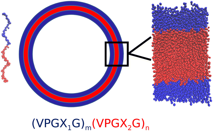 | ||
| Fig. 1 Illustration of an amphiphilic diblock ELP molecule (left) and bilayer vesicle (right). The hydrophobic block is shown in red and the hydrophilic block is shown in blue. The bilayer wall is locally well approximated as a planar sheet (inset). (VPGX1G)m(VPGX2G)n denotes the sequence of a generic amphiphilic diblock ELP, where X1 is a hydrophilic guest amino acid residue, X2 is a hydrophobic guest amino acid residue, and m and n are the degree of hydrophilic block and hydrophobic repeats. | ||
All-atom representations of ELP molecules (VPGX1G)m(VPGX2G)n were constructed using PyMol36 and then coarse grained using the Martini force field version 2.2.37 We employ a coarse-grained modeling approach in order to allow us to reach the length scales necessary to model a substantial patch of the bilayer wall and the time scales needed to converge the free energy calculations (see section 2.2) by which we estimate bilayer stability. A limitation of the Martini force field is that it requires specification of the secondary structure of each region of a protein. As such, changes in secondary structure cannot be modeled over the course of the simulation, although changes in the tertiary structure are, within this approximation, accurately treated.38 For each system we assume that the LCST of the hydrophobic block Tlo lies below the ambient temperature T and therefore model the secondary structure of this block as a β-turn, whereas the LCST of the hydrophilic block Thi lies above the ambient temperature and is therefore modeled as a random coil.15,16 The precise LCSTs of various ELPs are not precisely known, so we simply conduct all of our calculations at T = 300 K and P = 1 bar under these secondary structure assumptions. This carries the benefit of enabling us to compute thermodynamic stabilities at a consistent thermodynamic state point without requiring knowledge of the LCSTs but is a significant assumption that we are impelled to make due to the absence of comprehensive LCST data for all ELP sequences and the secondary structure limitations of the Martini model. Although we do not do so here, we suggest two possible strategies to relax this assumption. First, one may consider employing all-atom simulations to estimate the LCSTs and then use this information to conduct simulations at Tlo < T < Thi. The computational burden to do so is quite high, but would lead to a more accurate coarse-grained simulation protocol. Second, one could consider employing an alternative coarse-grained model that does not require specification of secondary structure such as the SIRAH force field.39,40 In the present work, we assume that the trends in the thermodynamic stabilities calculated under our simplifying assumptions still serve as a useful ranking and filtration of ELP sequences predicted to form stable vesicles. As discussed below, post hoc validation of our protocol is provided by its identification of a top-ranked candidate that has been experimentally demonstrated form stable vesicles with lifetime of several hours.
We model an approximately 81 nm2 patch of the vesicle wall by constructing a 10 × 10 grid of fully extended amphiphilic diblock ELP chains separated in x and y directions by 0.9 nm to create the upper leaflet and another 10 × 10 grid of ELP chains to create the lower leaflet. The ELP chains in the lower leaflet were flipped upside down so that the hydrophobic blocks of these two layers lie adjacent to one another to form the hydrophobic core of the bilayer sandwich. We then solvated the bilayer patch comprising the 200 ELP chains by adding non-polarizable Martini water molecules41 at a density of 1 g cm−3 up to a distance of 34.5 nm above and 10 nm below the x–y plane of the bilayer. When creating topology, we set the solvent-exposed N-terminus to be positively charged (corresponding to VAL-NH3+) and the C-terminus buried within the solvent-excluded hydrophobic core of the bilayer to be neutral (corresponding to GLY-COOH).42 Ionization states of amino acid sidechains were specified with the most prevalent protonation state at pH 7. All guest residues in the hydrophobic X2 position are electrically neutral. A subset of those in the hydrophilic X1 position adopt charged states: {E: (−1), D: (−1), K: (+1), R: (+1)}. Where necessary, a number of monovalent Martini counterions, employing Qa beads for Cl− ions and Qd beads for Na+ ions, were randomly inserted into the water region in order to maintain charge neutrality. This initial state of the system exists in a 9 × 9 × 67 nm3 box with periodic boundary conditions applied in all three dimensions. The z-dimension of the box was chosen to be sufficiently large to provide an initial linear separation of 44.5 nm between the upper and lower leaflets of the bilayer through the periodic wall in z, thereby effectively eliminating direct interactions between periodic images of the bilayer, minimizing any artifacts associated with the periodic boundary conditions and enabling us to conduct the chain extraction free energy calculations detailed in section 2.2. An illustration of the initial bilayer setup is presented in Fig. 2a.
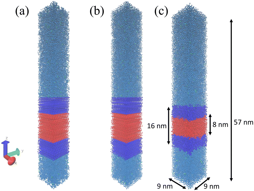 | ||
| Fig. 2 Illustration of (a) initial bilayer, (b) bilayer after energy minimization and (c) relaxed bilayer after NPT production run. The dark blue beads represent hydrophilic blocks, the red beads represent hydrophobic blocks, the light blue beads are coarse-grained water, and the green beads are negatively-charged monovalent ions. The dimension of the bilayer after NPT production run is also marked. | ||
After setting up the initial bilayer, we first ran steepest descent energy minimization to eliminate forces in excess of 1000 kJ mol−1 nm−1 (Fig. 2b), followed by assignment of initial atom velocities from a Maxwell–Boltzmann distribution at 300 K, then a 10 ns NVT equilibration simulation at 300 K followed by a 10 ns NPT equilibration simulation at 300 K and 1 bar to allow relaxation of the extended ELPs. Finally, we performed 200 ns NPT production runs at 300 K and 1 bar after which the energy, temperature, pressure, and structure all attained stable values allowing the bilayer to attain its equilibrium configuration and place the system into a relaxed state for the enhanced sampling free energy calculations (Fig. 2c). We also confirmed that the density profiles of the solvent and bilayer no longer changed during the 200 ns simulation. For all simulations, the temperature was controlled by a stochastic velocity re-scaling thermostat with a time constant of 1 ps.43 For NPT equilibration runs we employed a Berendsen barostat44 with a time constant of 12 ps and a compressibility of 3 × 10⁻⁴ bar−1. For the NPT production runs we used a Parrinello–Rahman barostat45 with a time constant of 12 ps and a compressibility of 3 × 10⁻⁴ bar−1. In all cases we employed semi-isotropic pressure coupling, which was isotropic in x and y directions (in-plane of bilayer) but decoupled from z (normal to bilayer). The step size for all simulations was set to 20 fs and equations of motion were integrated using the leap-frog scheme.46 Lennard-Jones interactions were smoothly shifted to zero at a cutoff of 1.1 nm. Electrostatics were treated using the reaction field method with εrf = ∞ and εr = 15, as appropriate for the non-polarizable water model.41 All molecular dynamics simulations were performed using the Gromacs 2019 simulation suite.47 Calculations were performed on 10 × 2.40 GHz Intel Xeon Gold 6148 CPU cores and one NVIDIA TITAN V GPU, achieving execution speeds of ∼4.2 μs per day. Simulation trajectories were visualized using VMD.48 The input files required to perform each stage of the simulations are provided in the Github repository available at https://github.com/tommayutao/ELP-Screening.
2.2 Enhanced sampling free energy calculations of ELP vesicle stability
We measure the thermodynamic stability of the vesicle formed by a particular ELP by using enhanced sampling free energy calculations to estimate the free energy change ΔG for insertion of a single ELP molecule into the bilayer (Fig. 3). Thermodynamically, this calculation measures the reversible free energy change associated with the association process (N − 1) + 1 ⇌ N, where in the present case N = 200 ELP chains constitute the assembled bilayer. Physically, it measures the free energy change to introduce a single ELP from bulk solvent into the bilayer. Since our objective is to maximize the thermodynamic stability of the ELP vesicle, we wish to identify ELP sequences that make the free energy cost of this insertion process as favorable (i.e., large and negative) as possible. We assume that the free energy difference for the extraction of a single molecule is a good proxy measure for the thermodynamic stability of the bilayer and, by extension, entire vesicle. Lemkul and Bevan have performed molecular dynamics simulation to determine the PMF of extracting constituent peptide from Alzheimer's amyloid protofibril to assess the stabilities of these fibrils.49 Sevgen et al. used similar technique to estimate the stability of micelles formed by block copolymers composed of oligo(ethylene sulfide) and poly(ethylene glycol) blocks.50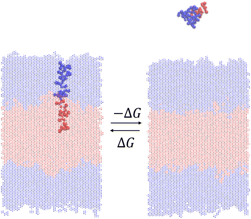 | ||
| Fig. 3 Illustration of the free energy of association ΔG that is equal and opposite to the free energy of dissociation (−ΔG). The single ELP chain extracted from the bilayer is highlighted in solid color and the remaining 199 chains constituting the bilayer are made transparent. Solvent and counterions are omitted for clarity. | ||
We estimate ΔG by computing the potential of mean force (PMF) of the dissociation process N → (N − 1) + 1 along a reversible pathway connecting the associated and dissociated states. Since the path is reversible, it is of course possible to also compute this quantity along the association pathway, but it is more challenging to construct a path to efficiently insert and relax the incoming peptide within the bilayer than to extract a peptide from a pre-assembled bilayer. The free energy difference between the start and end of this path provides an estimate of ΔG.
Due to the possible existence of many local free energy minima that the system could be trapped in, enhanced sampling techniques are usually used to facilitate sufficient sampling of all relevant configurations to ensure good estimate of free energy profile.51 There exist many techniques to perform enhanced sampling, including metadynamics,52 adaptive biasing force53 and umbrella sampling.54 Trajectories produced by enhanced sampling methods that introduce artificial biasing forces to help the system escape local free energy minima must be post-processed to obtain unbiased estimates of the PMF, and various analysis techniques such as multistate Bennett acceptance ratio (MBAR)55 and weighted histogram analysis method (WHAM)56–58 have been proposed to perform that task. In this work, we use a combination of umbrella sampling and WHAM to estimate the unbiased PMF.
After creating and equilibrating the ELP bilayer as detailed in section 2.1, we randomly chose a peptide chain from the upper bilayer for extraction. We extract the chain to effect the dissociation process N → (N − 1) + 1 by constructing a reversible pathway through a space spanned by the two collective variables zhead and ztail (Fig. 4a). zhead is the z-component of the displacement from the center of mass (COM) of the bilayer to the COM of hydrophilic block of chosen chain and ztail is the z-component of displacement from the COM of the bilayer to the COM of hydrophobic block of the chosen chain. The pulling process was divided into three stages (Fig. 4b).
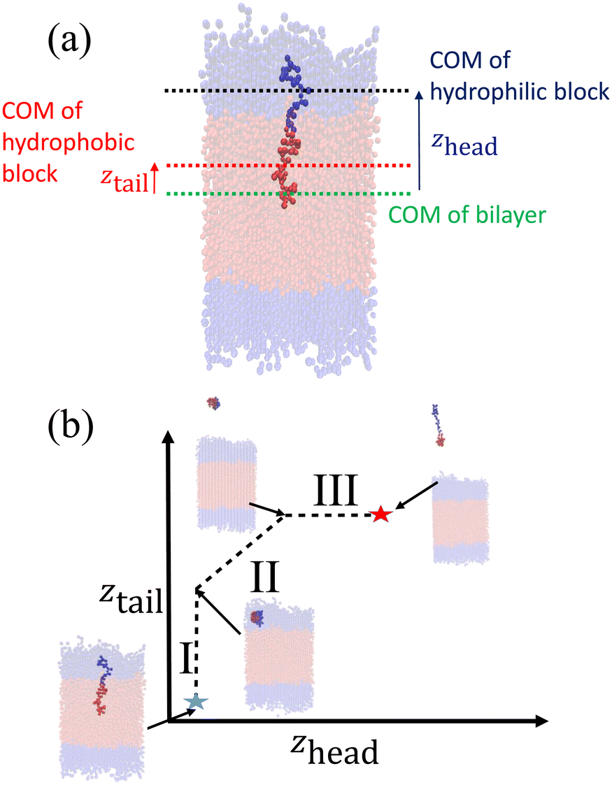 | ||
| Fig. 4 Illustration of umbrella sampling collective variables and construction of the reversible pulling pathway. (a) Definition of zhead and ztail. (b) Schematic illustration of the three components of the reversible pulling pathway in (zhead, ztail) space over which the PMF is constructed. | ||
In stage I, the lower hydrophobic block of the chain is pulled upwards into the upper hydrophilic components of the bilayer. This pathway is generated by constructing a set of overlapping umbrella potentials in (zhead, ztail) space in which zhead = 4.81 nm is fixed to its initial value using a harmonic spring and ztail = [1.21, 5.57] nm is subjected to harmonic restraints with progressively increasing z values in each successive umbrella window to chart a vertical path in (zhead, ztail) space (the precise value of zhead and range of ztail depends on the sequence in question, so here and below we report representative values for the (VPGYG)5(VPGCG)4 sequence). The free energy change associated with the first stage is large and positive due primarily to a large unfavorable enthalpy associated with moving the hydrophobic block of the chain from a hydrophobic to a hydrophilic environment.
In stage II, the chain is extracted from the upper hydrophilic portion of the bilayer into the bulk solvent. We achieve this by laying down a set of umbrella windows with progressively increasing values of zhead = [4.86, 11.86] nm and ztail = [5.48, 12.48] nm that move in lock step to chart out a diagonal path in (zhead, ztail) space. After much trial-and-improvement, we found that extracting the chain from the bilayer in a collapsed configuration – as opposed to simpler approaches of, for example, just pulling on the chain COM or pulling first the head and then the tail – helps prevent snagging of the pulled chain on loops formed by other chains in the bilayer, avoid strong hysteresis effects associated with overextension and rapid relaxation as the chain tail exits the bilayer, and achieve good equilibration and overlap between successive umbrella windows. The free energy change associated with the second stage is also large and positive due primarily to the loss of favorable enthalpic interactions between the extracted chain and the other chains in the bilayer. We ensure that the chain is removed sufficiently far from the top of the bilayer that we observe a plateau in the free energy profile indicating that there are no longer any direct interactions between the pulled chain and the bilayer and that the chain can be approximated to exist in bulk solvent. A sufficiently large z-dimension of the simulation box is critical to enable us to reach this regime before the pulled chain begins interacting with the opposing leaflet of the bilayer through the periodic boundary.
In stage III, the hydrophobic tail is fixed in place and the hydrophilic head pulled away from it to extend the chain out in bulk solvent. We achieve this by constructing a horizontal pathway of umbrella windows in (zhead, ztail) space wherein in each window ztail = 12.47 nm is held at the same value taken on at the end of the second stage and zhead = [11.86, 15.85] nm is subjected to harmonic restraints with progressively increasing z values in each successive umbrella window. The purpose of the last stage is to allow the peptide chain to relax to its equilibrium chain length in bulk solvent and we terminate this stage after we observe a local minimum in the free energy profile. The free energy change associated with chain relaxation in the third stage is small and negative.
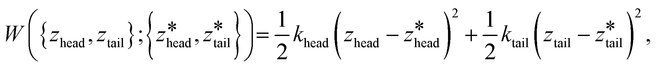
We employed 144, 145, and 28 equally spaced umbrella windows in each of stages I, II, and III, respectively, where the values of zhead and ztail in each window were subjected to harmonic restraints of the form,
 | (1) |
 are the centers for the harmonic potential and {khead, ktail} are the harmonic spring constants. We employed spring constants in the range khead = [1000, 12000] kJ mol−1 nm−2 and ktail = [1000, 20000] kJ mol−1 nm−2. We fine-tuned the spacing between adjacent umbrella windows and the strength of harmonic constraints to ensure good overlaps of histograms from each umbrella sampling simulation. Stiffer springs were typically required within the bilayer (stage I and early stage II) relative to bulk solvent (later stage II and stage III) in order to achieve converged sampling around the centers of the harmonic potential.
Initial configurations for each umbrella window were generated by non-equilibrium pulling simulations conducted as follows. In stage I, spring constants of khead = ktail = 15000 kJ mol−1 nm−2 were applied to a chain initially embedded in the bilayer and the harmonic center  was fixed at the starting value of zhead.
  was gradually increased from the starting value with a rate of 5 × 10⁻⁵ nm ps−1 until it reached
  . In stage II pulling, both spring constants were set to 20000 kJ mol−1 nm−2 and both harmonic centers were increased from their starting values with a rate of 5 × 10⁻⁵ nm ps−1 until the chain left the upper layer. In stage III pulling, both spring constants were set to 5000 kJ mol−1 nm−2.
  was kept fixed at the starting value of ztail and
  was increased from the starting value with a rate of 5 × 10⁻⁵ nm ps−1 for 80 ns. In all pulling simulations, temperature was controlled by stochastic velocity re-scaling and pressure was controlled by Parrinello–Rahman barostat. For each umbrella window centered on
  , the configuration along the non-equilibrium pulling path closest in (zhead, ztail) was selected as the initial configuration.
In each umbrella sampling simulation, we first performed 40 ns NPT equilibration with stochastic velocity re-scaling thermostat and Berendsen barostat followed by a 100 ns production run with stochastic velocity re-scaling thermostat and Parrinello–Rahman barostat. All other simulation parameters were specified as detailed above. Simulations were performed using Gromacs 2019 (ref. 47) and the WHAM analysis was conducted using the program developed in Grossfield Lab61 to reconstruct the unbiased PMF in (zhead, ztail) collective variable space.
The free energy of association ΔG is taken as the difference between the global free energy minimum when the peptide chain is embedded in the bilayer within stage I and the local minimum free energy of the chain in bulk solvent within stage III. Uncertainties in ΔG were estimated by five-fold block averaging. We also note that the chain in bulk solvent is still harmonically restrained in the z-dimension and we can analytically estimate the free energy change associated with the release of these constraints and the COM translational entropy gain associated with the chain exploring the free volume accessible to it at a standard concentration of 1 mol L−1.62–64 To do this, we assume an effective harmonic constraint on zCOM, the z-component of the displacement from the COM of bilayer to the COM of the entire pulled chain, when the pulled chain exists in bulk solvent. We estimate the spring constant Kr of the effective harmonic restraint by collecting histograms of zCOM from the equilibrated portions of all umbrella sampling windows within bulk solvent, fit Gaussian distributions to each of these histograms, estimate the spring constants from the standard deviations of a Gaussian fit, and take the mean as our estimate of Kr. We then use the analytical correction arising from the ratio of the partition functions in the constrained and unconstrained states to estimate free energy change associated with the translational entropy loss associated with the imposition of this constraint,62
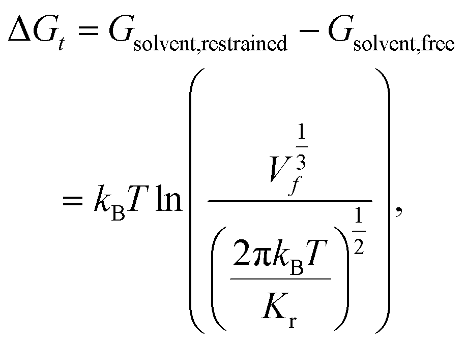 | (2) |
| ΔG = Gbilayer − Gsolvent,restrained + (Gsolvent,restrained − Gsolvent,free) = min(Gstage I) − min(Gstage III) + ΔGt. | (3) |
Evaluation of ΔG for a single ELP candidate requires a total of approximately 30 GPU h by running in parallel on 8× NVIDIA RTX 2080 Ti GPU cards.
2.3 Active learning optimization of ΔG
Having characterized the association free energy ΔG of single peptide chain into the vesicle bilayer, we want to minimize this ΔG (i.e., making it as negative as possible) with respect to the ELP sequence so as to maximize the stability of vesicle. This can be viewed as a black-box optimization problem of an unknown functional mapping y = f(x), where the target output is the association free energy y = ΔG(x) and the ELP sequence x is controlled by specifying the two guest residues and the lengths of the hydrophilic and hydrophobic blocks {X1,X2,m,n}. The unknown function can only be probed by running free energy calculations to compute ΔGi for a particular ELP sequence xi. Since the design space of (VPGX1G)m(VPGX2G)n ELPs is finite, we could in principle solve the optimization by brute force evaluation of ΔG for all candidate molecules. The high computational cost of the enhanced sampling free energy calculations makes this approach highly inefficient, and superior approaches rely on active learning (a.k.a., sequential learning, optimal experimental design) to perform principled identification of the most promising candidates to prioritize for computational screening.31,65–70 As we will show, after sampling sufficiently many candidates in the design space we can construct a surrogate model that is capable of accurately predicting the association free energy for unsampled candidates within the design space. We solve our optimization problem using a combination of Gaussian process regression (GPR) to construct data-driven surrogate models ŷ =![[f with combining circumflex]](https://www.rsc.org/images/entities/i_char_0066_0302.gif) (x) and Bayesian optimization (BO) to interrogate these models to identify the next most promising candidate to simulate.65 A schematic overview of the active learning pipeline is shown in Fig. 5.
(x) and Bayesian optimization (BO) to interrogate these models to identify the next most promising candidate to simulate.65 A schematic overview of the active learning pipeline is shown in Fig. 5.
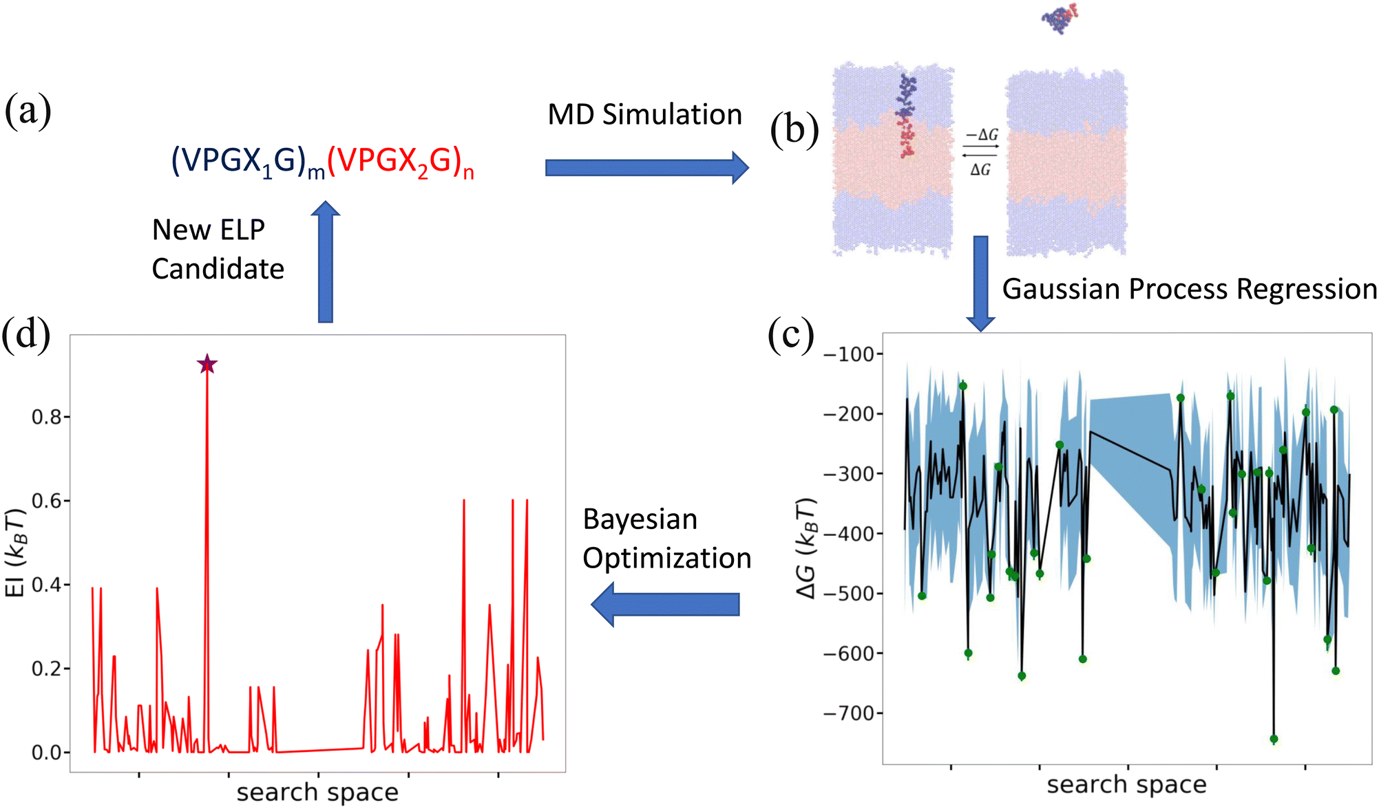 | ||
Fig. 5 Active learning cycle for data-driven identification of ELP sequences capable of assembling thermodynamically stable vesicles. (a) The ELP design space comprises the 168 diblock amphiphilic ELPs of the form (VPGX1G)m(VPGX2G)n, where X1 is one of twelve hydrophilic amino acid residues (except proline) {G, T, S, W, Y, H, E, Q, D, N, K, R}, X2 is one of seven hydrophobic residues {I, V, L, F, C, M, A}, m = 5, and n = {4, 5}. (b) Enhanced sampling free energy calculations are conducted to compute the association free energy yi = ΔGi of a candidate ELP sequence xi defined by the parameters {Xi1, Xi2, mi, ni}. (c) All ELP sequences simulated to date define the training data ![[scr D, script letter D]](https://www.rsc.org/images/entities/i_char_e523.gif) 1:t = {(x1,y1),…, (xt,yt)} over which we train a GPR model ŷ = (x) to predict the association free energies of ELP candidates outside the training set. The green dots represent the training points, the black line the GPR predicted mean, and the blue shading the GPR predicted standard deviation (i.e., uncertainty) in the mean prediction. For visual convenience, the GPR model ŷ = (x) is represented over a 1D projection into the highest variance direction within the sequence space calculated by multidimensional scaling59 based on the Jukes–Cantor distance between biological sequences.60 As such, the plot represents a projection of the multidimensional response surface and the topography of the surface should not be over-interpreted within this low-dimensional projection. (d) The GPR model is interrogated by a BO acquisition function known as the expected improvement EI(x) that prioritizes the unsampled ELP candidates within the design space most likely to possess high values of our objective function (i.e., minimize ΔG(x)). The red line indicates EI(x) within the 1D projection and we have indicated by a purple star the location of the top performing unsampled candidate (xt+1 = argmax EI(x)). The active learning cycle is closed by identifying this candidate xt+1 and subjecting it to the next round of enhanced sampling free energy calculations to compute yt+1, retrain the GPR model over the augmented training set 1:t+1 = 1:t+1 ∪ {(xt+1,yt+1)}, and perform a new round of BO to identify the next top performing ELP sequence. The iterative loop is terminated when the GPR model ceases to improve after multiple consecutive rounds indicating that we have fitted an accurate model over the full design space and/or we cease to see improvements in the top performing candidate identified in multiple consecutive rounds. 1:t = {(x1,y1),…, (xt,yt)} over which we train a GPR model ŷ = (x) to predict the association free energies of ELP candidates outside the training set. The green dots represent the training points, the black line the GPR predicted mean, and the blue shading the GPR predicted standard deviation (i.e., uncertainty) in the mean prediction. For visual convenience, the GPR model ŷ = (x) is represented over a 1D projection into the highest variance direction within the sequence space calculated by multidimensional scaling59 based on the Jukes–Cantor distance between biological sequences.60 As such, the plot represents a projection of the multidimensional response surface and the topography of the surface should not be over-interpreted within this low-dimensional projection. (d) The GPR model is interrogated by a BO acquisition function known as the expected improvement EI(x) that prioritizes the unsampled ELP candidates within the design space most likely to possess high values of our objective function (i.e., minimize ΔG(x)). The red line indicates EI(x) within the 1D projection and we have indicated by a purple star the location of the top performing unsampled candidate (xt+1 = argmax EI(x)). The active learning cycle is closed by identifying this candidate xt+1 and subjecting it to the next round of enhanced sampling free energy calculations to compute yt+1, retrain the GPR model over the augmented training set 1:t+1 = 1:t+1 ∪ {(xt+1,yt+1)}, and perform a new round of BO to identify the next top performing ELP sequence. The iterative loop is terminated when the GPR model ceases to improve after multiple consecutive rounds indicating that we have fitted an accurate model over the full design space and/or we cease to see improvements in the top performing candidate identified in multiple consecutive rounds. | ||
(x), which are most commonly parameterized using Gaussian process regression that naturally furnishes estimates of both the mean and uncertainties in the model predictions that are inputs to subsequent Bayesian optimal selection of the most promising next candidate for testing.65,71,72 The fundamental assumption of GPR modeling is that the target function f(x) is the realization of a Gaussian process over its inputs x with assumed zero mean and covariance function given by a kernel K that acts over pairs of inputs (a non-zero mean prior ν(x) can straightforwardly be incorporated by pretreating the data with the transformation y(x) ← y(x) − ν(x)72). That is, given a set of inputs X = {x1,…, xn}, the family of possible regression models fitting the data ![[f with combining right harpoon above (vector)]](https://www.rsc.org/images/entities/i_char_0066_20d1.gif) = {f(x1),f(x2),…, f(xn)} follow a multivariate Gaussian distribution ∼
= {f(x1),f(x2),…, f(xn)} follow a multivariate Gaussian distribution ∼ ![[scr N, script letter N]](https://www.rsc.org/images/entities/char_e52d.gif) (
(![[0 with combining right harpoon above (vector)]](https://www.rsc.org/images/entities/char_0030_20d1.gif) ,K(X,X)), where K(X,X) is the n × n Gram matrix whose components are K(xi,xj) (i.e., the value of the kernel function evaluated at data points xi and xj). Now, given a set of training data = {(x1,y1),…, (xn,yn)} where each yi = f(xi) + εi is a noisy observation of f(xi) and εi are assumed to be independent realizations of Gaussian noise following (0,σi2)), we obtain the joint distribution of
,K(X,X)), where K(X,X) is the n × n Gram matrix whose components are K(xi,xj) (i.e., the value of the kernel function evaluated at data points xi and xj). Now, given a set of training data = {(x1,y1),…, (xn,yn)} where each yi = f(xi) + εi is a noisy observation of f(xi) and εi are assumed to be independent realizations of Gaussian noise following (0,σi2)), we obtain the joint distribution of ![[y with combining right harpoon above (vector)]](https://www.rsc.org/images/entities/i_char_0079_20d1.gif) at the n training points and the target function values * at m testing points
at the n training points and the target function values * at m testing points  ,
,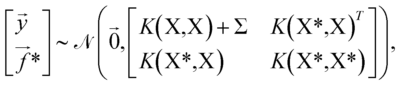 | (4) |
* given the training data is then,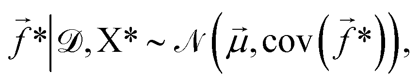 | (5) |
![[small mu, Greek, vector]](https://www.rsc.org/images/entities/i_char_e0e9.gif) and cov(*) are given by,
and cov(*) are given by,| = K(X*,X*)[K(X,X) + Σ]−1, | (6) |
| cov(*) = K(X*,X*) − K(X*,X)[K(X,X) + Σ]−1K(X*,X)T. | (7) |
![[small theta, Greek, vector]](https://www.rsc.org/images/entities/i_char_e1c8.gif) , and these parameters are optimized by maximizing the log-likelihood of training data,73
, and these parameters are optimized by maximizing the log-likelihood of training data,73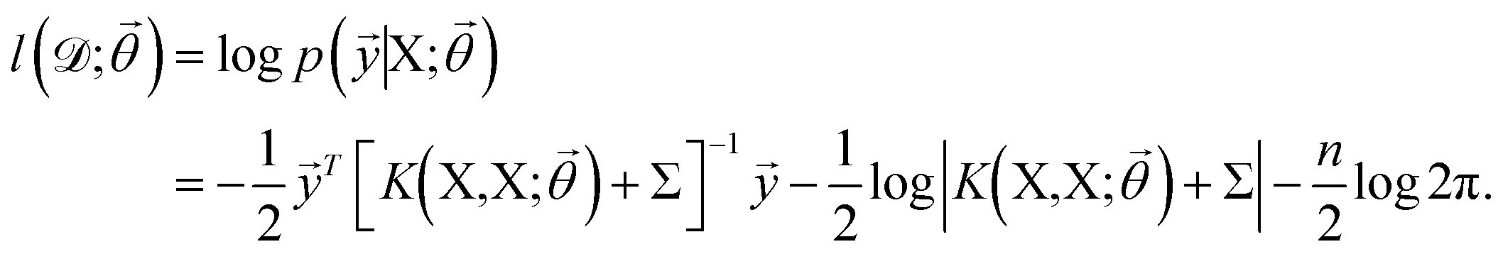 | (8) |
The key component in any GPR model is the choice of kernel function K.65,74 Valid kernels must be positive semi-definite to assure that for any set of inputs X = {x1,…, xn}, the Gram matrix K(X,X) is positive semi-definite.72 Moreover, in our case the inputs are amino acid strings, so we need kernels that operate on string data. Many string kernels have been proposed for peptide and protein data. For example, the Hamming distance kernel measures the number of positions containing the same amino acid residue within a pair of equal length strings, and the Levenshtein kernel is based on the minimal number of insertions, deletions, and replacements necessary to convert one string into another.75 The weighted degree kernel76 goes beyond single positions to compute similarity based on the co-occurrences of k-mers at corresponding positions within two equal length sequences. In our application, the size of the hydrophilic and hydrophobic blocks of the ELP can vary so it is vital that we employ a kernel capable of operating between strings of different lengths. In this work, we choose to adopt the generic string kernel of Giguère et al.,25 which defines the distance between two amino acid strings x = (x1,…, x|x|) and 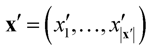 with, potentially unequal, lengths |x| and |x′| as,
 | (9) |
(xi) furnishes a prediction for the true performance yi = ΔGi of candidate ELP sequences xi that have not yet been simulated. Having fitted this model within a particular round of active learning, we now pass its predictions to a BO step that employs a so-called acquisition function u(x|) to define the relative prioritization of each unsampled candidate within the search space.65 Since we have a finitely enumerable design space and calculation of the acquisition function is computationally inexpensive, we can exhaustively compute the acquisition function for all candidates that have not yet been sampled. A number of choices of acquisition function are possible, but in this work we adopt the popular expected improvement (EI).65,78 Intuitively, this function ranks candidates according to their likelihood to outperform the current best candidate in the training data based on the predicted GPR mean and uncertainties. As such, this choice of acquisition function naturally optimizes under uncertainty, balances “exploit” (promoting candidates with large GPR predicted means) and “explore” (promoting candidates with large GPR predicted uncertainties) strategies, and can be used to perform principled interpolation and extrapolation within the design space. Mathematically, the EI for our minimization objective is defined as,65 | (10) |
(x) is the GPR prediction of y = ΔG following the posterior predictive distribution at x (eqn (5)) with mean μ(x) and standard deviation σ(x). is the training data comprising all simulated data points collected to date. f† = miny∈(y) is the minimum target function in the training data . Φ and ϕ are, respectively, the cumulative distribution function and probability density function of the standard normal distribution. ξ is a hyperparameter controlling the exploration-exploitation trade-off: higher values of ξ tend to favor regions in input space with high posterior uncertainty σ(x) while lower values of ξ tends to favor input space with lower posterior mean μ(x).65,79 We chose ξ = 0.01 as a standard choice.65 An intuitive way of interpreting eqn (10) is that it represents the expected degree of improvement relative to the current best minimum: max(f† − ξ − ,0) is equal to the reduction (f† − ξ − ) only if < (f† − ξ). The candidate with the greatest expected amount of reduction then becomes the next one to consider since we focus on minimizing the target function.
At each iteration of Bayesian optimization, we trained a GPR model based on the currently explored peptides 1:t. Then, for all the unexplored peptides, we compute the GPR posterior predictions of ΔG (eqn (5)) and evaluate the acquisition function (eqn (10)). Then we select one single peptide with the maximum acquisition function value as the next peptide to explore. Approaches exist to perform batched sampling of multiple simultaneous candidates in each BO round in order to maximize utilization of screening resources.80,81 In the present case, our enhanced sampling free energy calculations for each candidate are themselves embarrassingly parallel and so we maximize computational resource usage in sampling a single new candidate. We track round-to-round performance of the GPR/BO screening loop by monitoring the coefficient of determination R2 of GPR models during the fitting process by leave-one-out cross validation (LOO-CV), the Bhattacharyya distance between posterior Gaussian distributions (eqn (5)) returned by successive GPR models,82 and the objective function value f† = miny∈(y) of the best candidate discovered to date. When we observe convergence in all three of these metrics we can surmise that the GPR model has ceased to improve with additional data collection and the optimization may then be terminated.83 The terminal GPR is then applied globally to the candidate design space to predictively rank all candidates' performance. A summary of the GPR/BO iteration process is provided in Algorithm 1.
| Algorithm 1 Bayesian optimization |
|---|
| Initialize training data 0whileR2 or Bhattacharyya distance or f† do not plateau do Build GPR model based on Find xt = argmax u(x| Evaluate the (noisy) target function yt = f(xt) + εt Augment training data end while Output x* with minimum target function value in |
3 Results
3.1 Computational high-throughput screening of ELPs
We define our ELP design space as the 12 × 7 × 2 = 168 candidate diblock amphiphilic ELPs of the form (VPGX1G)5(VPGX2G)n, where X1 is one of twelve hydrophilic amino acid residues (except proline) categorized under the Kyte–Doolittle hydropathy scale23 {G, T, S, W, Y, H, E, Q, D, N, K, R}, X2 is one of seven hydrophobic residues {I, V, L, F, C, M, A}, and n = 4, 5. We choose n ≈ m since most experimental work on ELP vesicles tend to focus on nearly equally-sized hydrophilic and hydrophobic blocks.12,22 Experimentally, longer ELP chains are generally used. For example, Schreiber et al.12 have tested diblock ELPs with (n + m) = 70. Due to the longer equilibration times required for longer chains and the rapid increase in simulation box volume with chain length, we employ shorter chains with nearly equal number of hydrophilic and hydrophobic blocks to keep the ratio between hydrophilic and hydrophobic blocks similar to experiments, and hypothesize that the trends of ΔG that we see for shorter chains reflect the trends of ΔG for longer ones typically considered in experiments.The primary objective of this work is to discover amphiphilic diblock ELPs to maximize the thermodynamic stability of peptidic vesicles as novel chassis for synthetic cells. We assume that the vesicles are fabricated by a templated assembly mechanism such as solvent evaporation22,35 or emulsion transfer.14 Since we assume the vesicles are produced by directed assembly we need not program the molecules or environmental conditions to spontaneously self-assemble into a vesicle. Our only optimization criterion is to maximize the thermodynamic stability of peptides within the vesicle bilayer relative to an isolated peptide in bulk solvent. A deficiency of our approach is that we do not explicitly consider the relative thermodynamic stability of competing aggregates (e.g., micelles, sheets, gels). It is conceivable that alternative states not considered in our analysis may be more thermodynamically stable, but our motivating rationale is that placing the vesicle into a deep thermodynamic free energy well maximizes its lifetime by minimizing their propensity to disaggregate or transition into any alternative assembled structures due to both thermodynamic stabilization and kinetic trapping. As post hoc validation of this strategy, we find that one of the top performing (i.e., maximally thermodynamically stable) ELP sequences discovered by our screening is experimentally known and, even for such a short sequence, has been shown to form stable vesicles with lifetimes of several hours, with longer variants anticipated to form vesicles with lifetimes of months.12
We commenced our active learning screening by generating an initial set of 20 ELP sequences over the design space to serve as the initial training data for the GPR/BO models and pursued the active learning strategy described in section 2 interleaving successive rounds of enhanced sampling free energy calculations, Gaussian process regression, and Bayesian optimization (Fig. 5). We present in Table S1 in the ESI† an accounting of the full active learning screening showing the round in which each ELP candidate xi was sampled, its computed value of yi = ΔGi from enhanced sampling free energy calculations, and the predictions ŷi = (xi) of the terminal GPR model.
We present in Fig. 6 an illustrative PMF for one particular ELP sequence (VPGYG)5(VPGCG)4. In Fig. 6a we show our estimate of the 2D unbiased PMF G(zhead, ztail) computed by WHAM.56–58,61 For ease of visualization, in Fig. 6b we present a 1D projection G(zCOM) of the unbiased landscape into the center-of-mass displacement of the full ELP from the bilayer midplane.58 As expected, the value of PMF gradually rises when the chain is pulled from the bilayer out to the bulk solvent. Upon extension of the chain in bulk solvent, the PMF shows a weak relaxation as the chain is extended to its equilibrium length and then rises again as it is further extended. The ΔG value for this specific ELP sequence is calculated according to eqn (3), which, measured on a per amino acid residue basis, is ΔG = (−10.3 ± 0.4) kBT where uncertainties are estimated by five-fold block averaging. We note that the total free energy change is dominated by the first two stages of the umbrella sampling pathway (pulling the chain into the upper hydrophilic layer, extraction of the chain into bulk solvent), with the third stage (chain relaxation in bulk solvent) contributing less than 5% to the overall free energy for all ELP candidates considered within our screen. This suggests that the computational burden of the screen may be attenuated by omitting stage III of the umbrella sampling protocol without substantial loss of accuracy. Since the computational cost is dominated by the umbrella sampling calculations within the bilayer that require closely spaced umbrella windows, this would provide a modest computational savings of ∼4%.
 | ||
| Fig. 6 Illustrative PMF for (VPGYG)5(VPGCG)4. The hydrophilic (VPGYG)5 is shown in blue and the hydrophobic (VPGCG)4 block in red. The bilayer is made transparent to highlight the opaque pulled chain. Solvent and ions are not shown for clarity. (a) Two-dimensional unbiased PMF in the umbrella sampling collective variables G(zhead, ztail). (b) One-dimensional projection of the unbiased PMF G(zCOM) onto the center-of-mass displacement of the ELP from the bilayer midplane. The black, green and red dashed lines demarcate the three stages of the umbrella sampling pathway illustrated in Fig. 4. | ||
In Fig. 7 we illustrate our monitoring of the round-to-round performance of the GPR model over the course of the active learning screening by tracking the GPR coefficient of determination R2 under leave-one-out cross validation (LOO-CV), the Bhattacharyya distance between GPR posterior in successive rounds,82 and the cumulative minimum ΔG. We observe convergence of all three metrics after approximately six active learning rounds (i.e., after screening 20 + 6 = 26 ELP candidates) indicating that the trained GPR model is accurately predicting the performance of novel candidates, its posterior distribution has stabilized, and that we are no longer identifying new top performing candidates in our screen. These observations suggest that the 26 candidates over which we trained the GPR model are sufficiently representative in spanning the molecular design space that the model is not substantially changing upon the addition of more training points and that it can make quite accurate predictions over the remaining candidates within the space. We confirm that we have indeed reached convergence and the GPR model is no longer improving with successive training data by running our screening out to ten active learning rounds (i.e., 30 candidates, ∼18% of the 168-molecule design space) at which point we terminate the screen.
 | ||
| Fig. 7 Performance of the GPR models over the course of the active learning screening. (a) Coefficient of determination R2 measured by leave-one-out cross validation (LOO-CV). (b) Bhattacharyya distance between the posterior of successive GPR models in round i and (i + 1). (c) Top performing ELP candidate selected by maximizing the acquisition function in each particular round (points) and the cumulative top performer identified in any round so far (line). Error bars represent standard errors in ΔG estimated by five-fold block averaging. | ||
We present the top 10 ELP candidates identified by our active learning screening in Table 1. A full accounting of the ΔG values predicted by the terminal GPR model is provided in Table S1 in the ESI.† Our screening has identified a number of diverse ELP sequences capable of forming vesicle bilayers with large thermodynamic stabilities amounting to ΔG = 10–15kBT per amino acid residue. As illustrated in the table, we see no clear pattern in the hydrophobicity and hydrophilicity scores of the two guest residues in the top performing candidates. This appears to indicate the absence of simple single-residue design principles for amphiphilic diblock ELPs and that the active learning screening has uncovered more subtle multibody design rules for the engineering of vesicle thermostability. As an encouraging post hoc validation of our active learning screening and choice of objective function, our screening discovered as the fourth-ranked candidate the (VPGHG)5(VPGLG)4 sequence that has been experimentally demonstrated by Schreiber et al. to form stable vesicles with lifetime of several hours.12 The remaining sequences have not, to our knowledge, been previously experimentally investigated. Interestingly, our screening quite strongly favors histidine as the guest residue in the hydrophilic block although we see more diversity in the residue identity in the hydrophobic block. Possessing ΔG per residue values 0.2–1.5kBT lower than the experimentally demonstrated (VPGHG)5(VPGLG)4 sequence, we propose that these candidates may represent particularly interesting opportunities for future experimental testing and the assembly of ultrastable peptidic vesicles. For computational tractability this study has focused on relatively short 45–50 residue peptides, but we conjecture that the rank ordering of the measured thermostabilities will be preserved upon moving to the ∼350-residue peptides frequently employed in experiment.
| ELP sequence | Computed ΔG per residue (kBT) | Discovery iteration | Hydropathy score of X1 | Hydropathy score of X2 | Previously known? |
|---|---|---|---|---|---|
| H5V5 | −14.9 ± 0.2 | 2 | −3.2 | 4.2 | No |
| H5F4 | −14.2 ± 0.2 | 5 | −3.2 | 2.8 | No |
| H5V4 | −13.5 ± 0.1 | 3 | −3.2 | 4.2 | No |
| H5L4 | −13.3 ± 0.3 | 0 | −3.2 | 3.8 | Ref. 12 |
| H5F5 | −12.6 ± 0.1 | 6 | −3.2 | 2.8 | No |
| H5L5 | −11.5 ± 0.4 | 1 | −3.2 | 3.8 | No |
| H5C4 | −11.3 ± 0.1 | 4 | −3.2 | 2.5 | No |
| Y5F4 | −11.2 ± 0.1 | 0 | −1.3 | 2.8 | No |
| H5A4 | −10.5 ± 0.2 | 7 | −3.2 | 1.8 | No |
| Y5I4 | −10.4 ± 0.3 | 0 | −1.3 | 4.5 | No |
4 Discussions and conclusions
Elastin-like polypeptides are promising candidates that could serve an alternative chassis materials for synthetic cells that are more mechanically and chemically robust than constructs based on lipid membranes while maintaining biocompatibility.7,8,11,12,84 Peptidic vesicles formed by these building blocks could resemble the structure and functionality of living cells, thus making them suitable for a wide range of applications such as fundamental understanding of cellular activities85 or smart drug delivery.2 In this work, we report an active learning computational screen to discover diblock amphiphilic ELPs that could form stable peptidic vesicles. Our approach uses molecular simulation to obtain a quantitative measurement of the stability of the pre-assembled vesicle, and then employs Bayesian optimization to discover the promising diblock ELPs that maximize this stability. The optimization procedure converges after 10 iterations in which we computationally explore 30 ELP sequences corresponding to ∼18% of the 168-molecule design space at a cost of ∼900 GPU h of computation. Our screening identifies a number of high performing ELPs capable of forming highly stable vesicles and also identifies as our fourth-ranked candidate a previously known sequence that has been experimentally demonstrated to form vesicles with stabilities of multiple hours.12 Longer variants of these peptides with repeat lengths more in line with what is frequently explored in experiment are anticipated to be capable of forming vesicles with lifetimes of months.12 It is our immediate plan to subject the top ranked ELP sequences identified by this computational screen to experimental testing. We also propose to experimentally assay a number of predicted lower performing sequences as controls to test our use of ΔG as a computational measure of vesicle stability and experimentally validate the computational screening.In future work, we would expand the search space to longer chains. Experimentally, the diblock ELPs usually contain dozens of hydrophobic and hydrophilic blocks that enable relatively thick vesicles to be formed.11,12,21,22 These larger vesicles structurally resemble the compartments of biological cells1 and enable encapsulation of interesting bioactivities, such as compartmentalized peptide synthesis.11 Besides diblock ELPs, triblock ELPs with hydrophilic blocks on two ends and hydrophobic blocks in the middle have also been experimentally explored to form vesicles.32 Therefore, in future work it would be interesting to expand the search space to include larger diblock and triblock ELPs. It would also be interesting to consider other thermodynamic state points in temperature, pressure, and salt concentration to determine the degree to which the ELP rank ordering computed in this work is transferably preserved under other conditions relevant to the intended deployment environments for these vesicles. Although in principle the generic string kernel25 could operate on amino acid sequences with very different lengths, the evaluation of kernel could become computationally expensive as the sequence lengths grow.25 It might be helpful to first train an encoded representation, such as variational autoencoder66 or doc2vec model,86,87 to embed all peptides into an Euclidean space and perform Bayesian optimization over this embedding. The GPR model in this case would consist of kernel functions defined in the embedded space, such as radial basis kernel or Matérn kernel,73 that are less computationally expensive to evaluate. Another potential challenge is that the umbrella sampling simulations may become inefficient in larger systems due to the slower relaxation of the longer chains. Thus, it would be interesting to explore alternative enhanced sampling techniques, such as metadynamics52 or adaptive biasing force53 with the potential for improved sampling efficiencies. We also propose that our active learning screening approach can be generically extended to other applications in biopolymer and biomolecular design where it is necessary to navigate large sequence spaces by coupling the GPR/BO approach to alternative computational and/or experimental measures of performance such as protein–ligand binding free energy88 or antimicrobial activity.89,90
Author contributions
Y. M., A. P. L., and A. L. F. conceived the study. Y. M. and R. K. conducted the calculations. Y. M. and A. L. F. analyzed the data. Y. M. and A. L. F. wrote the paper. Y. M., B. S., A. P. L., and A. L. F. edited and critically revised the paper.Conflicts of interest
A. L. F. is a co-founder and consultant of Evozyne, Inc. and a co-author of US Patent Application 16/887710, US Provisional Patent Applications 62/853919, 62/900420, and 63/314898 and International Patent Applications PCT/US2020/035206 and PCT/US2020/050466.Acknowledgements
This work is supported by the National Science Foundation under Grant No. DMR-1939534 (A. P. L.) and DMR-1939463 (A. L. F.). This work was completed in part with resources provided by the University of Chicago Research Computing Center. We gratefully acknowledge computing time on the University of Chicago high-performance GPU-based cyberinfrastructure supported by the National Science Foundation under Grant No. DMR-1828629.Notes and references
- P. Stano, Life, 2018, 9, 3 CrossRef.
- Y. Elani, R. V. Law and O. Ces, Ther. Delivery, 2015, 6, 541–543 CrossRef CAS PubMed.
- C. Xu, S. Hu and X. Chen, Mater. Today, 2016, 19, 516–532 CrossRef CAS PubMed.
- I. Ivanov, S. L. Castellanos, S. Balasbas, L. Otrin, N. Marušič, T. Vidaković-Koch and K. Sundmacher, Annu. Rev. Chem. Biomol. Eng., 2021, 12, 287–308 CrossRef CAS.
- V. Noireaux and A. P. Liu, Annu. Rev. Biomed. Eng., 2020, 22, 51–77 CrossRef CAS PubMed.
- K. A. Podolsky and N. K. Devaraj, Nat. Rev. Chem., 2021, 5, 676–694 CrossRef CAS.
- L. Sercombe, T. Veerati, F. Moheimani, S. Y. Wu, A. K. Sood and S. Hua, Front. Pharmacol., 2015, 6, 286 Search PubMed.
- J. A. Jackman, J. H. Choi, V. P. Zhdanov and N. J. Cho, Langmuir, 2013, 29, 11375–11384 CrossRef CAS PubMed.
- B. M. Discher, Y.-Y. Won, D. S. Ege, J. C. M. Lee, F. S. Bates, D. E. Discher and D. A. Hammer, Science, 1999, 284, 1143–1146 CrossRef CAS.
- A. Groaz, H. Moghimianavval, F. Tavella, T. W. Giessen, A. G. Vecchiarelli, Q. Yang and A. P. Liu, Wiley Interdiscip. Rev.: Nanomed. Nanobiotechnol., 2021, 13, e1685 CAS.
- K. Vogele, T. Frank, L. Gasser, M. A. Goetzfried, M. W. Hackl, S. A. Sieber, F. C. Simmel and T. Pirzer, Nat. Commun., 2018, 9, 1–7 CrossRef CAS.
- A. Schreiber, M. C. Huber and S. M. Schiller, Langmuir, 2019, 35, 9593–9610 CrossRef CAS PubMed.
- M. K. Pastuszka, X. Wang, L. L. Lock, S. M. Janib, H. Cui, L. D. DeLeve and J. A. MacKay, J. Controlled Release, 2014, 191, 15–23 CrossRef CAS PubMed.
- B. Sharma, Y. Ma, H. L. Hiraki, B. M. Baker, A. L. Ferguson and A. P. Liu, Chem. Commun., 2021, 57, 13202–13205 RSC.
- D. H. T. T. Le and A. Sugawara-Narutaki, Mol. Syst. Des. Eng., 2019, 4, 545–565 RSC.
- S. Roberts, M. Dzuricky and A. Chilkoti, FEBS Lett., 2015, 589, 2477–2486 CrossRef CAS PubMed.
- A. Yeboah, R. I. Cohen, C. Rabolli, M. L. Yarmush and F. Berthiaume, Biotechnol. Bioeng., 2016, 113, 1617–1627 CrossRef CAS PubMed.
- D. W. Urry, Prog. Biophys. Mol. Biol., 1992, 57, 23–57 CrossRef CAS.
- M. H. Misbah, L. Quintanilla, M. Alonso and J. C. Rodríguez-Cabello, Polymer, 2015, 81, 37–44 CrossRef CAS.
- D. Juanes-Gusano, M. Santos, V. Reboto, M. Alonso and J. C. Rodríguez-Cabello, J. Pept. Sci., 2022, 28, e3362 CrossRef CAS.
- A. Schreiber, L. G. Stühn, M. C. Huber, S. E. Geissinger, A. Rao and S. M. Schiller, Small, 2019, 15, 1900163 CrossRef PubMed.
- T. Frank, K. Vogele, A. Dupin, F. C. Simmel and T. Pirzer, Chem. – Eur. J., 2020, 26, 17356–17360 CrossRef CAS.
- J. Kyte and R. F. Doolittle, J. Mol. Biol., 1982, 157, 105–132 CrossRef CAS PubMed.
- P. Zhou, X. Chen, Y. Wu and Z. Shang, Amino Acids, 2010, 38, 199–212 CrossRef CAS.
- S. Giguère, M. Marchand, F. Laviolette, A. Drouin and J. Corbeil, BMC Bioinf., 2013, 14, 1–16 CrossRef.
- E. Y. Lee, G. C. L. Wong and A. L. Ferguson, Bioorg. Med. Chem., 2018, 26, 2708–2718 CrossRef CAS.
- M. Nielsen and O. Lund, BMC Bioinf., 2009, 10, 296 CrossRef.
- C. S. Leslie, E. Eskin, A. Cohen, J. Weston and W. S. Noble, Bioinformatics, 2004, 20, 467–476 CrossRef CAS PubMed.
- E. Y. Lee, B. M. Fulan, G. C. L. Wong and A. L. Ferguson, Proc. Natl. Acad. Sci. U. S. A., 2016, 113, 13588–13593 CrossRef CAS PubMed.
- Y. Lei, S. Li, Z. Liu, F. Wan, T. Tian, S. Li, D. Zhao and J. Zeng, Nat. Commun., 2021, 12, 5465 CrossRef CAS.
- B. Mohr, K. Shmilovich, I. S. Kleinwächter, D. Schneider, A. L. Ferguson and T. Bereau, Chem. Sci., 2022, 13, 4498–4511 RSC.
- L. Martín, E. Castro, A. Ribeiro, M. Alonso and J. C. Rodríguez-Cabello, Biomacromolecules, 2012, 13, 293–298 CrossRef PubMed.
- T. Luo, M. A. David, L. C. Dunshee, R. A. Scott, M. A. Urello, C. Price and K. L. Kiick, Biomacromolecules, 2017, 18, 2539–2551 CrossRef CAS PubMed.
- A. Prhashanna, P. A. Taylor, J. Qin, K. L. Kiick and A. Jayaraman, Biomacromolecules, 2019, 20, 1178–1189 CrossRef CAS.
- H. R. Marsden, L. Gabrielli and A. Kros, Polym. Chem., 2010, 1, 1512–1518 RSC.
- Schrödinger LLC, The PyMOL Molecular Graphics System (Version 2.0).
- D. H. De Jong, G. Singh, W. F. Bennett, C. Arnarez, T. A. Wassenaar, L. V. Schäfer, X. Periole, D. P. Tieleman and S. J. Marrink, J. Chem. Theory Comput., 2013, 9, 687–697 CrossRef CAS PubMed.
- S. J. Marrink and D. P. Tieleman, Chem. Soc. Rev., 2013, 42, 6801–6822 RSC.
- L. Darré, M. R. Machado, A. F. Brandner, H. C. González, S. Ferreira and S. Pantano, J. Chem. Theory Comput., 2015, 11, 723–739 CrossRef.
- M. R. Machado, E. E. Barrera, F. Klein, M. Sóñora, S. Silva and S. Pantano, J. Chem. Theory Comput., 2019, 15, 2719–2733 CrossRef CAS PubMed.
- L. Monticelli, S. K. Kandasamy, X. Periole, R. G. Larson, D. P. Tieleman and S.-J. Marrink, J. Chem. Theory Comput., 2008, 4, 819–834 CrossRef CAS PubMed.
- J. E. Condon, T. B. Martin and A. Jayaraman, Soft Matter, 2017, 13, 2907–2918 RSC.
- G. Bussi, D. Donadio and M. Parrinello, J. Chem. Phys., 2007, 126, 14101 CrossRef PubMed.
- H. J. C. Berendsen, J. P. M. Postma, W. F. Van Gunsteren, A. Dinola and J. R. Haak, J. Chem. Phys., 1984, 81, 3684–3690 CrossRef CAS.
- M. Parrinello and A. Rahman, Phys. Rev. Lett., 1980, 45, 1196–1199 CrossRef CAS.
- R. W. Hockney and J. W. Eastwood, Computer Simulation Using Particles, crc Press, 2021 Search PubMed.
- M. J. Abraham, T. Murtola, R. Schulz, S. Páll, J. C. Smith, B. Hess and E. Lindah, SoftwareX, 2015, 1–2, 19–25 CrossRef.
- W. Humphrey, A. Dalke and K. Schulten, J. Mol. Graphics, 1996, 14, 33–38 CrossRef CAS PubMed.
- J. A. Lemkul and D. R. Bevan, J. Phys. Chem. B, 2010, 114, 1652–1660 CrossRef CAS.
- E. Sevgen, M. Dolejsi, P. F. Nealey, J. A. Hubbell and J. J. De Pablo, Macromolecules, 2018, 51, 9538–9546 CrossRef CAS.
- R. C. Bernardi, M. C. R. Melo and K. Schulten, Biochim. Biophys. Acta, Gen. Subj., 2015, 1850, 872–877 CrossRef CAS.
- A. Barducci, M. Bonomi and M. Parrinello, Wiley Interdiscip. Rev.: Comput. Mol. Sci., 2011, 1, 826–843 CAS.
- J. Comer, J. C. Gumbart, J. Hénin, T. Lelièvre, A. Pohorille and C. Chipot, J. Phys. Chem. B, 2015, 119, 1129–1151 CrossRef CAS PubMed.
- G. M. Torrie and J. P. Valleau, J. Comput. Phys., 1977, 23, 187–199 CrossRef.
- M. R. Shirts and J. D. Chodera, J. Chem. Phys., 2008, 129, 124105 CrossRef PubMed.
- S. Kumar, J. M. Rosenberg, D. Bouzida, R. H. Swendsen and P. A. Kollman, J. Comput. Chem., 1992, 13, 1011–1021 CrossRef CAS.
- B. Roux, Comput. Phys. Commun., 1995, 91, 275–282 CrossRef CAS.
- A. L. Ferguson, J. Comput. Chem., 2017, 38, 1583–1605 CrossRef CAS.
- M. C. Hout, M. H. Papesh and S. D. Goldinger, Wiley Interdiscip. Rev. Cogn. Sci., 2013, 4, 93–103 CrossRef PubMed.
- S. Jeffery, Biochem. Soc. Trans., 1979, 7, 452–453 CrossRef.
- A. Grossfield, WHAM: The weighted histogram analysis method, https://membrane.urmc.rochester.edu/wordpress/?page_id=126 Search PubMed.
- J. Hermans and L. Wang, J. Am. Chem. Soc., 1997, 119, 2707–2714 CrossRef CAS.
- B. Lai and C. Oostenbrink, Theor. Chem. Acc., 2012, 131, 1–13 Search PubMed.
- M. Zhao, K. J. Lachowski, S. Zhang, S. Alamdari, J. Sampath, P. Mu, C. J. Mundy, J. Pfaendtner, J. J. De Yoreo, C.-L. Chen and others, Biomacromolecules, 2022, 23, 992–1008 CrossRef CAS PubMed.
- B. Shahriari, K. Swersky, Z. Wang, R. P. Adams and N. De Freitas, Proc. IEEE, 2016, 104, 148–175 Search PubMed.
- K. Shmilovich, R. A. Mansbach, H. Sidky, O. E. Dunne, S. S. Panda, J. D. Tovar and A. L. Ferguson, J. Phys. Chem. B, 2020, 124, 3873–3891 CrossRef CAS PubMed.
- K. Shmilovich, S. S. Panda, A. Stouffer, J. D. Tovar and A. L. Ferguson, Digital Discovery, 2022, 1, 448–462 RSC.
- C. Kim, A. Chandrasekaran, A. Jha and R. Ramprasad, MRS Commun., 2019, 9, 860–866 CrossRef CAS.
- J. Ling, M. Hutchinson, E. Antono, S. Paradiso and B. Meredig, Integr. Mater. Manuf. Innov., 2017, 6, 207–217 CrossRef.
- R. Gómez-Bombarelli, J. N. Wei, D. Duvenaud, J. M. Hernández-Lobato, B. Sánchez-Lengeling, D. Sheberla, J. Aguilera-Iparraguirre, T. D. Hirzel, R. P. Adams and A. Aspuru-Guzik, ACS Cent. Sci., 2018, 4, 268–276 CrossRef.
- C. E. Rasmussen, Advanced Lectures on Machine Learning: ML Summer Schools 2003, Canberra, Australia, February 2 - 14, 2003, Tübingen, Germany, August 4 - 16, 2003, Revised Lectures, Springer Berlin Heidelberg, Berlin, Heidelberg, 2004, pp. 63–71 Search PubMed.
- C. K. Williams and C. E. Rasmussen, Gaussian Processes for Machine Learning, MIT press, Cambridge, MA, 2006, vol. 2 Search PubMed.
- E. Schulz, M. Speekenbrink and A. Krause, J. Math. Psychol., 2018, 85, 1–16 CrossRef.
- D. Duvenaud, PhD thesis, University of Cambridge, 2014, DOI:10.17863/CAM.14087.
- J. Xu and X. Zhang, IEEE International Conference on Neural Networks - Conference Proceedings, 2004, vol. 4, pp. 3015–3018 Search PubMed.
- S. Sonnenburg, G. Rätsch, C. Schäfer and B. Schölkopf, J. Mach. Learn. Res., 2006, 7, 1531–1565 Search PubMed.
- S. Henikoff and J. G. Henikoff, Proc. Natl. Acad. Sci. U. S. A., 1992, 89, 10915–10919 CrossRef CAS PubMed.
- J. Mockus, V. Tiesis and A. Zilinskas, Towards Global Optimisation, 1978, vol. 2, pp. 117–129 Search PubMed.
- K. Wang and A. W. Dowling, Curr. Opin. Chem. Eng., 2022, 36, 100728 CrossRef.
- D. Ginsbourger, R. Le Riche and L. Carraro, A Multi-points Criterion for Deterministic Parallel Global Optimization based on Gaussian Processes, hal-00260579 Technical Report, https://hal.archives-ouvertes.fr/hal-00260579, 2008 Search PubMed.
- J. Wang, S. C. Clark, E. Liu and P. I. Frazier, Oper. Res., 2020, 68, 1850–1865 CrossRef.
- A. Bhattacharyya, Sankhya, 1946, 7, 401–406 Search PubMed.
- G. Beatty, E. Kochis and M. Bloodgood, 2019 IEEE 13th International Conference on Semantic Computing (ICSC), 2019, pp. 287–294 Search PubMed.
- B. Sharma, Y. Ma, A. L. Ferguson and A. P. Liu, Soft Matter, 2020, 16, 10769–10780 RSC.
- W. Sato, T. Zajkowski, F. Moser and K. P. Adamala, Wiley Interdiscip. Rev.: Nanomed. Nanobiotechnol., 2022, 14, e1761 CAS.
- K. K. Yang, Z. Wu, C. N. Bedbrook and F. H. Arnold, Bioinformatics, 2018, 34, 2642–2648 CrossRef CAS.
- Q. Le and T. Mikolov, Proceedings of the 31st International Conference on Machine Learning, Bejing, China, 2014, pp. 1188–1196 Search PubMed.
- H.-J. Woo and B. Roux, Proc. Natl. Acad. Sci. U. S. A., 2005, 102, 6825–6830 CrossRef CAS.
- C. Chen, F. Pan, S. Zhang, J. Hu, M. Cao, J. Wang, H. Xu, X. Zhao and J. R. Lu, Biomacromolecules, 2010, 11, 402–411 CrossRef CAS.
- Z. Ma, X. Liu, J. Nie, H. Zhao and W. Li, Biomacromolecules, 2022, 23, 1302–1313 CrossRef CAS.
Footnotes |
| † Electronic supplementary information (ESI) available: Table S1 listing the round in which each ELP candidate xi was sampled within the active learning screen, computed values of yi = ΔGi from enhanced sampling free energy calculations, and predictions ŷi = (xi) of the terminal GPR model. See DOI: https://doi.org/10.1039/d2me00169a |
| ‡ Present address: Department of Chemistry and Chemical Biology, Rutgers University-New Brunswick, Piscataway, New Jersey 08854, USA. |
| This journal is © The Royal Society of Chemistry 2023 |