
 Open Access Article
 This Open Access Article is licensed under a Creative Commons Attribution-Non Commercial 3.0 Unported Licence
Theoretical and computational methodologies for understanding coordination self-assembly complexes
Satoshi
Takahashi
 *a,
Satoru
Iuchi
b,
Shuichi
Hiraoka
a and
Hirofumi
Sato
*cd
*a,
Satoru
Iuchi
b,
Shuichi
Hiraoka
a and
Hirofumi
Sato
*cd
aDepartment of Basic Science, Graduate School of Arts and Sciences, The University of Tokyo, 3-8-1 Komaba, Meguro-ku, Tokyo 153-8902, Japan. E-mail: ghnr5571@g.ecc.u-tokyo.ac.jp
bGraduate School of Informatics, Nagoya University, Furo-cho, Chikusa-ku, Nagoya 464-8601, Japan
cDepartment of Molecular Engineering, Kyoto University, Nishikyo-ku, Kyoto 615-8510, Japan. E-mail: hirofumi@moleng.kyoto-u.ac.jp
dFukui Institute for Fundamental Chemistry, Kyoto University, Sakyo-ku, Kyoto 606-8103, Japan
First published on 13th April 2023
Abstract
This perspective highlights three theoretical and computational methods to capture the coordination self-assembly processes at the molecular level: quantum chemical modeling, molecular dynamics, and reaction network analysis. These methods cover the different scales from the metal–ligand bond to a more global aspect, and approaches that are best suited to understand the coordination self-assembly from different perspectives are introduced. Theoretical and numerical researches based on these methods are not merely ways of interpreting the experimental studies but complementary to them.
1 Introduction
Molecular self-assembly is a chemical process in which constituent units become spontaneously arranged structures based on intermolecular interactions.1–4 It is one of the most fundamental strategies for imparting function to materials in biological and artificial systems. From the nanoscale to the macroscale, many structures that support life are built by molecular self-assembly. In other words, life has been constructed by highly complex chemical systems based on the fundamental principle of molecular self-assembly, which has evolved over many years. Understanding the fundamental rule governing artificial systems is also vital in applying molecular self-assembly to materials science which has also made significant progress over the past several decades. Here in this article, we report theoretical and numerical methodologies on the discrete coordination self-assembly complexes, which consists of organic multitopic ligands (L) and metal ions (M), with the contributions of the present authors being highlighted. One of the reasons why the coordination self-assembly is focused on is that bonding patterns between the building blocks and the resultant structures of the products are well-defined compared to other artificial or biological self-assembly systems due to the coordination number and direction of the metal being strictly fixed. We believe that the insights obtained through the studies introduced in this paper are available in other molecular self-assembly systems.As a matter of course, the research of molecular self-assembly had been led by experimental studies. However, as the interests and concerns are getting directed not only to the final products but also to the global reaction process, the situations and approaches should change in order to track the reaction pathways and obtain the information about dominant elementary reactions, rate-determining steps, kinetic traps, etc. Even with the state-of-the-art experimental techniques, it is very difficult (practically impossible) to observe all the intermediate species transiently produced in the course of the self-assembly. The past experimental studies explicitly associated with the reaction process were limited to the self-assembly systems in which long-lived intermediate species could be experimentally observed. However, as will be exemplified later, it is not clear whether these long-lived species are really on the main reaction pathway or not, because those species too rapidly converting to the next intermediates cannot be observed experimentally even if those are on the main pathway. Additionally, it is not possible to determine with experiments alone what kind of microscopic behavior is occurring at the level of electronic states in leading to the final assembly product. Therefore, it is natural that a different approach, which is not only a mere follow-up tool but also hopefully supportive, should be taken to obtain more reaction details, with theoretical/computational tools appearing as the most suitable candidates. Another advantage arising from experimental research going hand in hand with theoretical research is that the laborious and costly experimental manipulations, material and experimental designs that must be performed to reach the desired results can be minimized with the help of theoretical predictions.
From theoretical and computational points of view, the well-arranged, final geometrical structure is thought to be determined as the free energy minima of the system's potential (or free) energy hypersurface. Hence, two aspects are critical to the understanding of the process. One is how to evaluate the surface, and the other is how the system develops on the surface. Namely, these two may be considered to focus on local and global aspects of the surface. For the former, accurate computation of the formation energy is a primary concern. In particular, bond formation between M–L is the key because the interaction requires the quantum chemical description. Although multi-configuration ab initio theory such as CASSCF might be needed to adequately describe the electronic structure of coordination self-assembly complexes, widely used density functional theory (DFT) could be a more reasonable choice because of its handiness and computational costs. However, it should be pointed out that because many isomers and intermediates exist in an assembly process, more rapid computations are necessary to sufficiently explore a wide area of the surface to grasp the landscape of the energy surface.5,6 Using classical-type potential, such as molecular mechanics (MM), is sufficiently cheap in computations but the treatment of M–L bond is usually infeasible due to the lack of quantum mechanical description, especially a proper consideration of d-electrons.7 For the latter, the idea of reaction pathways embedded in a complex reaction network is inevitably related to the concept of the energy landscape. That is, expected chemical species or microstates like conformers are located at the local minima of the energy landscape and reactions indicating the events of overcoming transition states are connecting those local minima. In this view, a well-defined kinetically controlled reaction pathway can be created by suitably modulating the corresponding energy landscape in some manners. There are some pioneering previous studies, for example, treating self-assembly pathways from the point of view of the energy landscape8 or showing the dynamical simulations of such processes.9 Putting the energy landscapes perspective in the context of the present article, products obtained through efficient molecular self-assembly requires the global energy landscape to have a single funnel, giving a well-defined minimum value of the free energy.10–12 Many such processes proceeding under thermodynamic control are interested in the yield of final products, and understanding the details of reaction pathways are considered to have nothing to do with both the preparation and the result of experiments. But in reality, the knowledge of reaction pathway details largely helps to rationally control the yield of the products under the kinetic control by modulating the energy landscape.
The present article is organized as follows. In the next section, we show some quantum chemical approaches for the coordination self-assembly, to abstract the reaction mechanism via the most fundamental level in molecular theory, that is, the electronic structure. In Section 3, researches that adopted the molecular dynamics (MD) simulations as the way to directly track the global process of the self-assembly are introduced. As another way for tracking the global process of the self-assembly from a panoramic point of view, Section 4 introduces kinetic studies based on the stochastic algorithm. Finally, we conclude this paper with an outlook.
2 Quantum chemical approach
To reveal structural details of coordination self-assembly systems, the directional coordination bonds, which are the key to the metal-complex formation, have to be described appropriately at the atomic level. The directionality of M–L bonds originates from the effects of metal d-electrons and thus incorporating the d-electron effects is the key to computational methods. In this section, various computational methods are briefly outlined in terms of the description of the directional coordination bonds. Then, quantum mechanical modelings to include the d-electron effects are focused with emphasis on their concepts. Finally, applications of the aforementioned computational methods are outlined in terms of computations on structural characteristics of metal-containing systems. Note that various computational methods are comprehensively reviewed for metallo-organic cages with broader perspectives in other literatures.5,62.1 Brief overview of various computational approaches
In terms of computational costs, MM is one of the most attractive approaches to explore large molecular structures including self-assembly systems. However, the MM force fields are not based on quantum mechanical description and do not include the d-electron effects explicitly. By contrast, ab initio electronic structure and DFT methods naturally describe the directional coordination bonds by construction. In particular, the wavefunction-based ab initio approaches such as the multireference perturbation methods include the electron correlation effects, which are important for metal containing systems, with high accuracy. However, the computational costs become problematic for large metal containing systems. On the other hand, DFT calculations provide reasonably accurate results with less computational costs for metal containing systems. In this respect, the first-principle DFT calculation is an approach suitable for computations of large metal containing systems including coordination self-assembly. The tight-binding DFT method, which is a semiempirical method, has also attracted interest in applications to metal-containing systems.13,14Several quantum mechanical approaches have been also developed to include the d-electron effects. The electronic structures of transition metal complexes have been often interpreted by the crystal field (CF) or ligand field (LF) theories, where the electronic d–d states arising from the (nd)Nd configurations with Nd being the number of d-electrons are described by the CF or LF contributions and the repulsions between the d-electrons.15 In the CF or LF pictures, the metal d-orbitals are split in energy due to the field on the metal ion created by surrounding ligands. An approach to incorporate such LF contributions (the d-orbital splittings) into force fields has been developed.7 On the other hand, an effective model Hamiltonian approach has been developed to incorporate both the M–L interactions and the d-electron repulsions explicitly, with having wavefunctions in a d-orbital space.16,17 A more rigorous effective Hamiltonian approach named the effective Hamiltonian crystal field (EHCF) method18,19 has been developed to describe d–d states of transition metal containing systems. In the next section, these quantum mechanical approaches for metal containing systems are focused with emphasis on their concepts.
2.2 Quantum mechanical methods to incorporate d-electron effects
In the LF picture, the d orbital energies can be computed by the diagonalization of the 5 × 5 ligand field matrix VLF, composing of the one-electron matrix elements, 〈di|![[v with combining circumflex]](https://www.rsc.org/images/entities/i_char_0076_0302.gif) LF|dj〉.15 In the CF picture, surrounding ligands are simply modeled by charges and LF is described only by the electrostatic contribution. However, the M–L bonds include covalent character to some extent, and the interactions between the metal d and ligand orbitals should be considered. The angular overlap model (AOM) describes the d-orbital splittings by parametrizing the M–L orbital interactions of M–L bond.15,20 Because the orbital interactions are connected with the overlap integrals between the metal d and ligand orbitals, the total LF effects are given as a sum of the individual M–L bond contributions as7
LF|dj〉.15 In the CF picture, surrounding ligands are simply modeled by charges and LF is described only by the electrostatic contribution. However, the M–L bonds include covalent character to some extent, and the interactions between the metal d and ligand orbitals should be considered. The angular overlap model (AOM) describes the d-orbital splittings by parametrizing the M–L orbital interactions of M–L bond.15,20 Because the orbital interactions are connected with the overlap integrals between the metal d and ligand orbitals, the total LF effects are given as a sum of the individual M–L bond contributions as7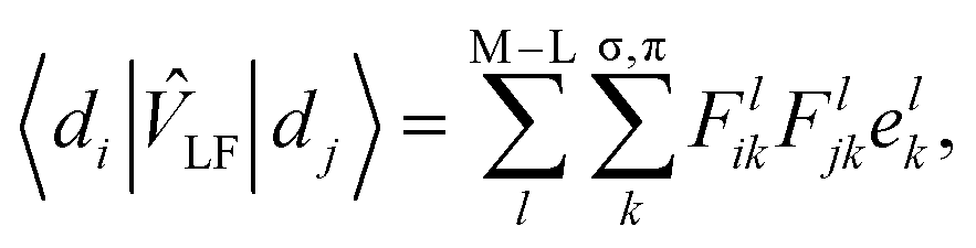 | (1) |
On the other hand, the Hamiltonian matrix including both the LF contributions and the d-electron repulsions on the basis of (nd)Nd configurations could automatically include the information on multiple electronic states. As such an approach, we have been developing a model effective Hamiltonian which can describe the d–d states of the central metal ion under the influence of surrounding ligands.16,17 In this approach, the electronic energy Em and the wavefunction Ψm for the mth d–d state at a given nuclear configuration R are computed by diagonalizing the model Hamiltonian matrix as
| Hmodel(R)Cm(R) = Em(R)Cm(R) | (2) |
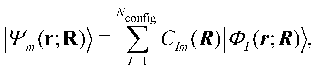 | (3) |
The key of the above model Hamiltonian is the proper modeling of the Hmodel matrix elements. Because only the metal d–d states are concerned, the (nd)Nd configurations with the ground state configuration of the ligands are primarily considered (P space). The ligand-to-metal charge-transferred configurations are considered as the other space (Q space). By this space division, an effective Hamiltonian Heff for the P space under the influence of the Q space is derived. Then, appropriate forms of the Hmodel matrix elements are determined through chemically intuitive arguments with the aid of Heff. By considering the nature of the P and Q spaces, the M–L electrostatic (ES) and exchange (EX) interactions are derived from the term only containing P space and the M–L charge transfer (CT) interaction is derived from the term containing the Q space. Therefore, the matrix elements are modeled as the sum of various M–L interaction related parts:
| (Hmodel)IJ = HMIJ + HESIJ + HEXIJ + HCTIJ. | (4) |
|dj〉, where is the electrostatic potential by the ligand charges. Similar to AOM, the EX and CT matrix elements are modeled by the appropriate overlap integrals between the d and ligand model orbitals. Several adjustable parameters employed in these matrix elements are determined so that the model Hamiltonian reasonably reproduces reference ab initio electronic structure and/or DFT calculation results. For example, the MCQDPT and DFT methods were chosen to obtain reference calculation results in ref. 16 and 17, respectively. Therefore, the model Hamiltonian could be an alternative of ab initio electronic structure and/or DFT calculations.
In the above model Hamiltonian approach, the effective Hamiltonian is derived in a simplified fashion for the use in modeling the Hamiltonian matrix elements. In the EHCF method,18,19,21,22 an effective Hamiltonian for transition metal containing systems is derived in a more rigorous fashion. In the ab initio electronic structure calculations, the electron correlation effects can be described by taking account of all the electronic configurations including metal and ligands. However, such full configuration interaction (CI) approach is infeasible in practice due to the computational costs. In the EHCF method, by dividing the valence orbitals of transition metal and ligand atoms into the d and l subsystems, the Hamiltonians for two subsystems are derived. As a result, a hybrid approach is realized in which only the d subsystem is deal with the (nd)Nd configurations. In this way, the d–d states are computed by the effective Hamiltonian of the d subsystem incorporating the effects from the l subsystem.
2.3 Applications of various approaches
In this subsection, applications of the aforementioned approaches are outlined in the same order as in Section 2.1. Note that applications to metal-containing systems other than the self-assembly ones are also included here.One of the drawbacks of force fields is the lack of transferability to arbitrary molecular systems because they are not based on quantum mechanical description. In fact, various force fields have been developed for limited class of systems, and there are various efforts to construct force fields specialized for metal containing systems.23 For example, in the cationic dummy atom (CaDA) model, the M–L electrostatic interactions are described by using the dummy charges placed around a metal ion to express the directionality of the M–L bonds. Several applications of this model to self-assembly systems are described in Section 3. On the other hand, a generic force field named GFN-FF24 has been developed to achieve fast structure optimizations for various chemical systems. It was shown that the GFN-FF optimized structures of metal–organic porous materials such as Pd46L96(BF4)96 agrees with the experimental crystal structures.24
As for the electronic structure theory calculations, the DFT calculations have been widely utilized for coordination self-assembly systems by considering the accuracy and computational costs. Efforts to improve DFT methods have been continuing for more accurate description of structural properties of large molecular systems, difficult to be explored by the wavefunction based ab initio methods such as CASSCF/CASPT2. The B97-3c composite method25 is an example, which has been tested for small molecule binding in metal–organic frameworks (MOFs) and porous organic cages.26 However, even the DFT methods have limitations on the system size due to their computational costs. Accurate tight binding DFTs, called GFNn-xTB, have been developed for the calculation of structures of large molecular systems13,14 and the applications include the structure optimization of the self-assembled [Pd12L24]24+.13 The GFNn-xTB method with the GBSA implicit solvation model has also applied to the structure optimizations of large metal complexes including self-assembly systems such as Pd30L60(BF4)60.27
The structures of transition metal complexes are often affected by electronic effects arising from various (nd)Nd electronic configurations, which are irrelevant to organic systems. The LFMM method is based on a quantum mechanical modeling and has successfully described these structural characteristics.7 For example, the LFMM method generated distorted structures of various Cu(II)N6 complexes which agree with experimental data.28 The structures could be different when the spin multiplicities are different, which has been also modeled by the LFMM.29,30 The LFMM method was also applied to simulating the CO2-induced flexibility of a flexible MOF31 and spin-crossover behavior in a MOF.32 In the LF theory, the LF effects and the d-electron repulsions have been regarded as parameters, extracted from experimental data on d–d spectra. In the LFMM case, the LF stabilizations are determined by the AOM parameters as shown in eqn (1). On the other hand, the quantum chemical methods to extract the LF related parameters have been proposed based on DFT33 and CASSCF and NEVPT2 calculations.34Ab initio LFT (AILFT) becomes a tool to extract the LF parameters and the d-electron repulsions from such and related ab initio calculations.34,35 An approach to automate the fitting procedure to determine the AOM parameters has been also proposed by utilizing the AILFT.36
The aforementioned model effective Hamiltonian approach16,17 can describe the electronic d–d states by construction, so the structural characteristics arising from electronic effects are naturally incorporated. In fact, the model Hamiltonian could be constructed for a spin-crossover [Fe(2,2′-bipyridine)3]2+ complex based on the DFT calculations, where the high-spin quintet structure is more expanded than the low-spin singlet ground state one.17 The model Hamiltonian approach was also applied to a ligand exchange reaction of [PdPy4]2+ with free pyridine (Py).37 The potential energy profile of this reaction was adequately reproduced compared to ab initio MP2 calculation results, indicating that the change of ligand environment during the reaction is properly described through the change of weights of (4d)8 electronic configurations. This model Hamiltonian was further applied to investigate the chiral effects on the final step of [Pd6L8]12+ self-assembly.38 In addition, the model Hamiltonian for a metal center was applied to compute the structures of a self-assembled nanocage [Pd12L24]24+ and its partial series [PdnLm]2n+ in gas and solution phases, where the solvation was treated implicitly by the GB model.39Fig. 1 shows a performance of the model Hamiltonian in terms of single-point binding energies of [PdnLm]2n+, where a good agreement with the DFT results clearly indicates the reliability of the model Hamiltonian approach. A metal center is separated spatially from the other metal centers, so the other metal centers are reasonably modeled by partial charges, indicating that the model Hamiltonian for each metal center is diagonalized under the influence of all ligands and the other metal ions. The ground state energy of a coordination self-assembly was thus computed by using a sum of the electronic energies of the multiple metal centers, realizing efficient computations on structures of the Pd-based self-assembled systems.37–39
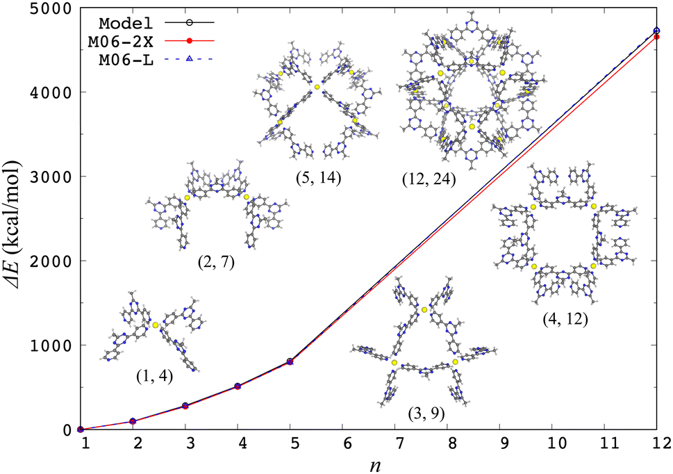 | ||
| Fig. 1 Single-point binding energies ΔE from the model Hamiltonian and the DFT calculations with two different functionals, where ΔE = E(PdnLm) + (4n − m)E(L) − nE(PdL4) at the crystal [Pd12L24]24+ and its partial [PdnLm]2n+ structures. Reproduced from Y. Yoshida, et al. Phys. Chem. Chem. Phys., 2021, 23, 866–877.39 | ||
The EHCF method, which also describes the electronic d–d states by construction, has been applied to computing structures and d–d excitations of wider range of transition metal complexes.18,19,21 For example, the EHCF approach combined with MM could successfully reproduce the structures and spin states of a wide range of Fe(II) and Co(II) complexes having mono- and poly-dentate nitrogen donor ligands.19,21 The EHCF has been also extended to periodic solids by incorporating effects from band structures, which was tested for the periodic transition metal oxides such as MnO.22
3 Molecular dynamics
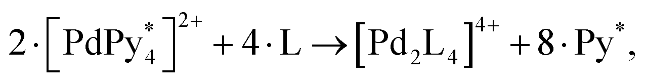
The relationship between complex reaction networks and energy landscapes has long been the subject of theoretical studies for structure prediction and extraction of molecular properties.40,41 Kinetic transition network12,42,43 provides a comprehensive description of transition processes and allows interpretation of molecular behaviors based on the energy landscape features. This is obtained as a mapping of the energy landscape or via MD data, with nodes and edges on the network corresponding to local minima and the transitions connecting them, respectively. This coarse-grained (CG) representation is very useful as a complementary approach to Monte Carlo and MD simulations. Visualization of the network is explicitly realized by using the so-called disconnectivity graph. This facilitates understanding the relationship between local minima, which are the lower ends of lines connected to each other at the lowest energy points (transition states).44,45 Based on this framework, thermodynamics and kinetics have been extensively discussed from atomic and molecular clusters,46,47 to CG models with rigid body components,48–50 condensed matter systems,51 biophysical systems,52,53 and of course assembly processes.54 Reaction rate constants can be calculated from conventionally used methods such as transition state theory, unimolecular kinetics, and direct dynamics calculations. Methodological and technical improvements in the kinetic transition network approach55–57 to extracting thermodynamic and kinetic properties can be incorporated into other methodological frameworks for the reaction network-based analysis.In the attempts to understand the self-assembly events, if it is possible to directly track and reproduce the global reaction process in computers, formation process of a certain geometrical structure can be visually captured. MD simulations would be adopted as the best way to such a purpose. In spite of the long and steady methodological development, MD studies on the coordination self-assembly started only recently, with one of the pioneering works published by Yoneya and co-workers in 2012.58 They selected an M6L8 nanosphere as a target system and demonstrated that over the course of simulations the spontaneous formation of the final product could be successfully observed.
To track the formation process of a nanosphere of octahedral symmetry composed of six Pd(II) ions and eight tritopic ligands, they specifically took the following procedures: (i) CaDA model was applied, in which four identical dummy atoms are coplanary attached to the Pd(II) ions. In this model the atomic charge of the Pd(II) cation is transferred to those four dummy atoms. Although the M–L binding in this model is purely electrostatic and too simple to represent the reality, in this study the simulation was performed with this model to propose the minimum model for the M6L8 self-assembly. (ii) A flexible united-atom model was applied for the tritopic ligand, with the exception of all the bonds being fixed to those at the equilibrium. (iii) They treat the solvent implicitly as a continuum medium to accelerate the assembly of metals and ligands to fill the time scale gap between the simulation and the reality. The combination of the Langevin dynamics (dynamic effects of the solvent molecules are taken into account), reaction fields (electrostatic effects of the solvent is represented by extending the classic reaction field method to ionic systems), and CG potentials (for van der Waals potential between ligands to be effectively short-range repulsive) was applied. It was found that the simulation results correlate well with the corresponding experimental ones, and that the difference in the lifetime between small-sized incomplete clusters and the completed M6L8 complex is crucially important in this self-assembly.
Subsequently, Yoneya and co-workers performed MD simulations and demonstrated the spontaneous formation for a M12L24 spherical complex.59 One of the contrast to the M6L8 is that they found the existence of kinetic traps with lower number of metal nuclei such as M6L12, M8L16, and M9L18. Their study made it clear that it is important to consider the kinetic factor in the self-assembly process of the larger complex. Behaviors of kinetic traps are strongly dependent on the bend angle of the ligand and the M–L bonding strength. It should be noted that the self-assembly processes identified in their simulations are used as a reference for running even larger MD simulations.60
Motivated by the above pioneering studies, and highlighting the importance of the function of the self-assembled structure as a molecular container, Jiang et al. presented an MD simulation to investigate the encapsulation of C60 and C70 fullerenes during the self-assembly process of a M2L4 nanocapsule that is self-assembled by the coordination of Hg cations and bent ditopic ligands.61 Stepwise formation of the nanocapsule and competitive fullerene encapsulation during dynamic structural changes in the self-assembly were detected successfully. This work helps design new functional nanomaterials capable of guest encapsulation and release.
Here we briefly mention the MD simulations for MOF or PCP (porous coordination polymer) and the nanocube, by viewing them as analogous systems in the context of tracking the molecular self-assembly process. In the MOF structure, vertices composed of single metal ions or ion clusters are linked by organic ligands. MOF is an important class of nanoporous materials because of its structural and functional properties, including the catalytic activity and the abilities for energy and gas storage. On the establishment of the design strategies for this artificial material, especially in mimicking the high-efficiency natural counterparts, a well-suited design of both the metal ion and the ligand is highly required. Although there are only a few works performed for obtaining the information about the growth process, knowing the details of (self-)organization processes and their mutual relations in time and space of various levels are getting more and more important. In a pioneering MD simulation for the growth process of MOF,62 the model developed for the MD study of the Pd12L24 complex was applied to MOF, by using the CaDA and the CG solvent models. Self-assembly simulations for the two- and three-dimensional MOFs were performed by modeling the M–L bond with the Coulomb potential. The simulation of the two-dimensional MOF self-assembly led to the identification of the range of the dielectric constant in the near-field to achieve regular networks. For the three-dimensional case, they tried to reveal the design factor for realizing regular 3D MOF. By keeping in mind the uncertainty of how the self-assembly process is affected by the continuum solvent model, Biswal et al. conducted systematic and comprehensive researches on the MOF self-assembly having Zn ion. In one study,63 they considered the models with different system size and the solvent types, succeeded the assembly of several two-dimensional layered network-like square arrangements, characterized the multistep assembly processes, and identified different geometrical structure of transient intermediates. In the other work,64 model-dependence of the structural behaviors in the self-assembly process was examined on the different Zn-ion, solvent, and ligand models. From their exhaustive analysis it was found that the model should be carefully chosen in the research of the MOF self-assembly.
Nanocube is a hexameric self-assembled structure of six gear-shaped amphiphile molecule, and it has about 1 nm-sized inner space, in which hydrophobic guest molecules can be encapsulated. Although possessing a highly ordered structure, in this compound less directional interactions such as van der Waals and hydrophobic effects play important roles. Some nanocubes are reported to exhibit a very high stability beyond the boiling point of water. An MD simulation for the self-assembly process of the nanocube was performed by Harada et al.65 In their study, by using an enhanced sampling technique instead of the conventional MD simulation, self-assembly process was inferred with the dissociation pathways from the hexameric nanocube form to six monomers in a stepwise manner. They also observed the stability of intermediate oligomers and predicted which process is the rate-determining step during the nanocube formation process. Yamamoto et al. focused on the solvent effect in the molecular level, and computationally examined the self-assembly mechanism in aqueous methanol solution.66 Starting from the all-atom total free energy calculation and evaluating the aggregation free energy for the partial cluster states, with the use of replica exchange with solute tempering, it was demonstrated from MD simulations that a highly ordered nanocube structure can be reproduced from the disordered state of the substrates. They also succeeded in offering the insights of the intermediates and encapsulated molecules in the atomistic level. A subsequent study with the newly developed implicit solvent model was performed by Imamura et al. for capturing the nanocube self-assembly process more comprehensively.67 While it was found that the CG model, which is more advantageous than all-atom model in the calculation efficiency, reasonably explains the solvent effect, the standard CG-MD simulation failed the reproduction of the nanocube structure. On the other hand, replica exchange CG-MD simulation successfully reproduced a highly ordered nanocube structure. Trajectory analysis revealed the transition network, and the main reaction pathways were identified. Finally, although we have focused on the ‘self-assembly process’ of the nanocube here, it should be noted that Tachikawa et al. also reported the simulation on the same system. In their MD studies, thermodynamic, structural and dynamic properties of the nanocubes and the factors that affect them have been elaborately investigated.68–71
One of the most advantageous points in the MD simulation is the visualization of the reaction process, especially the formation of the specific structure in the self-assembly process. MD simulations have also been used in the tracking of the self-organization of virus capsids (one of the simplest examples of the self-assembly in biology), with some ways of simplification and CG being necessary because of the large size.72 Coordination self-assembly system is more suitable for the MD studies than viral capsids, in that the simpler constituents and the smaller sizes enables the more direct and realistic modeling and unambiguous reaction analysis. However, serious difficulties are still remaining in realizing the time scale of the actual formation of self-assembled structure (second to hour or longer) being very large compared with that accessible in common MD simulations. Some devices and CG procedures are necessary to speed up the simulations.
4 QASAP-NASAP approach
As mentioned in Introduction, the research field of the molecular self-assembly is taking a step from looking only at the objective products under thermodynamic control to actively (kinetically) controlling reaction pathways by modulating the energy landscape. For realizing it in laboratories, it is useful to survey the entire reaction network to capture the information about important events occurring on it, that is, the dominant pathways, the rate-determining step, and kinetic traps and so on. In this section we introduce such attempts, emphasizing the interactive feedback between experimental and computational studies.4.1 QASAP-NASAP studies
In 2014, Hiraoka and co-workers developed QASAP (quantitative analysis of self-assembly process), a method for clarifying the reaction process of coordination self-assembly consisting of a metal ion M and a multitopic ligand L.73–75 QASAP was established as an experimental method to follow the reaction process of self-assembling complexes via tracking the time evolution of the average composition of the transiently formed intermediates in complex reactions, and has been used to elucidate the reaction process of coordination self-assembly of MmLn-type complexes with over 20 different geometric structures.76–94 Any intermediates of the coordination self-assembly can be indicated by MaLbXc (a, b, and c are 0 or positive integer, and note that the valence of ion is omitted here). QASAP focuses on the following two quantities calculated from a, b, and c,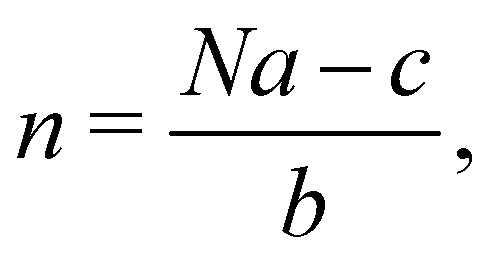 | (5) |
 | (6) |
The advent of QASAP lifted the research of the molecular self-assembly up to one step higher in that the reaction process became accessible via the average composition of intermediate species. Currently this method is being expanded to the systems with other than transition metal ions and multi-step reactions under operative kinetic control. As mentioned above, however, there are limits to what can be obtained from experimental studies alone. NASAP (numerical analysis of self-assembly process) was devised as the other wheel for the coordination self-assembly to complement this deficiency with numerical simulations. NASAP is basically composed of the following procedure: (i) constructing a reaction network from the substrates to the objective products for each target self-assembly system. To what extent the reaction network covers (i.e., how many chemical species and elementary reactions among them are included) is determined from the knowledge of the corresponding experiments. (ii) Assigning a reaction rate constant to each elementary reaction present in the network. In most cases the similar reactions are classified into the same reaction type having the same parameter values, because it is practically impossible to assign different rate constant to each elementary reaction in the case the reaction network is large as in the molecular self-assembly. (iii) Fitting of the simulated results to the experimentally available data by changing (sweeping) the rate constant values in certain specified numerical ranges. For the numerical fitting in which all the elementary reactions are classified into m classes, a numerical search in the m dimensional parameter space is performed. (iv) Running refined calculations with the set of rate constant which gives a well-fitted result to the experimental counterpart and obtaining the information of the reaction process such as the time evolution of each molecular species and the number of each reaction that occurred.
Fig. 2 presents a brief overview of the geometrical structures investigated by NASAP studies. Eight self-assembly systems with six geometries have been numerically analysed in detail based on the corresponding QASAP data, though the library of QASAP-NASAP joint research is ongoingly growing with the self-assembly systems larger in the number and more extensive in the diversity. NASAP was originated by Matsumura et al.95 for the analysis of the octahedron-shaped [Pd6L8]12+ capsule composed of Pd(II) complex and tritopic ligand 1 (Fig. 2(a)),
| 6·[PdPy4]2+ + 8·1 → [Pd618]12+ + 12 Py. | (7) |
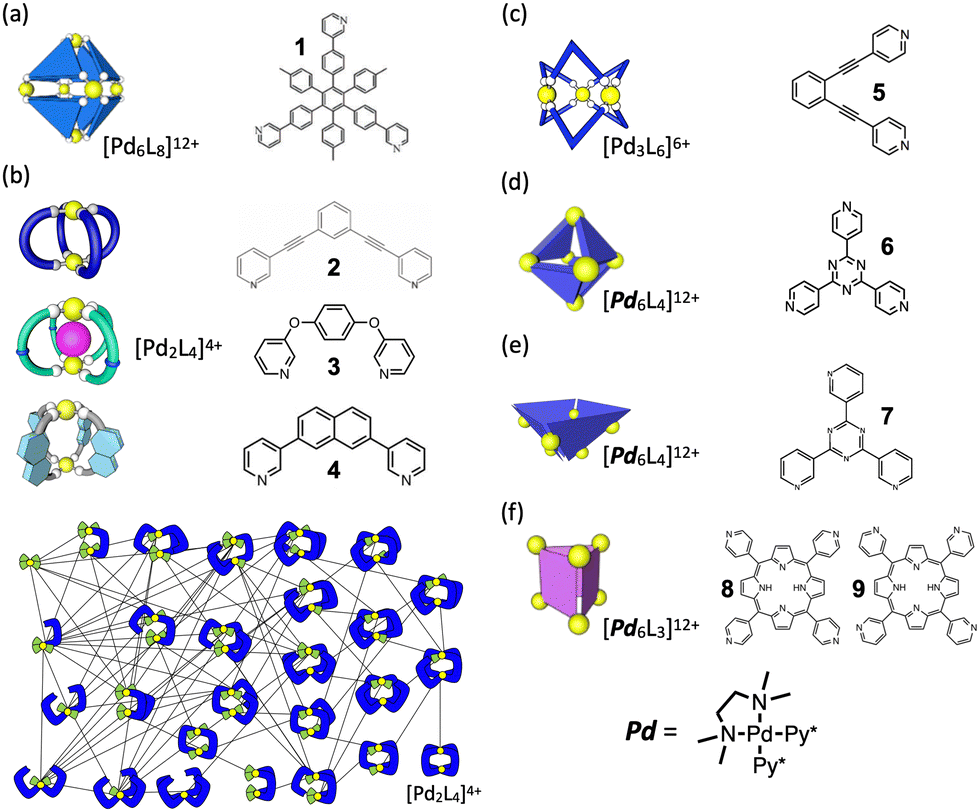 | ||
| Fig. 2 Geometrical structures of the metal-organic coordination complexes whose self-assembly processes were investigated by NASAP so far. Multitopic ligand used to construct each self-assembly is also indicated. (a) [Pd6L8]12+ capsule. (b) [Pd2L4]4+ cages, for which the reaction network employed in the simulations is shown. (c) [Pd3L6]6+ double-walled triangle. (d) [Pd6L4]12+ truncated tetrahedron. (e) [Pd6L4]12+ square-based pyramid. (f) [Pd6L3]12+ prism. For (d)–(f) self-assemblies, the metal source Pd is cis-protected Pd(II) complex (Pd[TMEDA]2+) where two coordination sites of the Pd(II) ion are occupied by a chelate ligand (TMEDA: N,N,N′,N′-tetramethylethylenediamine). | ||
In this first application of NASAP, parts of the capsule structure (1 ≤ a ≤ 6) were considered as the intermediate species. More than 170![[thin space (1/6-em)]](https://www.rsc.org/images/entities/char_2009.gif) 000 structures were categorized based on their composition, and a reaction network of 155 chemical species was constructed. Based on the experimental results that in spite of being the reactant in the final capsule formation ([Pd618Py]12+ → [Pd618Py]12+ + Py) the 1H NMR of [Pd618Py]12+ did not appear, two conformational isomers of [Pd618Py]12+ in slow dynamic equilibrium were explicitly included in their analysis. All the elementary reactions in the network were classified into four types. They divided the entire self-assembly reaction into three stages and discussed the time evolution of the intermediate species, with the dominant ones being (1) linear oligomers at the initial stage, (2) intramolecular Pd-1 bonds saturated at the middle stage, and (3) kinetic trapping state at the final stage. The time evolution detected in the corresponding experiment was properly reproduced with the timescale from millisecond to hours.
000 structures were categorized based on their composition, and a reaction network of 155 chemical species was constructed. Based on the experimental results that in spite of being the reactant in the final capsule formation ([Pd618Py]12+ → [Pd618Py]12+ + Py) the 1H NMR of [Pd618Py]12+ did not appear, two conformational isomers of [Pd618Py]12+ in slow dynamic equilibrium were explicitly included in their analysis. All the elementary reactions in the network were classified into four types. They divided the entire self-assembly reaction into three stages and discussed the time evolution of the intermediate species, with the dominant ones being (1) linear oligomers at the initial stage, (2) intramolecular Pd-1 bonds saturated at the middle stage, and (3) kinetic trapping state at the final stage. The time evolution detected in the corresponding experiment was properly reproduced with the timescale from millisecond to hours.
Motivated by the successful reproduction and analysis of the QASAP result, NASAP has been sophisticated step by step in obtaining the information of the main reaction pathways, the rate-determining step, and the kinetic traps. In the following subsections we show the results of QASAP-NASAP studies.94
 | (8) |
1. Cage formation with rapid ligand consumption. For the first case, QASAP clearly indicated that the consumption of the ditopic ligand 2 was too fast for the very initial stage of the self-assembly to be unobservable.78 NASAP was performed for this system with the reaction network having 29 chemical species and 68 elementary reactions among them, each of which has both forward and backward directions.96 All the elementary reactions were classified into four types based on the similarity of reaction behavior as follows:
1. Intermolecular ligand exchange reaction with a free ligand 2: k1f [min−1 M−1] and k1b [min−1 M−1] are defined for the forward and the backward reactions, respectively.
2. Formation of dinuclear species from two mononuclear ones: k2f [min−1 M−1] and k2b [min−1 M−1] for the forward and the backward, respectively.
3. Intramolecular ligand exchange reaction in dinuclear species: k3f [min−1] and k3b [min−1 M−1] for the forward and the backward, respectively.
4. Cage completion: k4f [min−1] and k4b [min−1 M−1] for the forward and the backward, respectively.
Rate-determining step was clearly identified as the final stage of the self-assembly (cage completion step). NASAP have also shown the reaction behaviors at the initial stage of the self-assembly, which was not unclear with QASAP alone.
2. Kinetic template effect to avoid sheet formation. In the second application of NASAP to Pd2L4 cage, kinetic template effect of counter anion was confirmed in the self-assembly of ditopic ligand 3 and Pd(II) source [PdPy*4](OTf)2. For this self-assembly, QASAP revealed the reaction pathway was largely affected by the counter anions.97 Without template anion (NO3−), a micrometer-sized sheet is kinetically trapped (off-pathway), which is converted into the thermodynamically most stable cage by the template anion. When NO3− is present from the start, the cage is selectively produced by the preferential cyclization of a dinuclear intermediate (on-pathway).
For the QASAP results in which the fact that the NO3− anion promotes the reactions in the early stage of the self-assembly to a greater extent than those in the final step was extracted, NASAP simulation was conducted with the same reaction network as that used for [Pd224]4+ and a little sophisticated classification of reaction types, in which the intramolecular reaction was separated into two types (the first and the second bridgings). The simulation results were found to support the strong kinetic template effect on the on-pathway, showing that the rate constants of the intramolecular cyclization in the early stage of the self-assembly (k3 and k4) are larger than that in the final step (k5).
3. Navigated self-assembly of Pd 2 L 4 cage with the modulation of energy landscape. In this study, the formation of a thermodynamically metastable [Pd244]4+ cage structure composed of naphthalene-based ditopic ligands (L) and Pd(II) was tracked with both QASAP and NASAP.98 This is an example of kinetically controlled molecular self-assembly found in a Pd2L4 cage system. In the case without the guest anion (BF4−) large intermediate species are formed, while with the guest anion the self-assembly proceeds to not the thermodynamically most stable species but a metastable [Pd244]4+ cage, with the anion being encapsulated in it. The self-assembly process to the cage was found to be navigated by the reaction condition with the counter anion BF4− in weak coordinative solvent CD3NO2 to modulate energy landscape, with the decomposition into the thermodynamical state being prevented. Also in this case, NASAP with the same setup as for [Pd234]2+ successfully reproduced the corresponding QASAP results and indicated the navigated reaction pathway to the objective structure.
Starting from the numerical reproduction of the corresponding QASAP results,87 NASAP specified what causes a balance among the participating elementary chemical reactions, that is, oligomerization, double-wall making (d) and cyclization (c), in the self-assembly process. It was found that the numbers of isomers having the same composition and reaction points available in them and their mutual relations determine the reaction trends and time ordering in the entire self-assembly process. More specifically, for this Pd3L6 DWT system the self-assembly process was found to proceed as d-c-d-d after the formation of oligomers with a proper length.
This study is the first example for demonstrating another utility of the network model created in NASAP for predicting experimental results under kinetic conditions. The outcomes of self-assembly depending on the stoichiometric ratio under kinetic control were predicted by numerical simulations with the rate constants fixed by NASAP, which are well consistent with the experimental results in a certain range of the initial stoichiometric ratio of the substrates ([L]0/[Pd]0), indicating that numerical simulation in a reaction network model is a powerful approach to find an appropriate reaction condition to produce a desired assembly under kinetic control.
1. Pd 6 L 4 truncated tetrahedron. (TT) In this QASAP-NASAP joint study, the self-assembly processes of octahedron-shaped Pd6L4 cages (truncated tetrahedron, TT) consisting of cis-protected Pd(II) complexes and two kinds of organic tritopic ligands were investigated100 (Fig. 2(d)). Considering that whether large kinetically trapped species are produced or not is determined by the balance between the oligomerization and the cyclization, the formation of such kinetically trapped species is due to the over oligomerization.
QASAP and NASAP (NASAP is applied to one of the ligands, 6) indicate that the cyclization is slower than the oligomerization and the cross-linking in the self-assembly of the [Pd664](BF4)12 cage. NASAP was performed with the reaction network with 56 chemical species connected with 249 elementary reactions, each of which has the forward and the backward reactions. All the reactions were classified into three types, that is, oligomerization, cyclization, and cross-linking in a formed cycle, for the purpose of describing the process with as small number of parameters to obtain a clear picture as possible. NASAP indicated that the cyclization reactions mainly take place from the linear intermediates and that the relative difference in the rate constants between the oligomerization (koligo) and the crosslinking (kcross-link) does not affect the trend of the self-assembly process of the [Pd664](BF4)12 cage. Although a simple comparison between parameter values of the first-order (intramolecular) and the second-order (intermolecular) reactions seems a little too simplistic, this study exemplifies that in some cases many useful insights are accessible even for the not-too-small-sized objective product without too many and complicated classification of elementary reactions.
2. Pd 6 L 4 square-based pyramid (SP). In the QASAP-NASAP joint study for another Pd6L4 structural isomer101 (Fig. 2(e)), it was confirmed that the self-assembly process is not as simple as can be expected from the final assembly structure and its components. The target is the self-assembly of a Pd674 square-based pyramid (SP) composed of six cis-protected Pd(II) complexes (M) and four triangular tritopic ligands (7). A numerical analysis of the experimental data based on a reaction network model where 579 reactions between the possible 112 species were considered revealed the self-assembly pathways to one of the two M6L4 isomers, the other of which is the TT isomer as a possible product.
In this study, the intermediate [Pd272Py*]4+, (2,2,1) in a shorthand notation with suffices a, b, and c, was found to be the key species. If (2,2,1) is transformed to (2,2,0) via intramolecular reaction, it is a kinetic trap. Intermolecular reaction of (2,2,1) with (2,1,2) lead to the pathway to form (6,4,0) SP. NASAP has also clearly confirmed the main reaction pathway not through the expected route from the structure of intermediates.
From this study, contrary to common intuition, it was found that for both 8 and 9 macrocyclization (c) takes faster than bridging reaction (b), with the ordering being c-b-b-b after oligomerization. Bridging reaction prior to macrocyclization tended to lead to kinetically trapped species, and the relative magnitude of the rate constants between those two kinds of intramolecular reactions was found to be the key factor.
4.2 Comments on the numerical approach used for the kinetic study and related studies
In all the NASAP simulations performed so far, which were introduced in sequence as above, the time evolution of elementary chemical reactions are numerically followed in a stochastic manner, and more specifically, by using the so-called Gillespie algorithm.103–106 The Gillespie algorithm is one of the kinetic Monte Carlo (kMC) methods, which is implemented from the related stochastic master equation. In the kMC algorithm the time evolution of complex many-particle systems is simulated according to the frequency or transition probability of each event based on the kinetic and procedural information of elementary process and mechanism, through generating random numbers.This method is widely used in physics, chemistry, biology and engineering. Bortz et al. introduced this as a reorganization of the standard Monte Carlo algorithm for the Ising model,107 in which choices of random configurational transitions are biased according to each transition's likelihood in such a way that transitions which are easy to occur are chosen preferentially. D'orsagna and co-workers simulated and analysed the nucleation and molecular aggregation.108,109 Comparison with the classic equilibrium equation was shown, and they discussed the differences between them. They indicated the finite-size effect not considered in the mass-balance equation. Master equation approach is also applied to the chemical reactions in gas phase represented by combustion chemistry, with those related to multiple potential wells and connections among them kept in mind.110,111 Biochemical reactions are also within the scope of successful application of the stochastic method, including single-molecule enzyme,112 transcriptional regulation,113 self-assembly of virus capsids,114 and so on. Battaile shows an application example of the kMC method in engineering, that is, an attempt to reveal a potential mechanism of grain refinement during the deposition of polycrystalline thin films, with careful explanation for the overview of background theory.115
In the static kMC method whose examples are listed above, unlike the so-called on-the-fly kMC approaches where possible reaction pathways are produced in a self-developing manner,116,117 it is necessary to prepare event lists in which all the expected states and reactions are determined in advance and the rates and thermodynamics are obtained from the prepared network. However, this framework enables us to conduct analysis based on the discrete pathway sampling approach, where all the pathways are obtained from geometry optimization, with the post-processing resorting to statistical mechanics and unimolecular rate theory being possible.118,119
It is widely known that the chemical reactions represented with the simultaneous equations can be solved (i.e., the time evolution of the molecules supposed to participate in the global chemical reaction can be tracked) by using the ordinary differential equations (ODE). Although we cite only a few references here,120–122 there is a vast number of articles employing ODE for tracking chemical reactions. The present authors also used the ODE algorithm for tracking the time evolution of a smaller model chemical reactions for the ligand exchange at the very beginning of NASAP project and argued both the similarity and the difference upon the comparison of the numerical results with those from the Gillespie algorithm.123 For the large molecular numbers as considered in the NASAP studies (QASAP experimental condition) the same reaction behaviors are available, regardless of the computational methods used. The main reason for resorting to the stochastic method in the QASAP-NASAP studies is the countability of both the molecular numbers present in the simulation box and the elementary reactions occurred. While the ODEs only give us a continuous and relatively smooth time evolution of the “concentration” of each intermediate molecule, the stochastic algorithm enables us to know when one of the possible reactions takes place under what circumstances (i.e., distributions of other species). This is one of advantages for the NASAP to analyse and interpret which reaction pathways the particular self-assembly reaction pass through, because a sequence of a simply counting the reaction frequency (occurred number) for each elementary reaction and the corresponding molecular numbers (increase and decrease) related to that reaction automatically leads to the dominant reaction pathways to the final self-assembly product without the misinterpretation of kinetic traps as the dominant species on the main reaction pathway.
Incidentally, although we refrain listing up all the contributions here in this article, there is a vast number of studies on various kinds of polymerization and supramolecular polymerization reaction with both the stochastic and the deterministic approaches. For the polymerization reaction we cite a review article.124 And two articles are referred to for the mathematical analysis of supramolecular polymerization,125,126 in both of which the analysis was performed with both the deterministic and stochastic ways, thereby providing solid ground for their results.
5 Conclusions and outlook
In this perspective article, three approaches were mainly reviewed to unveil the mechanism of self-assembly at the molecular level. One is the semi-quantum chemical Hamiltonian approach to efficiently describe the bond formation of M–L related to the local character of the energy landscape. The second is the molecular dynamics (MD) simulation, which allows to directly track the reaction process. And the third approach is NASAP, a complementary tool for QASAP, to grasp the global aspects of self-assembly. Contributions by the present authors were made mainly for the first and the third approaches, in which theoretical and computational methods were confirmed to play successful roles in understanding and interpreting the self-assembly pathways and inspecting energy landscapes of reaction, from both a local (semi-quantum chemical) and a broader (time evolution of species concentration) points of view. Studies on their lines are extending to the prediction and the presentation of guiding principles for the experimental works related to the topics mentioned below, and those results will be shown elsewhere. It should be noted that most referred researches that are related to the present authors have been performed almost in parallel between experiment and theory. By collaboratively proceeding the research in this way, those studies have been performed successfully with less time lags between them, creating a positive feedback loop. With the knowledge of the energy landscape in hand, it may be possible to make a strategy of skillfully performing the molecular self-assembly under kinetic control.Finally, we would like to comment on perspectives beyond the thermodynamic treatment for more active control of the system. Many molecular self-assemblies proceed under thermodynamic control based on reversible chemical bonds between components. The main advantage of this is that even if incorrect bonds are formed between components, the reversibility of the bonds allows them to be repaired, and finally the structure which is thermodynamically the most stable is preferred. For this reason, molecular self-assembly in many artificial systems (especially those forming discrete structures) has been conducted with the thermodynamically controlled condition. Under such a situation, the Boltzmann distribution reflects the free energy difference (ΔG) between products. Since the free energy is a state function, the consequences of self-assembly are independent of the reaction pathway. However, the molecular self-assembly under thermodynamic control is restricted by the Boltzmann distribution and is not almighty, because (1) the thermodynamically most stable products cannot be produced with the yield more than that in the Boltzmann distribution, and (2) metastable species can never be preferentially generated. An example of the limit of the self-assembly under thermodynamic control can be seen in a multicomponent metallo-organic coordination self-assembly consisting of several types of ligands.127–132 Coordination self-assembly is a topic of increasingly more interest these days. Even in the self-assembly of a relatively simple M2L4 cage structure consisting of two M and four L, it is not easy to form specific cage complexes from multiple species of ditopic ligands in a thermodynamically controlled manner.133 This is because as the number of component types increases, various isomers with close thermodynamic stability are formed, and it is difficult to preferentially produce a single assembly under thermodynamic control.
It has been made clear that in many cases (especially, biological systems) we often observe the kinetically trapped species during self-assembly with a long lifetime.134–137 This means that nature skillfully uses kinetics by constructing multicomponent assemblies that cannot be constructed under thermodynamic control, through pathway dependence. And it is also possible to find through experimental studies of coordination self-assembly processes that when molecular self-assembly is carried out under certain conditions, the system as a whole exhibits directionality with maintaining locally reversible nature, and that the products are not Boltzmann distributed. These facts indicate that we cannot understand natural phenomena with the simple scheme of reversible bonding being identical to chemical equilibrium, and that there exists a world with irreversibility created from reversible bonding. In such a case we can carry out the molecular self-assembly under kinetic control with pathway selection, and the understanding of the reaction mechanism becomes essential for realizing pathway dependent molecular self-assembly. In the case of molecular self-assembly, however, the relation among the elementary reactions is largely from the textbook reaction and simple polymerization schemes, and necessarily expressed as a form of complex network, with the chemical species and reactions being the nodes and edges, respectively.
Author contributions
Satoshi Takahashi: writing – original draft (equal). Satoru Iuchi: writing – original draft (equal). Shuichi Hiraoka: conceptualization (equal); funding acquisition (equal); project administration (equal); supervision (equal); writing – review & editing (equal). Hirofumi Sato: conceptualization (equal); funding acquisition (equal); project administration (equal); supervision (equal); writing – review & editing (equal).Conflicts of interest
There are no conflicts to declare.Acknowledgements
We are grateful for all the collaborators, including Dr Yoshihiro Matsumura, Yuichiro Yoshida, and Tomoki Tateishi. A series of works was supported by JSPS KAKENHI (Grant No. JP16K05511, JP17H03009, JP20K05417, JP21K18974). Theoretical computations were partly performed in the Research Center for Computational Science, Okazaki, Japan.Notes and references
- D. J. Kushner, Bacteriol. Rev., 1969, 33, 302–345 CrossRef CAS PubMed.
- G. M. Whitesides, J. P. Mathias and C. T. Seto, Science, 1991, 254, 1312–1319 CrossRef CAS PubMed.
- G. M. Whitesides and B. Grzybowski, Science, 2002, 295, 2418–2421 CrossRef CAS PubMed.
- S. Zhang, Nat. Biotechnol., 2003, 21, 1171–1178 CrossRef CAS PubMed.
- A. Tarzia and K. E. Jelfs, Chem. Commun., 2022, 58, 3717–3730 RSC.
- T. K. Piskorz, V. Martí-Centelles, T. A. Young, P. J. Lusby and F. Duarte, ACS Catal., 2022, 12, 5806–5826 CrossRef CAS PubMed.
- R. J. Deeth, A. Anastasi, C. Diedrich and K. Randell, Coord. Chem. Rev., 2009, 253, 795–816 CrossRef CAS.
- I. Horvath, D. J. Wales and S. N. Fejer, Nanoscale Adv., 2022, 4, 4272–4278 RSC.
- I. G. Johnston, A. A. Louis and J. P. K. Doye, J. Phys.: Condens. Matter, 2010, 22, 104101 CrossRef PubMed.
- D. J. Wales and T. V. Bogdan, J. Phys. Chem. B, 2006, 110, 20765–20776 CrossRef CAS PubMed.
- D. J. Wales, Philos. Trans. R. Soc., A, 2005, 363, 357–377 CrossRef CAS PubMed.
- D. J. Wales, Curr. Opin. Struct. Biol., 2010, 20, 3–10 CrossRef CAS PubMed.
- S. Grimme, C. Bannwarth and P. Shushkov, J. Chem. Theory Comput., 2017, 13, 1989–2009 CrossRef CAS PubMed.
- C. Bannwarth, S. Ehlert and S. Grimme, J. Chem. Theory Comput., 2019, 15, 1652–1671 CrossRef CAS PubMed.
- B. N. Figgis and M. A. Hitchman, Ligand Field Theory and Its Applications, Wiley, New York, 2000 Search PubMed.
- S. Iuchi, A. Morita and S. Kato, J. Chem. Phys., 2004, 121, 8446–8457 CrossRef CAS PubMed.
- S. Iuchi, J. Chem. Phys., 2012, 136, 064519 CrossRef PubMed.
- A. V. Soudackov, A. L. Tchougreeff and I. A. Misurkin, Theor. Chim. Acta, 1992, 83, 389–416 CrossRef.
- A. L. Tchougréeff, A. V. Soudackov, J. van Leusen, P. Kögerler, K.-D. Becker and R. Dronskowski, Int. J. Quantum Chem., 2016, 116, 282–294 CrossRef.
- C. E. Schäffer and C. K. Jørgensen, Mol. Phys., 1965, 9, 401–412 CrossRef.
- M. B. Darkhovskii and A. L. Tchougréeff, J. Phys. Chem. A, 2004, 108, 6351–6364 CrossRef CAS.
- I. Popov, E. Plekhanov, A. Tchougréeff and E. Besley, Mol. Phys., 2022, e2106905 CrossRef.
- P. Li and K. M. Merz Jr., Chem. Rev., 2017, 117, 1564–1686 CrossRef CAS PubMed.
- S. Spicher and S. Grimme, Angew. Chem., Int. Ed., 2020, 59, 15665–15673 CrossRef CAS PubMed.
- J. G. Brandenburg, C. Bannwarth, A. Hansen and S. Grimme, J. Chem. Phys., 2018, 148, 064104 CrossRef PubMed.
- S. Spicher, M. Bursch and S. Grimme, J. Phys. Chem. C, 2020, 124, 27529–27541 CrossRef CAS.
- M. Bursch, H. Neugebauer and S. Grimme, Angew. Chem., Int. Ed., 2019, 58, 11078–11087 CrossRef CAS PubMed.
- R. J. Deeth and L. J. A. Hearnshaw, Dalton Trans., 2006, 1092–1100 RSC.
- R. J. Deeth, D. L. Foulis and B. J. Williams-Hubbard, Dalton Trans., 2003, 3949–3955 RSC.
- R. J. Deeth, N. Fey and B. Williams-Hubbard, J. Comput. Chem., 2005, 26, 123–130 CrossRef CAS PubMed.
- P. Melix, F. Paesani and T. Heine, Adv. Theory Simul., 2019, 2, 1900098 CrossRef CAS.
- J. Cirera, V. Babin and F. Paesani, Inorg. Chem., 2014, 53, 11020–11028 CrossRef CAS PubMed.
- C. E. Schäffer, C. Anthon and J. Bendix, Coord. Chem. Rev., 2009, 253, 575–593 CrossRef.
- S. K. Singh, J. Eng, M. Atanasov and F. Neese, Coord. Chem. Rev., 2017, 344, 2–25 CrossRef CAS.
- L. Lang, M. Atanasov and F. Neese, J. Phys. Chem. A, 2020, 124, 1025–1037 CrossRef CAS PubMed.
- M. Buchhorn, R. J. Deeth and V. Krewald, Chem. – Eur. J., 2022, 28, e202103775 CAS.
- Y. Matsumura, S. Iuchi and H. Sato, Phys. Chem. Chem. Phys., 2018, 20, 1164–1172 RSC.
- Y. Matsumura, S. Iuchi, S. Hiraoka and H. Sato, Phys. Chem. Chem. Phys., 2018, 20, 7383–7386 RSC.
- Y. Yoshida, S. Iuchi and H. Sato, Phys. Chem. Chem. Phys., 2021, 23, 866–877 RSC.
- D. J. Wales, Annu. Rev. Phys. Chem., 2018, 69, 401–425 CrossRef CAS PubMed.
- D. J. Wales, J. Chem. Phys., 2015, 142, 130901 CrossRef CAS PubMed.
- F. Noé and S. Fischer, Curr. Opin. Struct. Biol., 2008, 18, 154–162 CrossRef PubMed.
- D. Prada-Gracia, J. Gómez-Gardeñes, P. Echenique and F. Fernando, PLoS Comput. Biol., 2009, 5, e1000415 CrossRef PubMed.
- O. M. Becker and M. Karplus, J. Chem. Phys., 1997, 106, 1495–1517 CrossRef CAS.
- D. J. Wales, M. A. Miller and T. R. Walsh, Nature, 1998, 394, 758–760 CrossRef CAS.
- F. Calvo, J. P. K. Doye and D. J. Wales, Nanoscale, 2012, 4, 1085–1100 RSC.
- D. Schebarchov, F. Baletto and D. J. Wales, Nanoscale, 2018, 10, 2004–2016 RSC.
- J. Hernández-Rojas, F. Calvo, S. Niblett and D. J. Wales, Phys. Chem. Chem. Phys., 2017, 19, 1884–1895 RSC.
- J. D. Farrell, C. Lines, J. J. Shepherd, D. Chakrabarti, M. A. Miller and D. J. Wales, Soft Matter, 2013, 9, 5407–5416 RSC.
- Y. Yoshida, H. Sato, J. W. R. Morgan and D. J. Wales, Chem. Phys. Lett., 2016, 664, 5–9 CrossRef CAS.
- J. W. R. Morgan, D. Mehta and D. J. Wales, Phys. Chem. Chem. Phys., 2017, 19, 25498–25508 RSC.
- J. A. Joseph, K. Röder, D. Chakraborty, R. G. Mantell and D. J. Wales, Chem. Commun., 2017, 53, 6974–6988 RSC.
- J. M. Carr and D. J. Wales, Phys. Chem. Chem. Phys., 2009, 11, 3341–3354 RSC.
- B. Barz, D. J. Wales and B. Strodel, J. Phys. Chem. B, 2014, 118, 1003–1011 CrossRef CAS PubMed.
- J. D. Stevenson and D. J. Wales, J. Chem. Phys., 2014, 141, 041104 CrossRef PubMed.
- D. J. Sharpe and D. J. Wales, J. Chem. Phys., 2019, 151, 124101 CrossRef PubMed.
- T. D. Swinburne and D. J. Wales, J. Chem. Theory Comput., 2020, 16, 2661–2679 CrossRef CAS PubMed.
- M. Yoneya, S. Tsuzuki, T. Yamaguchi, S. Sato and M. Fujita, ACS Nano, 2014, 8, 1290–1296 CrossRef CAS PubMed.
- M. Yoneya, T. Yamaguchi, S. Sato and M. Fujita, J. Am. Chem. Soc., 2012, 134, 14401–14407 CrossRef CAS PubMed.
- A. V. Zhukhovitskiy, M. Zhong, E. G. Keeler, V. K. Michaelis, J. E. P. Sun, M. J. A. Hore, D. J. Pochan, R. G. Griffin, A. P. Willard and J. A. Johnson, Nat. Chem., 2016, 8, 33–41 CrossRef CAS PubMed.
- Y. Jiang, H. Zhang, Z. Cui and T. Tan, J. Phys. Chem. Lett., 2017, 8, 2082–2086 CrossRef CAS PubMed.
- M. Yoneya, S. Tsuzuki and M. Aoyagi, Phys. Chem. Chem. Phys., 2015, 17, 8649–8652 RSC.
- D. Biswal and P. G. Kusalik, ACS Nano, 2017, 11, 258–268 CrossRef CAS PubMed.
- D. Biswal and P. G. Kusalik, J. Chem. Phys., 2017, 147, 044702 CrossRef PubMed.
- R. Harada, T. Mashiko, M. Tachikawa, S. Hiraoka and Y. Shigeta, Phys. Chem. Chem. Phys., 2018, 20, 9115–9122 RSC.
- T. Yamamoto, H. Are, S. Shanker, H. Sato and S. Hiraoka, J. Phys. Chem. Lett., 2018, 9, 6082–6088 CrossRef CAS PubMed.
- K. Imamura, T. Yamamoto and H. Sato, Chem. Phys. Lett., 2020, 742, 137135 CrossRef CAS.
- J. Koseki, Y. Kita, S. Hiraoka, U. Nagashima and M. Tachikawa, Int. J. Quantum Chem., 2013, 113, 397–400 CrossRef CAS.
- T. Mashiko, K. Yamada, T. Kojima, S. Hiraoka, U. Nagashima and M. Tachikawa, Chem. Lett., 2014, 43, 366–368 CrossRef CAS.
- T. Mashiko, K. Yamada, S. Hiraoka, U. Nagashima and M. Tachikawa, Mol. Simul., 2015, 41, 845–849 CrossRef CAS.
- T. Mashiko, S. Hiraoka, U. Nagashima and M. Tachikawa, J. Phys. Chem. B, 2019, 123, 5176–5180 CrossRef CAS PubMed.
- D. C. Rapaport, Phys. Biol., 2010, 7, 045001 CrossRef CAS PubMed.
- A. Baba, T. Kojima and S. Hiraoka, J. Am. Chem. Soc., 2015, 137, 7664–7667 CrossRef CAS PubMed.
- A. Baba, T. Kojima and S. Hiraoka, Chem. – Eur. J., 2018, 24, 838–847 CrossRef CAS PubMed.
- Y. Tsujimoto, T. Kojima and S. Hiraoka, Chem. Sci., 2014, 5, 4167–4172 RSC.
- S. Kai, Y. Sakuma, T. Mashiko, T. Kojima, M. Tachikawa and S. Hiraoka, Inorg. Chem., 2017, 56, 12652–12663 CrossRef CAS PubMed.
- S. Kai, T. Shigeta, T. Kojima and S. Hiraoka, Chem. – Asian J., 2017, 12, 3203–3207 CrossRef CAS PubMed.
- S. Kai, V. Marti-Centelles, Y. Sakuma, T. Mashiko, T. Kojima, U. Nagashima, M. Tachikawa, P. J. Lusby and S. Hiraoka, Chem. – Eur. J., 2018, 24, 663–671 CrossRef CAS PubMed.
- A. Baba, T. Kojima and S. Hiraoka, Chem. – Eur. J., 2018, 24, 838–847 CrossRef CAS PubMed.
- S. Kai, M. Nakagawa, T. Kojima, X. Li, M. Yamashina, M. Yoshizawa and S. Hiraoka, Chem. – Eur. J., 2018, 24, 3965–3969 CrossRef CAS PubMed.
- T. Tateishi, W. Zhu, L. H. Foianesi-Takeshige, T. Kojima, K. Ogata and S. Hiraoka, Eur. J. Inorg. Chem., 2018, 1192–1197 CrossRef CAS.
- T. Tateishi, T. Kojima and S. Hiraoka, Inorg. Chem., 2018, 57, 2686–2694 CrossRef CAS PubMed.
- S. Kai, S. P. Maddala, T. Kojima, S. Akagi, K. Harano, E. Nakamura and S. Hiraoka, Dalton Trans., 2018, 47, 3258–3263 RSC.
- T. Tateishi, T. Kojima and S. Hiraoka, Commun. Chem., 2018, 1, 20 CrossRef.
- S. Kai, T. Kojima, F. L. Thorp-Greenwood, M. J. Hardie and S. Hiraoka, Chem. Sci., 2018, 9, 4104–4108 RSC.
- M. Nakagawa, S. Kai, T. Kojima and S. Hiraoka, Chem. – Eur. J., 2018, 24, 8804–8808 CrossRef CAS PubMed.
- T. Tateishi, S. Kai, Y. Sasaki, T. Kojima, S. Takahashi and S. Hiraoka, Chem. Commun., 2018, 54, 7758–7761 RSC.
- S. Kai, T. Tateishi, T. Kojima, S. Takahashi and S. Hiraoka, Inorg. Chem., 2018, 57, 13083–13086 CrossRef CAS PubMed.
- S. Hiraoka, Isr. J. Chem., 2019, 59, 151–165 CrossRef CAS.
- S. Komine, T. Tateishi, T. Kojima, H. Nakagawa, Y. Hayashi, S. Takahashi and S. Hiraoka, Dalton Trans., 2019, 48, 4139–4148 RSC.
- T. Tateishi, Y. Yasutake, T. Kojima, S. Takahashi and S. Hiraoka, Commun. Chem., 2019, 2, 25 CrossRef.
- S. Hiraoka, Chem. Rec., 2015, 15, 1144–1147 CrossRef CAS PubMed.
- S. Hiraoka, Bull. Chem. Soc. Jpn., 2018, 91, 957–978 CrossRef CAS.
- S. Hiraoka, S. Takahashi and H. Sato, Chem. Rec., 2021, 21, 443–459 CrossRef CAS PubMed.
- Y. Matsumura, S. Hiraoka and H. Sato, Phys. Chem. Chem. Phys., 2017, 19, 20338–20342 RSC.
- S. Takahashi, Y. Sasaki, S. Hiraoka and S. Sato, Phys. Chem. Chem. Phys., 2019, 21, 6341–6347 RSC.
- L. H. Foianesi-Takeshige, S. Takahashi, T. Tateishi, R. Sekine, A. Okazawa, W. Zhu, T. Kojima, K. Harano, E. Nakamura, H. Sato and S. Hiraoka, Commun. Chem., 2019, 2, 128 CrossRef.
- T. Tateishi, S. Takahashi, A. Okazawa, V. Martí-Centelles, J. Wang, T. Kojima, P. J. Lusby, H. Sato and S. Hiraoka, J. Am. Chem. Soc., 2019, 141, 19669–19676 CrossRef CAS PubMed.
- S. Takahashi, T. Tateishi, Y. Sasaki, H. Sato and S. Hiraoka, Phys. Chem. Chem. Phys., 2020, 22, 26614–26626 RSC.
- S. Komine, S. Takahashi, T. Kojima, H. Sato and S. Hiraoka, J. Am. Chem. Soc., 2019, 141, 3178–3186 CrossRef CAS PubMed.
- T. Tateishi, S. Takahashi, I. Kikuchi, K. Aratsu, H. Sato and S. Hiraoka, Inorg. Chem., 2021, 60, 16678–16685 CrossRef CAS PubMed.
- X. Zhang, S. Takahashi, K. Aratsu, I. Kikuchi, H. Sato and S. Hiraoka, Phys. Chem. Chem. Phys., 2022, 24, 2997–3006 RSC.
- D. T. Gillespie, J. Comput. Phys., 1976, 22, 403–434 CrossRef CAS.
- D. T. Gillespie, J. Phys. Chem., 1977, 81, 2340–2361 CrossRef CAS.
- D. T. Gillespie, Phys. A, 1992, 188, 404–425 CrossRef CAS.
- D. T. Gillespie, Annu. Rev. Phys. Chem., 2007, 58, 35–55 CrossRef CAS PubMed.
- A. B. Bortz, M. H. Kalos and J. L. Lebowitz, J. Comput. Phys., 1975, 17, 10–18 CrossRef.
- M. R. D'Orsogna, G. Lakatos and T. Chou, J. Chem. Phys., 2012, 136, 084110 CrossRef PubMed.
- M. R. D'Orsogna, B. Zhao, B. Berenji and T. Chou, J. Chem. Phys., 2013, 139, 121918 CrossRef PubMed.
- J. A. Miller and S. J. Klippenstein, J. Phys. Chem. A, 2006, 110, 10528–10544 CrossRef CAS PubMed.
- M. J. Pilling and S. H. Robertson, Annu. Rev. Phys. Chem., 2003, 54, 245–275 CrossRef CAS PubMed.
- H. Qian and L. M. Bishop, Int. J. Mol. Sci., 2010, 11, 3472–3500 CrossRef CAS PubMed.
- T. B. Kepler and T. C. Elston, Biophys. J., 2001, 81, 3116–3136 CrossRef CAS PubMed.
- B. Sweeney, T. Zhang and R. Schwartz, Biophys. J., 2008, 94, 772–783 CrossRef CAS PubMed.
- C. C. Battaile, Comput. Methods Appl. Mech. Engrg., 2008, 197, 3386–3398 CrossRef.
- H. Xu, Y. N. Osetsky and R. E. Stoller, Phys. Rev. B: Condens. Matter Mater. Phys., 2011, 84, 132103 CrossRef.
- X. Guo, D. Minakata and J. Crittenden, Environ. Sci. Technol., 2015, 49, 9230–9236 CrossRef CAS PubMed.
- D. J. Wales, Mol. Phys., 2002, 100, 3285–3305 CrossRef CAS.
- D. J. Wales, Int. Rev. Phys. Chem., 2006, 25, 237–282 Search PubMed.
- R. E. Glaser, M. A. Delarosa, A. O. Salau and C. Chicone, J. Chem. Educ., 2014, 91, 7 CrossRef.
- W. S. Hlavacek, A. Redondo, C. Wofsy and B. Goldstein, Bull. Math. Biol., 2002, 64, 887–911 CrossRef CAS PubMed.
- P. Moisant, H. Neeman and A. Zlotnick, Biophys. J., 2010, 99, 1350–1357 CrossRef CAS PubMed.
- T. Iioka, S. Takahashi, Y. Yoshida, Y. Matsumura, S. Hiraoka and S. Sato, J. Comput. Chem., 2019, 40, 279–285 CrossRef CAS PubMed.
- E. Saldívar-Guerra, Macromol. React. Eng., 2020, 14, 2000010 CrossRef.
- A. J. Markvoort, H. M. M. ten Eikelder, P. A. J. Hilbers, T. F. A. de Greef and E. W. Meijer, Nat. Commun., 2011, 2, 509 CrossRef PubMed.
- A. J. Markvoort, H. M. M. ten Eikelder, P. A. J. Hilbers and T. F. A. de Greef, ACS Cent. Sci., 2016, 2, 232–241 CrossRef CAS PubMed.
- W. M. Bloch, Y. Abe, J. J. Holstein, C. M. Wandtke, B. Dittrich and G. H. Clever, J. Am. Chem. Soc., 2016, 138, 13750–13755 CrossRef CAS PubMed.
- J. E. M. Lewis, A. Tarzia, A. J. P. White and K. E. Jelfs, Chem. Sci., 2020, 11, 677–683 RSC.
- R.-J. Li, J. Tessarolo, H. Lee and G. H. Clever, J. Am. Chem. Soc., 2021, 143, 3865–3873 CrossRef CAS PubMed.
- D. Preston, J. E. Barnsley, K. C. Gordon and J. D. Crowley, J. Am. Chem. Soc., 2016, 138, 10578–10585 CrossRef CAS PubMed.
- H. Yu, J. Li, C. Shan, T. Lu, X. Jiang, J. Shi, L. Wojtas, H. Zhang and M. Wang, Angew. Chem., Int. Ed., 2021, 60, 26523–26527 CrossRef CAS PubMed.
- Y.-Q. Zou, D. Zhang, T. K. Ronson, A. Tarzia, Z. Lu, K. E. Jelfs and J. R. Nitschke, J. Am. Chem. Soc., 2021, 143, 9009–9015 CrossRef CAS PubMed.
- S. Pullen, J. Tessarolo and G. H. Clever, Chem. Sci., 2021, 12, 7269–7293 RSC.
- J. B. Lingrel and T. Kuntzweiler, J. Biol. Chem., 1994, 269, 19659–19662 CrossRef CAS PubMed.
- J. H. Kaplan, Annu. Rev. Biochem., 2002, 71, 511–535 CrossRef CAS PubMed.
- C. M. Dobson, A. Šali and M. Karplus, Angew. Chem., Int. Ed., 1998, 37, 868–893 CrossRef PubMed.
- G. M. Whitesides and R. F. Ismagilov, Science, 1999, 284, 89–92 CrossRef CAS PubMed.
| This journal is © the Owner Societies 2023 |