Harnessing deep reinforcement learning to construct time-dependent optimal fields for quantum control dynamics†
Received
1st June 2022
, Accepted 9th September 2022
First published on 13th September 2022
Abstract
We present an efficient deep reinforcement learning (DRL) approach to automatically construct time-dependent optimal control fields that enable desired transitions in dynamical chemical systems. Our DRL approach gives impressive performance in constructing optimal control fields, even for cases that are difficult to converge with existing gradient-based approaches. We provide a detailed description of the algorithms and hyperparameters as well as performance metrics for our DRL-based approach. Our results demonstrate that DRL can be employed as an effective artificial intelligence approach to efficiently and autonomously design control fields in quantum dynamical chemical systems.
I Introduction
Inverse problems continue to garner immense interest, particularly in quantum control dynamics and quantum computing applications. In this context, quantum optimal control theory seeks to construct an external control field, E(t), that evolves a quantum system from a known initial state to a target final state. Predicting the temporal form of E(t) is essential for controlling the underlying dynamics in quantum computing,1 quantum information processing,2–4 laser cooling,5,6 and ultracold physics.7,8 In complex, many-body quantum systems, the prediction of optimal E(t) fields provides critical initial conditions for controlling desired dynamical effects in light-harvesting complexes and many-body coherent systems.9–13
The conventional approach to solving these quantum control problems is to maximize the desired transition probability using either gradient-based methods or other numerically intensive methods.14–17 Such approaches include the stochastic gradient descent over quantum trajectories,18 the Krotov method,19 the gradient ascent pulse engineering (GRAPE)20 method, and the chopped random basis algorithm (CRAB)21 approach. While each algorithm has its own purposes and advantages, the majority of these approaches require complex numerical methods to solve for the optimal control fields. Moreover, due to the nonlinear nature of these inverse problems, the number of iterations and floating point operations in these algorithms can be extremely large, sometimes even leading to unconverged results for relatively simple one-dimensional problems.16,22
To address the previously mentioned computational bottlenecks, our group recently explored the use of supervised machine learning to solve these complex, inverse problems in quantum dynamics.23 In contrast to supervised machine learning, reinforcement learning (RL) techniques have attracted recent attention since these machine learning methods are designed to solve sequential decision-making tasks, which can be naturally suited for quantum control problems. However, all prior RL studies to date have focused on low-dimensional spin-1/2 systems, which generally require a relatively small number of control pulses (typically 10–100) to converge.24–29 More specifically, the RL algorithms used in previous quantum control problems (such as tabular Q learning or policy gradient) assume a finite set of admissible control pulses and quantum state representations. While this is possible for finite-dimensional, spin-1/2 Hilbert spaces, they are typically ineffective for continuous (i.e., chemical/material) Hamiltonian systems.
In this work, we develop an extremely efficient RL approach for solving chemical dynamics systems for the first time. Our RL formulation utilizes modern deep learning frameworks and has a computational performance that scales linearly with the control time horizon. We test our new machine learning approach against a wide range of quantum control benchmarks to demonstrate that our RL approach significantly improves the fidelity and reduces the computation time compared to conventional gradient-based approaches. This paper is organized as follows: Section II reviews the background of quantum control in continuous systems and formulates it as a reinforcement learning problem. Section III presents the reinforcement learning techniques. Section IV provides the numerical results, and Section V concludes the paper with a discussion and future perspectives on prospective applications.
II Theory and problem formulation
We first discuss the basic theory and problem scope in three sequential subsections: Section A presents the quantum control problem, Section B briefly reviews the theory of Markov decision processes (MDPs), and Section C formulates the quantum control problem as an MDP. This problem formulation provides the necessary background to leverage deep reinforcement learning (DRL) algorithms for solving the quantum control problem for dynamical chemical systems.
A Brief overview of quantum control for chemical systems
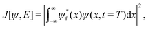
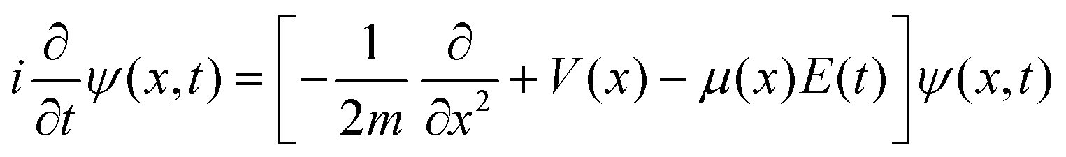
Since the main purpose of this work is to harness reinforcement learning techniques for controlling dynamic chemical systems, we only give a brief overview of quantum optimal control and point the interested reader to several topical reviews in this area.30–33 For chemical systems, the quantum optimal control formalism commences with the time-dependent Schrödinger equation for describing the temporal dynamics of nuclei, which, in atomic units is given by| | 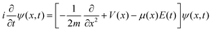 | (1) |
where x is the reduced coordinate along a chosen reaction path, m is the effective mass associated with the molecular motion along the reaction path,34V(x) is the Born–Oppenheimer potential energy function/operator of the molecule, μ(x) is the dipole moment function, E(t) is the time-dependent external electric field, and ψ(x,t) is the wavefunction for the motion of the nuclei along the reduced coordinate path. Both V(x) and μ(x) can be obtained from a quantum chemistry calculation by carrying out a potential energy scan.35–37
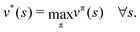
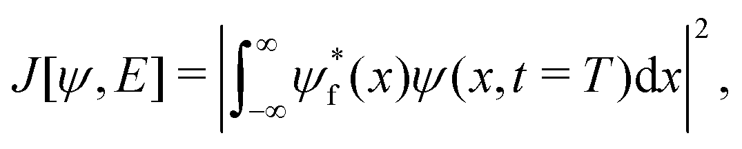
With the time-dependent Schrödinger equation defined in eqn (1), the quantum control problem can be stated as follows: given a starting state ψ0(x) and a desired final state ψf(x), what is the temporal form of the electric field E(t), t ∈ (0,T) that propagates the state ψ0(x) to ψf(x)? In other words, the quantum control formalism seeks the electric field that maximizes the following functional:
| |  | (2) |
where
ψf(
x) is a desired target final wavefunction given by the user, and
ψ(
x,
t =
T) is obtained by propagating
ψ0(
x) in time (
via the time-dependent Schrödinger equation) to
t =
T. In short,
eqn (2) measures the similarity (fidelity) between the target and actual wavefunction at time
T.
In this work, we harness new RL techniques to automatically construct optimal control fields, E(t), that enable desired transitions in these dynamical systems. To test the performance of our RL approach, we compare against the NIC-CAGE (Novel Implementation of Constrained Calculations for Automated Generation of Excitations) code,38 which solves the quantum control problem using a traditional gradient-based approach. Specifically, the NIC-CAGE code utilizes analytic gradients based on a Crank–Nicolson propagator, which are computationally more efficient than other matrix exponential approaches (such as those used in the GRAPE39 or QuTIP40,41 packages) or higher-order time-propagation methods.42 As such, a comparison against the execution times of the already optimized NIC-CAGE code serves as an excellent benchmark test of the performance of our RL methods. Before describing our reinforcement learning approach, we first provide a brief review of Markov decision processes (MDPs) in the next section.
B Review of Markov decision processes (MDPs)
MDPs43 are a class of mathematical formulations for sequential decision-making problems. In an MDP, we define a state space  , an action space
  , a state transition probability P(s′|s,a), and a reward function r(s,a). At each time step t, the state of the “environment” is represented by an element
  . A learning “agent” can interact with this environment by taking some action
  based on st. The environment provides a reward rt+1 = r(st,at) to the agent and transitions to other states st+1 according to the state transition probability function st+1 = P(·|st,at). The above process repeats iteratively. Given the current state st and action at, the state transition function dictates that the next state st+1 is conditionally independent of all previous state and actions.
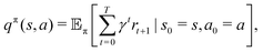
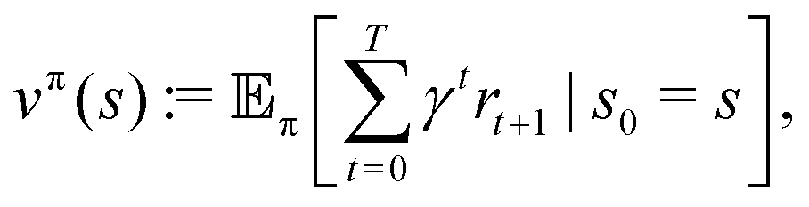
The goal of the learning agent is to find a policy π(a|s), which is a rule for taking actions based on states, such that the expected discounted return vπ(s) is maximized:
| |  | (3) |
| |  | (4) |
The notation

denotes the expectation of the quantity · starting from a state
s, which then follows the policy π thereafter. The constant
γ < 1 controls the contribution of future rewards to the optimizing objective, and
T is the optimization horizon which may be infinite. Note that the policy π(
a|
s) is a probability distribution over

conditioned on an

. The agent takes action by sampling an element from the distribution
at = π(·|
st).
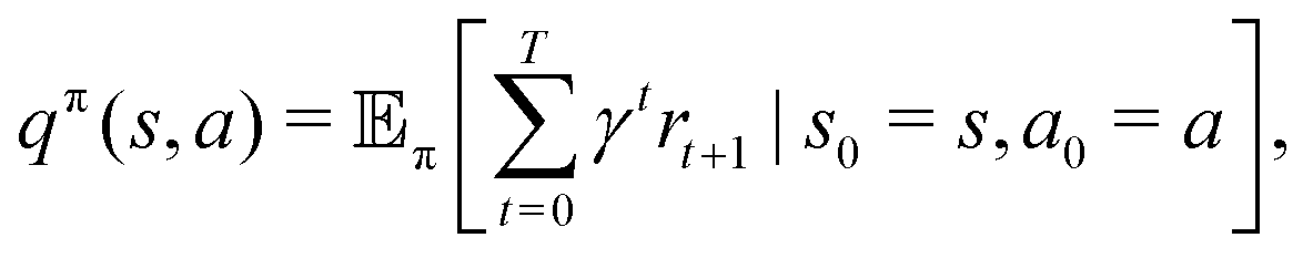
Another function commonly used in reinforcement learning is the action-value function defined as
| |  | (5) |
| |  | (6) |
With these quantities properly defined, we formulate the quantum control problem as an MDP in the next section.
C Formulating quantum control as an MDP
To formulate the quantum control problem as an MDP, we must define the time variable, state, action, and reward:
Time variable.
The time variable, t, of the MDP is naturally defined as the time in the quantum control problem, which we discretize into evenly spaced intervals of duration τ.
State.
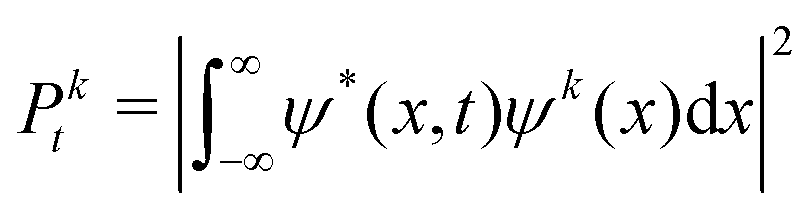
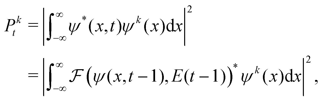
The state at time step t is defined as st = [P0t, P1t, …, PKt, gt]. Pkt, k = 0, …, K is the squared magnitude of the projection of the current wavefunction, ψ(x,t), onto the kth eigenstate, ψk(x), of the time-independent Schrödinger equation:| |  | (7) |
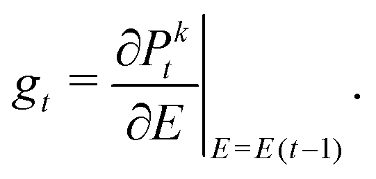
We include the various Pkt terms in our state space since it gives additional information to the reinforcement learning agent about the current wavefunction. The variable K is a design parameter that is described further in Section IV. The variable gt is the gradient of the fidelity with respect to the electric field, E, evaluated at E(t − 1):| | 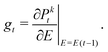 | (8) |
To calculate this gradient, we re-express Pkt as| | 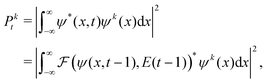 | (9) |
where  is an algorithm that performs one propagation step of the wavefunction (i.e.,
  propagates one step of the time-dependent Schrödinger equation in eqn (1)). We approximate the integral in eqn (9) with a finely-spaced Riemann sum and leverage the auto-differentiation engine from the PyTorch deep learning framework44 to calculate the gradient. Adding this gradient information provides the machine learning agent with the direction in which the fidelity can possibly be improved.
Action.
The action at time step t is defined as the amplitude of the electric field at = E(t), where the minimum and maximum amplitude is restricted to Emin and Emax, respectively.
Reward.
The reward to the agent after taking an action at is defined as rt+1 = Pκt+1 (i.e., the immediate next fidelity score).
This brief explanation completes the formulation of quantum control as a reinforcement learning problem. In the next section, we provide the technical details for utilizing RL to solve our quantum control problem in reduced-dimensional chemical systems.
III Deep reinforcement learning for predicting optimal electric fields
In this section, we describe our DRL approach for solving the MDP problem. An overview of our framework is illustrated in Fig. 1, which shows the MDP formulation, RL algorithm, and the interaction between the two. In the next subsection, we give further details on the theory and algorithms used in our reinforcement learning agent.
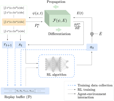 |
| | Fig. 1 RL-based QOC framework utilized in this work. Solid lines represent the interactions between the RL algorithm and the time-dependent Schrödinger equation, blue dashed lines represent the training data collection, and black dashed lines represent the training of the RL algorithm. At each time step t, the RL algorithm outputs an action at based on the state st, and at is then converted to an electric field E(t). The time-dependent Schrödinger equation block performs a forward propagation and a backward differentiation to obtain the next state st+1 and reward rt+1. The tuple st, at, rt+1, and st+1 is stored in the replay buffer  . . | |
A Overview of reinforcement learning
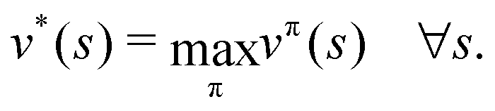
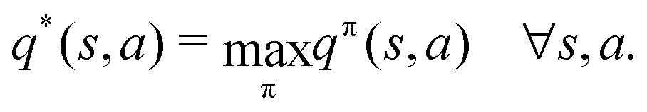
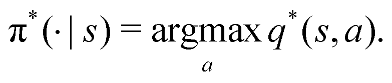
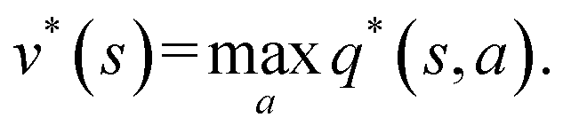
Reinforcement learning (RL) algorithms autonomously estimate the optimal policy π* by interacting with a given environment. It is well-known that under mild technical assumptions, a deterministic stationary optimal policy exists,45 which is given by:| | 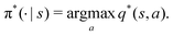 | (10) |
In an optimal policy, the expected discounted return from state s equals v*(s), the optimal state value of s. In other words, 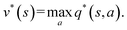 The relationship in eqn (10) reveals that estimating π*(a|s) or q*(s,a), or both at the same time are equally useful in solving MDP problems. As such, RL algorithms can be classified as policy gradient methods (estimating π*), action-value methods (estimating q*), and actor-critic methods (estimating both π* and q*). For MDPs with a finite state and action space, the policy and value functions can be maintained in a table. However, our particular quantum control problem has a continuous state space that must be represented by function approximators such as neural networks.
To learn the optimal policy, RL algorithms must properly balance the conflicting objectives of exploring the state-action space as much as possible to collect environment feedback, while only visiting useful portions to act optimally. This is known as the exploration–exploitation trade-off. In the terminology of quantum control, the RL algorithm must explore different external electric fields, E(t), before it recognizes the optimal one. However, to be efficient, this exploration should not take too long since it may undermine computational performance. We briefly review two of the popular methods to balance exploration and exploitation in our work.
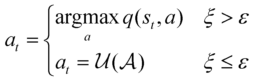
Epsilon greedy.
The Epsilon greedy46 algorithm explores the state-action space by following the optimal policy, while occasionally taking a random action uniformly sampled from the action space:| | 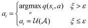 | (11) |
where  is a uniform distribution between 0 and 1, and ε is a constant between 0 and 1. In practice, ε may start with a large value and becomes gradually annealed as the training progresses.
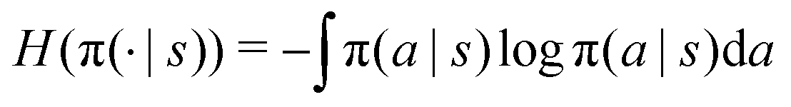
Entropy bonus.
In the maximum entropy RL framework,47 the entropy of the policy 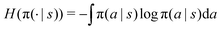 is added to the reward to maintain high stochasticity of the policy when the collected reward value is small:
| | | rh(s,a) = r(s,a) + αH(π(·|s)), | (12) |
where α is the temperature parameter that controls the influence of the entropy to the reward. Policies learned from rh(s,a) tend to have a higher stochasticity than the ones learned from r(s,a) alone. Therefore, the sampled actions at = π(·|s) have a higher chance of visiting a larger portion of the state-action space.
In our work, two DRL algorithms are harnessed to solve the quantum control problem: deep Q learning and soft actor-critic, both of which are described below.
B Deep Q learning
Deep Q learning46 is a value-based algorithm that uses deep neural networks to learn the optimal value function q*(s,a). A neural network qθ(s,a) was used to approximate the optimal value function as follows:| | 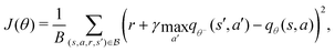 | (13) |
where  is a mini-batch randomly sampled from the experience replay buffer
  . The latter maintains a fixed number of the most recent agent-environment interaction data,
  is the mini-batch size, qθ−(s,a) is another neural network with an identical architecture as qθ, and δ is the learning rate. The parameters θ− are copied from θ after every few iterations to stabilize the training. Since finding the maximum for the Q network over the action space is intractable, the deep Q learning algorithm may only be used for finite and discrete action space MDPs. Discretization is commonly used when the action is continuous, and the epsilon greedy algorithm is typically used in conjunction with deep Q learning. In our MDP formulation of the quantum control problem, the neural network qθ(st,a) is interpreted as the discounted cumulative fidelity score calculated from
  at time t, and the electric field is set to E(t) = a. Therefore, the optimal electric field at time t is
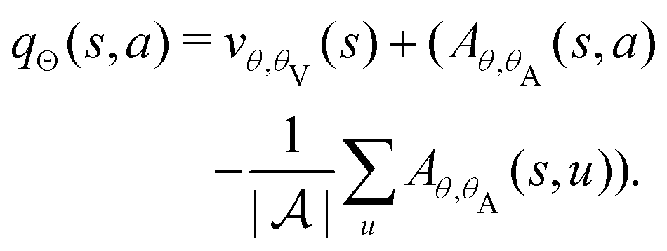
In this paper, we adopt two important extensions to the basic deep Q learning algorithm, namely, the dueling architecture48 and the double deep Q learning,49 which have achieved improved performance on other control benchmarks. The dueling architecture decomposes the Q value estimate into a state value and advantage function estimate according to the formula qπ(s,a) = vπ(s) + Aπ(s,a). As a result, the dueling Q network replaces the output of the standard neural network, qθ(s,a), with two intermediate output streams: vθ,β(s) and Aθ,α(s,a). The final output, which is the Q value estimate, is given by the following aggregation of the two intermediate streams:
| | 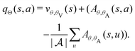 | (15) |
We use the symbol
Θ = (
θ,
θA,
θV) to collectively “absorb” all parameters of the hidden layers and the two output streams. Subtracting the average of
Aθ,α on the right-hand side of
eqn (15) resolves the lack of identifiability of the value-advantage decomposition. The dueling architecture allows the value function to be learned more efficiently.
The double deep Q learning network (DDQN) approach modifies the loss function in eqn (13) as:
| |  | (16) |
Compared with
eqn (13),
eqn (16) decomposes the max operator into a separate action selection and evaluation procedure. This mitigates the overestimation issue with the max operator in
eqn (13) and leads to a more consistent estimation.
C Soft actor-critic
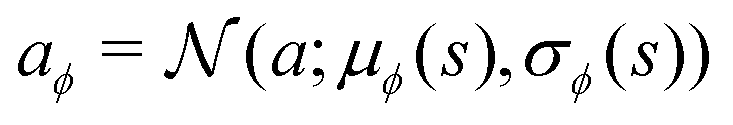
The soft actor-critic (SAC)47 approach is an actor-critic algorithm developed recently using the maximum entropy framework. The algorithm trains deep neural network-parameterized policy and value functions, πϕ(a|s) and qθ(s,a), to approximate the optimal maximum entropy policy and value functions, respectively. πϕ(a|s) is a neural network that takes s as the input and outputs a probability distribution over the action space  . For mathematical tractability purposes, this probability distribution is often chosen as the tanh-squashed Gaussian:
| |  | (17) |
| | | ut = ξt·σϕ(st) + μϕ(st), | (18) |
That is, the neural network outputs the mean μϕ(s) and standard deviation σϕ(s) of the action for a given state s, where the distribution is defined by πϕ(a|s) = tanh(aϕ) and 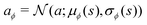 . The tanh function squeezes the Gaussian variable into a finite range and ensures a bounded action. In the context of the quantum control problem, eqn (17)–(19) states that the external electric field, E(t), at time t generated by the SAC algorithm is a Gaussian random variable, whose mean and variance is given by some learned neural network. The variance is maintained to ensure a sufficient exploration of E(t). The action-value function network, qθ(s,a), takes the (s,a) pair as input and outputs a single number to represent the action value.The SAC algorithm additionally employs the target neural network qθ−(s,a), similar to the deep Q learning algorithm. Also, two action-value networks are maintained instead of one to stabilize the training. As a result, four neural networks are responsible for the estimation of the following functions: qθ1(s,a), qθ2(s,a), qθ1−(s,a), and qθ2−(s,a).
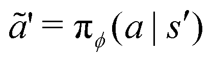
The training of the policy neural network, πϕ(a|s), and value networks, qθi(s,a) for i = 1, 2, are carried out as follows. At each iteration, the policy neural network is trained to minimize the temporal difference error J(θi):
| | 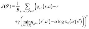 | (20) |
| | | θi ← θi − δ∇J(θi) i = 1, 2, | (21) |
where

is a random sample from the current policy. The policy neural network is trained using the following gradient ascent approach:
| | 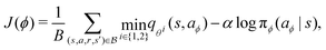 | (22) |
where
aϕ = π
ϕ(
a|
s) is a random sample from the current policy. Finally, the target network is updated using the exponential moving average:
| | | θi− ← ρθi− + (1 − ρ)θi i = 1, 2. | (24) |
D Summary of our RL algorithm for quantum control
Our RL-based quantum control framework is summarized in the Algorithm 1 flowchart. For conciseness, we have summarized the deep Q learning and SAC approaches in the same pseudocode (they differ by Lines 3 and 8). More detailed descriptions of our implementation of these algorithms are given in the ESI.†
|
Algorithm 1 RL for QOC |
| 1: |
Initialize neural network weights and s0 |
| 2: |
for
t = 0,…, do |
| 3: |
Sample at = π(·|st). The sampling is defined by eqn (11) for deep Q learning and eqn (17)–(19) for SAC |
| 4: |
E(t) ← at·Ē |
| 5: |
Perform one environment step to obtain st+1, rt+1 according to Section II A |
| 6: |
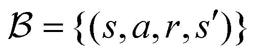
Store (st,at,rt+1,st+1) into the replay buffer  |
| 7: |
Sample mini-batch 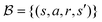 from from  |
| 8: |
Train the RL algorithm by performing eqn (16) for |
|
|
deep Q learning and eqn (20)–(24) for SAC |
| 9: |
ifPκt > ![[P with combining macron]](https://www.rsc.org/images/entities/i_char_0050_0304.gif) then then |
| 10: |
Break |
At each time step t, the agent takes an action, at, according to the state st and converts it to an electric field E(t) = atĒ, where Ē is the upper/lower limit of the magnitude of the electric field. The environment then transitions to the next state according to the Markov decision process defined in Section II C. The agent-environment interaction transition (st,at,rt+1,st+1) is stored in the replay buffer. Tuples of this form will be randomly sampled to train the neural networks of the deep Q learning and SAC algorithm. The procedure stops when the fidelity Ptκ is above a pre-defined threshold , which we set to 0.99 in this work.
IV Results
In this section, we compare the performance of the various RL algorithms against the gradient-based approach from the NIC-CAGE algorithm. Section IV A describes the algorithm and hardware setup used in this work. Section IV B reports the performance of RL compared to the NIC-CAGE benchmarks, and Section IV C concludes with a discussion of a particularly difficult case.
A Numerical setup
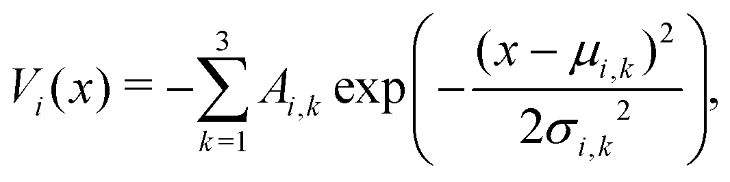
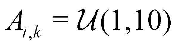
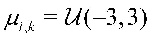
Similar to our previous work on quantum control of molecular systems,23 we generated a set of potentials {Vi(x)}i=1,2,… of the form:| | 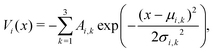 | (25) |
where  ,
,  , and
, and  , and
, and  denotes a uniform distribution. A comprehensive listing of the parameters used to generate the various potentials, Vi(x), in this work can be found in the ESI.† The functional form of these potentials mimic a bond stretching or dissociation process in a photo-induced reaction. The range of x is restricted to the interval [−8,8] and discretized into 192 equally-spaced intervals. The entire time duration T is also discretized into intervals of length 0.1. The range of the electric field amplitude is constrained to lie within the [−0.9,0.9] interval. The total number of states used to define the state space for our RL algorithms is set to 5 (or K = 4 in the notation of Section II). The dipole moment function μ(x) in eqn (1) was set to x.
Algorithm setup.
The hyperparameters for our RL algorithm are provided in Table 1, which we manually tuned on 10 selected potentials. Nevertheless, we found that the algorithm's performance was insensitive to small variations for most of the hyperparameters. Unless specified otherwise, these values were used for all of our subsequent simulations.
Table 1 Hyperparameters used in our RL algorithms
|
|
SAC |
DDQN |
| Hidden layers |
(200, 200) |
(200, 200) |
| Hidden activation |
ReLu |
ReLu |
| Discount factor (γ) |
0.99 |
0.99 |
| Minibatch size |
64 |
64 |
| Optimizer |
Adam |
Adam |
| Learning rate |
0.0003 |
0.0001 |
| Electric field bound (Ē) |
0.2 |
0.1 |
| Temperature parameter (α) |
0.1 |
— |
| Smoothing coefficient (ρ) |
0.005 |
— |
| Target updating frequency |
— |
100 |
| Epsilon max |
— |
0.5 |
| Epsilon min |
— |
0.01 |
| Epsilon annealing |
— |
 of training of training |
| Action discretization |
— |
15 |
Hardware/software setup.
The NIC-CAGE package is implemented in Python with the NumPy and SciPy package; the one-step forward propagation of the Schrödinger equation and the RL algorithms are implemented in Python with the PyTorch deep learning framework. All simulations were executed on the Extreme Science and Engineering Discovery Environment (XSEDE) Comet computing cluster at the University of California, San Diego. To provide a fair comparison between the NIC-CAGE and RL approaches examined in this work, each computation utilized 2 Intel Xeon E5 cores.
B Fidelity and computation time
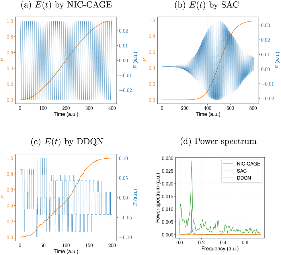
For illustrative purposes, we commence with a relatively easy case for a potential with a small effective mass (m = 1.0) (Fig. 2) to understand the performance of the RL and NIC-CAGE approaches.
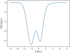 |
| | Fig. 2 Example of a potential with a small effective mass used in this work. | |
The converged electric field and fidelity, as well as the power spectrum of the electric field for all methods are shown in Fig. 3a–c.
 |
| | Fig. 3 Electric fields, E(t), computed by the (a) NIC-CAGE algorithm and various reinforcement learning algorithms: (b) SAC and (c) DDQN. The power spectrum for all cases is shown in panel (d). | |
All of the ML algorithms examined in this work automatically construct an electric field that propagates the initial state to the desired target state with a fidelity larger than 0.99. However, the difference is that the NIC-CAGE algorithm concurrently updates the electric field for all time steps in each iteration, whereas the RL algorithms developed in this paper sequentially add a new electric field data point at each time step (i.e., the RL “learns” the electric field in an automated fashion). Fig. 3d plots the power spectrum for each of the electric fields shown in Fig. 3a–c. Interestingly, the NIC-CAGE and SAC algorithms produce relatively smooth electric fields and power spectra, whereas the DDQN approach employs an action-discretization approach, resulting in an electric field and power spectrum with significant noise. As such, the SAC algorithm can be used to improve other RL methods, such as those used to construct optimal fields for spin-1/2 systems in quantum computing. The control fields obtained in these prior studies are typically not smooth,26 making them difficult to realize in experiments, whereas the SAC algorithm used here can ameliorate these artifacts.
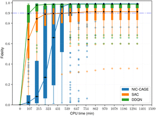
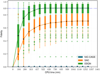
When the effective mass is set to a larger value of m = 10.0, computing the optimal electric field becomes significantly more difficult. Large masses pose significant difficulties since they correspond to quantum optimal control of macroscopic objects (for example, quantum mechanical tunneling through a potential energy barrier is significantly more difficult for a larger mass than a smaller one). For some potentials, the NIC-CAGE algorithm does not converge to a high-fidelity solution within a reasonable computation time. To further compare the performance of the various RL algorithms against the traditional NIC-CAGE approach, we classified all the potentials into three groups based on the range of fidelities obtained by the NIC-CAGE algorithm: [0.75,1.0] designates easy cases, [0.01,0.75) are medium-difficulty cases, and [0.0,0.01) are hard cases. There are 89, 47, and 149 potentials in each group, respectively.
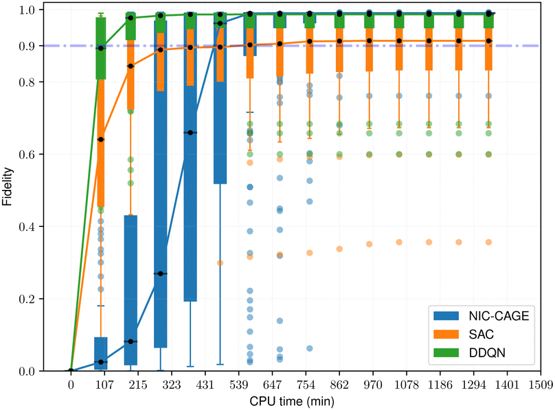
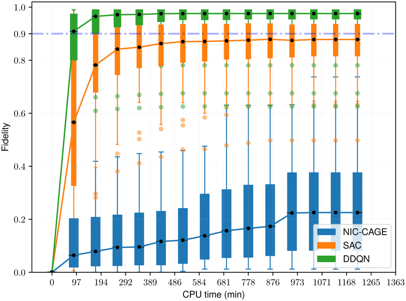
The fidelity vs. computation time for all methods is shown in Fig. 4–6. For the easy cases, the NIC-CAGE benchmark converges to high-fidelity solutions but requires long computation times. In contrast, the DDQN algorithm gives a similar fidelity as the NIC-CAGE benchmarks but with less computational effort. The SAC algorithm is only slightly worse than the DDQN method. Examining the medium-difficulty and hard cases (which account for ∼66% of all the tested potentials), we find that both DDQN and SAC significantly improve on the fidelity compared to the gradient-based NIC-CAGE approach. In particular, both RL methods are significantly more effective in scenarios where the NIC-CAGE algorithm only gives a low-fidelity solution, as shown by the hard cases in Fig. 6. It is worth noting that the quantum control problem for some potentials can be difficult to converge with RL, as shown by the outliers in each of the bar plots. We discuss these special cases in the next subsection and demonstrate that increasing the computation time improves their fidelity for RL (whereas these cases still remain unsolvable with the gradient-based NIC-CAGE algorithm).
 |
| | Fig. 4 Performance comparison between RL and NIC-CAGE on easy cases. | |
 |
| | Fig. 5 Performance comparison between RL and NIC-CAGE on medium-difficulty cases. | |
 |
| | Fig. 6 Performance comparison between RL and NIC-CAGE on hard cases. | |
As shown in Fig. 4–6, DDQN generally produces better results than the SAC method. In the context of machine learning, we carried out an ablation study to show which extension contributes the most to its superior performance. Table 2 shows the fidelity for all cases across Fig. 4–6 arranged in the 10, 50, and 90 percentiles. Each row is a variant of deep Q learning: basic DQN, double DQN, DQN with dueling architecture, and double DQN with dueling architecture. In particular, We found that both extensions improved the performance of DQN, when used alone or combined.
Table 2 Average performance of DQN and its extensions for easy, medium, and hard cases
|
|
Easy |
Medium |
Hard |
All |
| DQN |
0.931 |
0.927 |
0.833 |
0.879 |
| Double DQN |
0.957 |
0.949 |
0.847 |
0.898 |
| Dueling DQN |
0.958 |
0.958 |
0.836 |
0.894 |
| Dueling + double |
0.961 |
0.949 |
0.862 |
0.907 |
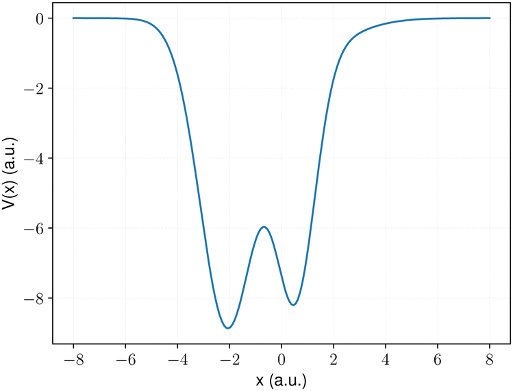
C Case study: double-well potentials and large effective masses
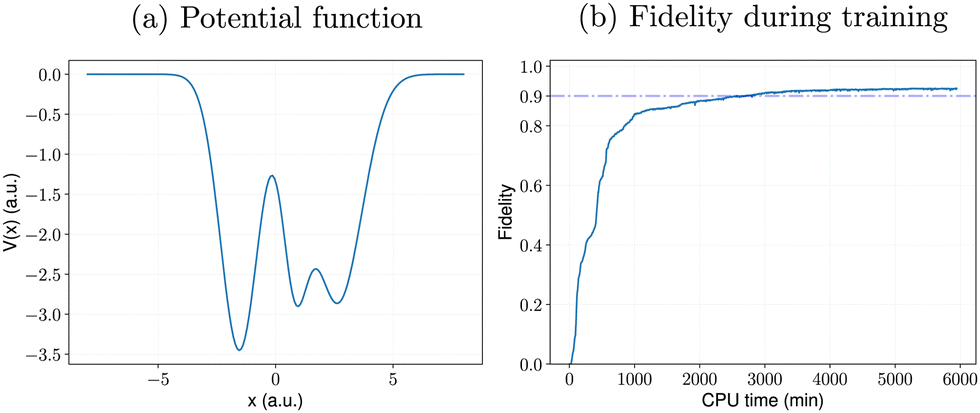
As mentioned in Section IV B, although our RL algorithms generally outperform the gradient-based NIC-CAGE benchmarks, a few outlier potentials can be challenging to converge with RL. One such example is shown in Fig. 7a, which has a complex “double well” shape. These double-well potentials pose significant challenges since they correspond to quantum mechanical tunneling processes through a large potential barrier. The optimal electric fields that enable these unique transitions are typically quite complex. As such, for this potential, the gradient-based NIC-CAGE algorithm dramatically fails to converge (with P < 10−28) even after five hours of computation. However, our DDQN method reaches a much higher fidelity within the same computation time. Most importantly, our DDQN approach eventually reaches a 0.9 fidelity after about 3000 minutes of computation, which is not possible with the NIC-CAGE code. Most importantly, Fig. 7b plots the fidelity during the training, which shows that our RL approach can solve these quantum control problems that are not possible with the gradient-based NIC-CAGE algorithm.
 |
| | Fig. 7 Learning performance of RL for (a) a potential that is difficult to solve with gradient-based quantum control methods. For this particular case, the NIC-CAGE algorithm fails to converge (with a transition probability of P < 10−28) after five hours of computation. In contrast, the DDQN-based reinforcement learning approach gives a higher fidelity and continues to improve as the algorithm runs longer, as shown in panel (b). | |
V Conclusion
In conclusion, we have presented a new reinforcement learning framework for accurately and efficiently solving quantum optimal control problems for dynamical chemical systems. Our approach is formulated as a Markov decision process that leverages RL to autonomously construct electric fields that enable desired transitions in these quantum chemical systems. To test the performance of these techniques, we carried out extensive numerical studies showing that RL produces high fidelity solutions significantly faster than numerically-optimized gradient-based approaches. Regarding the advantages/disadvantages of the RL algorithms explored in this work, DDQN is preferred over SAC if the system under study can accept discrete/non-smooth values of E(t) (the DDQN algorithm is easier to implement and requires less computation per training iteration). However, if discrete values of E(t) are not realizable/acceptable, DDQN cannot be directly implemented, and SAC should be used since it can generate continuous and smooth optimal control fields. Most importantly, we show that both RL approaches can significantly improve the fidelity in quantum control problems that are difficult (or even impossible) to solve with gradient-based methods.
Looking forward, we anticipate that the RL techniques in this work could be used as efficient (and sometimes superior) alternatives to gradient-based approaches in quantum control problems. In particular, our RL approaches are expected to be even more efficient in high-dimensional quantum systems or applications with a large number of qubits. For both of these examples, calculations of the high-dimensional gradients would be computationally expensive, whereas the RL approach (which does not require these gradients) would be significantly more efficient. As such, these new RL techniques could be a viable option for obtaining optimal control fields of large quantum systems where gradient-based calculations are intractable or prohibitively out of reach.
Conflicts of interest
There are no conflicts to declare.
Acknowledgements
This work was supported by the U.S. Department of Energy, Office of Science, Office of Advanced Scientific Computing Research, Scientific Discovery through Advanced Computing (SciDAC) program under Award Number DE-SC0022209. This work used the Extreme Science and Engineering Discovery Environment (XSEDE) Comet computing cluster at the University of California, San Diego, through allocation TG-ENG160024.
References
- D. Castaldo, M. Rosa and S. Corni, Phys. Rev. A, 2021, 103, 022613 CrossRef CAS.
- K. C. Nowack, F. H. L. Koppens, Y. V. Nazarov and L. M. K. Vandersypen, Science, 2007, 318, 1430–1433 CrossRef CAS PubMed.
- M. Kues, C. Reimer, P. Roztocki, L. R. Cortés, S. Sciara, B. Wetzel, Y. Zhang, A. Cino, S. T. Chu, B. E. Little, D. J. Moss, L. Caspani, J. Azaña and R. Morandotti, Nature, 2017, 546, 622–626 CrossRef CAS.
- E. M. Fortunato, M. A. Pravia, N. Boulant, G. Teklemariam, T. F. Havel and D. G. Cory, J. Chem. Phys., 2002, 116, 7599–7606 CrossRef CAS.
- H. J. Williams, L. Caldwell, N. J. Fitch, S. Truppe, J. Rodewald, E. A. Hinds, B. E. Sauer and M. R. Tarbutt, Phys. Rev. Lett., 2018, 120, 163201 CrossRef CAS PubMed.
- A. Bartana, R. Kosloff and D. J. Tannor, Chem. Phys., 2001, 267, 195–207 CrossRef CAS.
- B. L. Brown, A. J. Dicks and I. A. Walmsley, Phys. Rev. Lett., 2006, 96, 173002 CrossRef PubMed.
- M. J. Wright, J. A. Pechkis, J. L. Carini, S. Kallush, R. Kosloff and P. L. Gould, Phys. Rev. A: At., Mol., Opt. Phys., 2007, 75, 051401 CrossRef.
- M. B. Oviedo and B. M. Wong, J. Chem. Theory Comput., 2016, 12, 1862–1871 CrossRef CAS PubMed.
- N. V. Ilawe, M. B. Oviedo and B. M. Wong, J. Chem. Theory Comput., 2017, 13, 3442–3454 CrossRef CAS PubMed.
- N. V. Ilawe, M. B. Oviedo and B. M. Wong, J. Mater. Chem. C, 2018, 6, 5857–5864 RSC.
- M. Maiuri, M. B. Oviedo, J. C. Dean, M. Bishop, B. Kudisch, Z. S. D. Toa, B. M. Wong, S. A. McGill and G. D. Scholes, J. Phys. Chem. Lett., 2018, 9, 5548–5554 CrossRef CAS PubMed.
- B. Kudisch, M. Maiuri, L. Moretti, M. B. Oviedo, L. Wang, D. G. Oblinsky, R. K. Prud'homme, B. M. Wong, S. A. McGill and G. D. Scholes, Proc. Natl. Acad. Sci. U. S. A., 2020, 117, 11289–11298 CrossRef CAS PubMed.
- P. Brumer and M. Shapiro, Acc. Chem. Res., 1989, 22, 407–413 CrossRef CAS.
- J. Somlói, V. A. Kazakov and D. J. Tannor, Chem. Phys., 1993, 172, 85–98 CrossRef.
- W. Zhu, J. Botina and H. Rabitz, J. Chem. Phys., 1998, 108, 1953–1963 CrossRef CAS.
- C. Brif, R. Chakrabarti and H. Rabitz, New J. Phys., 2010, 12, 075008 CrossRef.
- M. Abdelhafez, D. I. Schuster and J. Koch, Phys. Rev. A, 2019, 99, 052327 CrossRef CAS.
-
D. J. Tannor, V. Kazakov and V. Orlov, in Control of Photochemical Branching: Novel Procedures for Finding Optimal Pulses and Global Upper Bounds, ed. J. Broeckhove and L. Lathouwers, Springer US, Boston, MA, 1992, pp. 347–360 Search PubMed.
- N. Khaneja, T. Reiss, C. Kehlet, T. Schulte-Herbrüggen and S. J. Glaser, J. Magn. Reson., 2005, 172, 296–305 CrossRef CAS PubMed.
- T. Caneva, T. Calarco and S. Montangero, Phys. Rev. A: At., Mol., Opt. Phys., 2011, 84, 022326 CrossRef.
- W. Zhu and H. Rabitz, J. Chem. Phys., 1998, 109, 385–391 CrossRef CAS.
- X. Wang, A. Kumar, C. R. Shelton and B. M. Wong, Phys. Chem. Chem. Phys., 2020, 22, 22889–22899 RSC.
- C. Chen, D. Dong, H.-X. Li, J. Chu and T.-J. Tarn, IEEE Trans. Neural Netw. Learn. Syst., 2013, 25, 920–933 Search PubMed.
- T. Fösel, P. Tighineanu, T. Weiss and F. Marquardt, Phys. Rev. X, 2018, 8, 031084 Search PubMed.
- X.-M. Zhang, Z. Wei, R. Asad, X.-C. Yang and X. Wang, Npj Quantum Inf., 2019, 5, 1–7 CrossRef.
- M. Y. Niu, S. Boixo, V. N. Smelyanskiy and H. Neven, Npj Quantum Inf., 2019, 5, 1–8 CrossRef.
- M. Bukov, A. G. Day, D. Sels, P. Weinberg, A. Polkovnikov and P. Mehta, Phys. Rev. X, 2018, 8, 031086 CAS.
- J. Mackeprang, D. B. R. Dasari and J. Wrachtrup, Quantum Mach. Intell., 2020, 2, 1–14 CrossRef.
- P. V. D. Hoff, S. Thallmair, M. Kowalewski, R. Siemering and R. D. Vivie-Riedle, Phys. Chem. Chem. Phys., 2012, 14, 14460–14485 RSC.
- S. Thallmair, D. Keefer, F. Rott and R. de Vivie-Riedle, J. Phys. B: At., Mol. Opt. Phys., 2017, 50, 082001 CrossRef.
- T. Brixner and G. Gerber, ChemPhysChem, 2003, 4, 418–438 CrossRef CAS PubMed.
- M. Dantus and V. V. Lozovoy, Chem. Rev., 2004, 104, 1813–1860 CrossRef CAS PubMed.
-
E. B. Wilson, J. C. Decius and P. C. Cross, Molecular Vibrations: the Theory of Infrared and Raman Vibrational Spectra, Dover Publications, New York, NY, 1955 Search PubMed.
- K. Fukui, Acc. Chem. Res., 1981, 14, 363–368 CrossRef CAS.
- K. Fukui, J. Phys. Chem., 1970, 74, 4161–4163 CrossRef CAS.
- B. M. Wong, A. H. Steeves and R. W. Field, J. Phys. Chem. B, 2006, 110, 18912–18920 CrossRef CAS PubMed.
- A. Raza, C. Hong, X. Wang, A. Kumar, C. R. Shelton and B. M. Wong, Comput. Phys. Commun., 2021, 258, 107541 CrossRef CAS.
- N. Khaneja, T. Reiss, C. Kehlet, T. Schulte-Herbrüggen and S. J. Glaser, J. Magn. Reson., 2005, 172, 296–305 CrossRef CAS PubMed.
- QuTiP: Quantum Toolbox in Python, https://qutip.org/docs/latest/modules/qutip/qobj.html#Qobj.expm.
- J. Johansson, P. Nation and F. Nori, Comput. Phys. Commun., 2013, 184, 1234–1240 CrossRef CAS.
- H. Gharibnejad, B. Schneider, M. Leadingham and H. Schmale, Comput. Phys. Commun., 2020, 252, 106808 CrossRef CAS.
-
R. S. Sutton and A. G. Barto, Reinforcement learning: An introduction, MIT Press, 2018 Search PubMed.
-
A. Paszke, S. Gross, S. Chintala, G. Chanan, E. Yang, Z. DeVito, Z. Lin, A. Desmaison, L. Antiga and A. Lerer, Automatic differentiation in PyTorch, 2017.
-
M. L. Puterman, Markov decision processes: discrete stochastic dynamic programming, John Wiley & Sons, 2014 Search PubMed.
- V. Mnih, K. Kavukcuoglu, D. Silver, A. A. Rusu, J. Veness, M. G. Bellemare, A. Graves, M. Riedmiller, A. K. Fidjeland and G. Ostrovski,
et al.
, Nature, 2015, 518, 529–533 CrossRef PubMed.
-
T. Haarnoja, A. Zhou, P. Abbeel and S. Levine, arXiv, 2018, preprint, arXiv:1801.01290.
-
Z. Wang, T. Schaul, M. Hessel, H. Hasselt, M. Lanctot and N. Freitas, International conference on machine learning, 2016, pp. 1995–2003 Search PubMed.
-
H. Van Hasselt, A. Guez and D. Silver, Proceedings of the AAAI conference on artificial intelligence, 2016 Search PubMed.
|
| This journal is © the Owner Societies 2022 |
Click here to see how this site uses Cookies. View our privacy policy here. 
 a,
Xian
Wang
a,
Xian
Wang
 , an action space
  , a state transition probability P(s′|s,a), and a reward function r(s,a). At each time step t, the state of the “environment” is represented by an element
  . A learning “agent” can interact with this environment by taking some action
  based on st. The environment provides a reward rt+1 = r(st,at) to the agent and transitions to other states st+1 according to the state transition probability function st+1 = P(·|st,at). The above process repeats iteratively. Given the current state st and action at, the state transition function dictates that the next state st+1 is conditionally independent of all previous state and actions.
 denotes the expectation of the quantity · starting from a state s, which then follows the policy π thereafter. The constant γ < 1 controls the contribution of future rewards to the optimizing objective, and T is the optimization horizon which may be infinite. Note that the policy π(a|s) is a probability distribution over
  conditioned on an
  . The agent takes action by sampling an element from the distribution at = π(·|st).
 is an algorithm that performs one propagation step of the wavefunction (i.e.,
  propagates one step of the time-dependent Schrödinger equation in eqn (1)). We approximate the integral in eqn (9) with a finely-spaced Riemann sum and leverage the auto-differentiation engine from the PyTorch deep learning framework44 to calculate the gradient. Adding this gradient information provides the machine learning agent with the direction in which the fidelity can possibly be improved.

 .
.
 The relationship in eqn (10) reveals that estimating π*(a|s) or q*(s,a), or both at the same time are equally useful in solving MDP problems. As such, RL algorithms can be classified as policy gradient methods (estimating π*), action-value methods (estimating q*), and actor-critic methods (estimating both π* and q*). For MDPs with a finite state and action space, the policy and value functions can be maintained in a table. However, our particular quantum control problem has a continuous state space that must be represented by function approximators such as neural networks.
 is a uniform distribution between 0 and 1, and ε is a constant between 0 and 1. In practice, ε may start with a large value and becomes gradually annealed as the training progresses.
 is added to the reward to maintain high stochasticity of the policy when the collected reward value is small:
 is a mini-batch randomly sampled from the experience replay buffer
  . The latter maintains a fixed number of the most recent agent-environment interaction data,
  is the mini-batch size, qθ−(s,a) is another neural network with an identical architecture as qθ, and δ is the learning rate. The parameters θ− are copied from θ after every few iterations to stabilize the training. Since finding the maximum for the Q network over the action space is intractable, the deep Q learning algorithm may only be used for finite and discrete action space MDPs. Discretization is commonly used when the action is continuous, and the epsilon greedy algorithm is typically used in conjunction with deep Q learning. In our MDP formulation of the quantum control problem, the neural network qθ(st,a) is interpreted as the discounted cumulative fidelity score calculated from
  at time t, and the electric field is set to E(t) = a. Therefore, the optimal electric field at time t is

 . For mathematical tractability purposes, this probability distribution is often chosen as the tanh-squashed Gaussian:
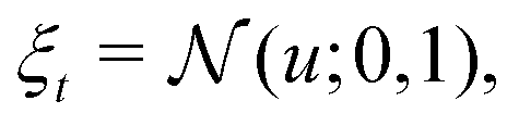
 . The tanh function squeezes the Gaussian variable into a finite range and ensures a bounded action. In the context of the quantum control problem, eqn (17)–(19) states that the external electric field, E(t), at time t generated by the SAC algorithm is a Gaussian random variable, whose mean and variance is given by some learned neural network. The variance is maintained to ensure a sufficient exploration of E(t). The action-value function network, qθ(s,a), takes the (s,a) pair as input and outputs a single number to represent the action value.The SAC algorithm additionally employs the target neural network qθ−(s,a), similar to the deep Q learning algorithm. Also, two action-value networks are maintained instead of one to stabilize the training. As a result, four neural networks are responsible for the estimation of the following functions: qθ1(s,a), qθ2(s,a), qθ1−(s,a), and qθ2−(s,a).

 is a random sample from the current policy. The policy neural network is trained using the following gradient ascent approach:

 from
from 
 ,
,  , and
, and  , and
, and  denotes a uniform distribution. A comprehensive listing of the parameters used to generate the various potentials, Vi(x), in this work can be found in the ESI.† The functional form of these potentials mimic a bond stretching or dissociation process in a photo-induced reaction. The range of x is restricted to the interval [−8,8] and discretized into 192 equally-spaced intervals. The entire time duration T is also discretized into intervals of length 0.1. The range of the electric field amplitude is constrained to lie within the [−0.9,0.9] interval. The total number of states used to define the state space for our RL algorithms is set to 5 (or K = 4 in the notation of Section II). The dipole moment function μ(x) in eqn (1) was set to x.
 of training