 Open Access Article
First-principles NMR of oxide glasses boosted by machine learning†
Thibault
Charpentier

Université Paris-Saclay, CEA, CNRS, NIMBE, 91191 Gif-sur-Yvette cedex, France. E-mail: thibault.charpentier@cea.fr
First published on 26th June 2024
Abstract
Solid-state NMR has established itself as a cutting-edge spectroscopy for elucidating the structure of oxide glasses thanks to several decades of methodological and instrumental progress. First-principles calculations of NMR properties combined with molecular-dynamics (MD) simulations provides a powerful complementary approach for the interpretation of NMR data, although they still suffer from limitations in terms of size, time and high consumption of computational resources. We address this challenge by developing a machine-learning framework to boost predictive modelling of NMR spectra. We use kernel ridge regression techniques (least-squares support vector regression and linear ridge regression) combined with smooth overlap of atomic position (SOAP) atom-centered descriptors to efficiently predict NMR interactions: the isotropic magnetic shielding and the electric field gradient (EFG) tensor. As illustrated in this work, this approach enables the simulation of magic-angle spinning (MAS) and multiple-quantum magic-angle spinning (MQMAS) NMR spectra of very large models (more than 10![[thin space (1/6-em)]](https://www.rsc.org/images/entities/char_2009.gif) 000 atoms) and an efficient averaging of NMR properties over MD trajectories of nanoseconds for incorporating finite-temperature effects, at the computational cost of classical MD simulations. We illustrate these advances for sodium silicate glasses (SiO2–Na2O). NMR parameters (isotropic chemical shift and electric field gradient) could be predicted with an accuracy of 1 to 2% in terms of the total span of the NMR parameter values. To include vibrational effects, an approach is proposed of scaling the EFG tensor in NMR simulations with a factor obtained from the time auto-correlation functions computed on MD trajectories.
000 atoms) and an efficient averaging of NMR properties over MD trajectories of nanoseconds for incorporating finite-temperature effects, at the computational cost of classical MD simulations. We illustrate these advances for sodium silicate glasses (SiO2–Na2O). NMR parameters (isotropic chemical shift and electric field gradient) could be predicted with an accuracy of 1 to 2% in terms of the total span of the NMR parameter values. To include vibrational effects, an approach is proposed of scaling the EFG tensor in NMR simulations with a factor obtained from the time auto-correlation functions computed on MD trajectories.
Introduction
Glasses are ubiquitous materials in modern life because of their low cost but good performances for a high diversity of usages.1–5 Glass indeed offers an infinite combination of compositions (but within a glass formability window) to match the properties of interest. The importance of glass was recognized in 2022 by UNESCO, who declared it as the International Year of Glass.‡ The fundamental challenge in glass science remains the establishment and the knowledge of the relationships between the composition-structure and the properties for the design of new formulations for specific applications. To this aim, molecular dynamics (MD) is the reference technique for building atomistic structural models of glasses and calculating the properties of interest.6–9 Spectroscopic data are, however, needed to assess the MD structural models, which have been mostly provided by neutron and X-ray diffusion experiments for decades.10–12 In this regard and in the context of oxide glasses, NMR remains underexploited and has been generally limited to its ability of providing quantitative information on the structural motifs building the glass network (such as SiO4, AlO4, BO3, and BO4) featuring the so-called short-range order (SRO).NMR has clearly proven over the two last decades to be a key spectroscopy method for deciphering glass structure at various atomic length scale orders (from short to intermediate range order).13–22 Beside the direction of development of advanced radio-frequency pulse sequences for manipulating NMR interactions with an extremely high degree of accuracy,19,21 a second direction was proposed with the introduction of accurate and robust DFT computation methodologies, based on the popular DFT-GIPAW method.23–25 These two directions are of course complementary but both address the essential difficulty encountered in studying amorphous materials such as oxide glasses: the chemical and geometrical disorder introduces broadening of the lines resulting in a strong overlap between NMR peaks, which can persist despite the usage of sophisticated 2D high-resolution techniques. This spectral broadening is engendered by the NMR parameter distribution, a salient feature of glassy materials that cannot be ignored when fitting experimental data.16,26–31 With the help of relationships established either from known crystalline samples or DFT computations, NMR parameter distributions can be inverted to a distribution of a geometrical parameter, such as inter-atomic distances, bond lengths or bond-angle distribution (BAD).31–34 However, such approaches are limited to simple glass compositions and are difficult to extend when there is interplay between several parameters. A direct link between a 3D structural model and the NMR spectrum that can provide such information is therefore necessary.
The continuous increase of computational resources combined with the efficiency and accuracy the DFT-GIPAW method35–37 has enabled its fruitful combination with MD, so that a first-principles NMR approach has emerged as a new tool for investigating glasses.38–41 Within this framework, one can validate the interpretation of experimental data by prediction of NMR fingerprints of atomic species42,43 or assess the quality of MD structural models with a direct comparison with NMR data.44–46 According to our own experience, modern computational resources enable GIPAW-DFT calculations with MD models of up to ∼800 atoms to be performed. DFT inherently limits applicabilities to representative models of glass of several thousands of atoms (a standard size is 5000–10![[thin space (1/6-em)]](https://www.rsc.org/images/entities/char_2009.gif) 000 atoms for MD studies). In addition, investigations of dynamical effects (such as vibrations or diffusion of atoms) on NMR47–50 necessitates long MD trajectories of the order of ns to be considered. Consequently, the recent emergence of machine-learning (ML) methodologies in atomistic modelling51 offers appealing perspectives for accessing larger system sizes and time scales. In solid-state NMR, kernel ridge regression (KRR) techniques were applied to predict NMR shifts in organic molecular solids by Paruzzo et al.52 and in organic molecules by Rupp et al.53 The first application to silicate glasses was provided by Cuny et al.54 using a neural network and by Chaker et al.55 in sodium aluminosilicate glasses with linear ridge regression (LRR). Gaumard et al.56 studied the performances of different kernel regressions in zeolites. Recently, the positions of cesium in clays were refined by Ohkubo et al.57 by using predicted NMR chemical shifts from LRR. In the context of amorphous molecular solids, Cordova et al.58,59 combined MD and KRR-SOAP predicted shifts (ML-Shift),52 to match structural models to experimental MAS NMR spectra. In the context of oxide glasses where quadrupolar nuclei are predominant, prediction of the EFG tensor is needed.
000 atoms for MD studies). In addition, investigations of dynamical effects (such as vibrations or diffusion of atoms) on NMR47–50 necessitates long MD trajectories of the order of ns to be considered. Consequently, the recent emergence of machine-learning (ML) methodologies in atomistic modelling51 offers appealing perspectives for accessing larger system sizes and time scales. In solid-state NMR, kernel ridge regression (KRR) techniques were applied to predict NMR shifts in organic molecular solids by Paruzzo et al.52 and in organic molecules by Rupp et al.53 The first application to silicate glasses was provided by Cuny et al.54 using a neural network and by Chaker et al.55 in sodium aluminosilicate glasses with linear ridge regression (LRR). Gaumard et al.56 studied the performances of different kernel regressions in zeolites. Recently, the positions of cesium in clays were refined by Ohkubo et al.57 by using predicted NMR chemical shifts from LRR. In the context of amorphous molecular solids, Cordova et al.58,59 combined MD and KRR-SOAP predicted shifts (ML-Shift),52 to match structural models to experimental MAS NMR spectra. In the context of oxide glasses where quadrupolar nuclei are predominant, prediction of the EFG tensor is needed.
For atomistic modelling by ML, the so-called atom-centered descriptors (ACDs) play a central role. In the ML context, they were introduced in the seminal work of Behler et al.60 and Bartòk et al.61 The variety of descriptors that have been proposed in the literature is too vast to be covered here (see for, example, ref. 62–64). ACDs must provide a faithful and symmetry-adapted representation of the local environment of a central atom (chemically and geometrically): they must be invariant to translations and permutations, and equivariant to rotations and inversions with regard to the nature of the property of interest. Indeed, for prediction of a scalar property (such as the isotropic magnetic shielding, a charge or an energy), they must be invariant.61 In contrast, for tensorial properties (in our case the electric field gradient (EFG) tensor), they must respect the rotational properties of the second-rank tensors, as was first discussed by Grifasi et al.65 In this work, we have chosen the popular smooth overlap of atomic positions (SOAP) descriptors, which have extensively been studied61,66–69 and shown to have excellent performances for NMR shifts prediction.52,55,56
We present a fully-integrated methodology based on ML kernel tools (linear and kernel ridge regression, least-squares support vector regression, kernel density estimation, and dimensional reduction with incomplete Cholesky decomposition of the kernel Gram matrix) for simulation of the NMR spectra of structural models containing up to several thousands of atoms (calculations were performed on a standard workstation). Our strategy for building a database for ensuring a good transferability of the ML predictions (between various glass compositions and MD temperatures) is presented, as well as ideas for application to the study of the impact of local mobilities (vibrations, or diffusion of atoms) on the NMR spectrum. This opens an appealing perspective for the investigation of ionic conduction in glasses via NMR. Sodium-silicate glasses Si2O–Na2O have been chosen as a representative model of oxide glasses: they contain both I = 1/2 (29Si) and quadrupolar nuclei (23Na and 17O), one with a high local mobility (Na+). Experimental data were taken from previous studies.27,29
Theory and methods
SOAP descriptors for representing the local environment
To represent the local environment of an atom, the SOAP descriptors were chosen.61,66 They are constructed from the expansion of the smoothed atomic density ρi(r) of a central atom i as: | (1) |
![[r with combining circumflex]](https://www.rsc.org/images/entities/i_char_0072_0302.gif) ) are spherical harmonics (
) are spherical harmonics (![[r with combining circumflex]](https://www.rsc.org/images/entities/i_char_0072_0302.gif) = (θ,ϕ) are the polar and azimuthal angles) and Rnl(r) are radial functions. μ is an index that runs on the various atomic species (here, Na, Si and O). In this work, we employ real spherical harmonics (RSH) Ylm(
= (θ,ϕ) are the polar and azimuthal angles) and Rnl(r) are radial functions. μ is an index that runs on the various atomic species (here, Na, Si and O). In this work, we employ real spherical harmonics (RSH) Ylm(![[r with combining circumflex]](https://www.rsc.org/images/entities/i_char_0072_0302.gif) ) and spherical Bessel functions Rnl(r) = jl(αnlr/rcut). αnl is the nth root of the Bessel function jl. This choice ensures that the Rnl(r) form an orthonormal set on the segment [0,rcut] (see Section S4 of the ESI†). With eqn (1), the local environment ρ(r) of the central atom is represented by the set of parameters cμn,l,m. For computations, the expansion of eqn (1) is truncated to values n∈[0,Nmax] and l∈[0,Lmax]. Thus, (rcut, Nmax, Lmax), which are called hyper-parameters, have to be optimized during the training of the ML algorithm. The cμn,l,m are invariant to permutations of the neighbouring atoms and to translations, and they behave like an l-rank tensor under rotations. They represent the local environment of a central atom X in terms of two body interactions. Indeed, for Na2O–SiO2 glasses, the expansion on the index μ yields X–Si, X–O and X–Na terms.
) and spherical Bessel functions Rnl(r) = jl(αnlr/rcut). αnl is the nth root of the Bessel function jl. This choice ensures that the Rnl(r) form an orthonormal set on the segment [0,rcut] (see Section S4 of the ESI†). With eqn (1), the local environment ρ(r) of the central atom is represented by the set of parameters cμn,l,m. For computations, the expansion of eqn (1) is truncated to values n∈[0,Nmax] and l∈[0,Lmax]. Thus, (rcut, Nmax, Lmax), which are called hyper-parameters, have to be optimized during the training of the ML algorithm. The cμn,l,m are invariant to permutations of the neighbouring atoms and to translations, and they behave like an l-rank tensor under rotations. They represent the local environment of a central atom X in terms of two body interactions. Indeed, for Na2O–SiO2 glasses, the expansion on the index μ yields X–Si, X–O and X–Na terms.
For the prediction of the scalar isotropic magnetic shielding value σiso (or equivalently, the isotropic chemical shift), we need rotation-invariant descriptors. The symmetry-adapted descriptors are therefore reduced to cμn,0,0 values, which severely limits the number of descriptors for an environment that can contain around ten atoms (in practice, Nmax ranges from 2 to 12). To overcome this limitation in their seminal work, Bartòk et al.61 introduced the power spectrum, a set of descriptors that combine the cμn,l,m into a sum of rotationally invariant products:
 | (2) |
The power spectrum contains three-body terms, which account for the distribution of angles around the central atom (i.e., Si–X–Si, Si–X–O, Si–X–Na, O–X–O, O–X–Na and Na–O–Na) as was explicitly shown in ref. 67. For tensorial properties of rank λ (i.e., using the familiar notation in NMR, Tλ,m), eqn (2) can be easily generalized to become equivariant:
 | (3) |
Least-squares support vector and linear ridge regression
The kernel ridge regression (KRR) is a generalization of the popular linear ridge regression (LRR) by introducing non-linearities through a kernel function, which can be seen as a measure of the similarity between two environments, here denoted χ. For the isotropic magnetic shielding σiso(χ), the prediction is performed via a linear combination of similarities between the new environment χnew and the training ones χi, as follows: | (4) |
Because of the high dimensionality of the training set, the resolution of the linear system eqn (4) can be cumbersome. The idea of the least-squares support vector regression (LSSVR)71 is to use a reduced set of representative data, denoted ξ, generally referred to as the inducing points or the landmark points. Restricted to this small set, the inversion of the kernel matrix (K + εI)−1 is then tractable. From a NMR perspective, it can be easily understood that many environments in the database are similar (and thus their NMR parameters are also very close), so that fewer points are necessary to support the linear regression eqn (4) (the support vectors). Mathematically, the kernel matrix is then approximated by Kχ,χ ≈ Kχ,ξKξ,ξ−1Kξ,χ with Nξ ≈ 103, whereas Nχ ≈ 105 in our study. This is the Nyström approximation. Resolution of eqn (4) then only requires the diagonalization of Kξ,ξ, as detailed in ref. 71, but the determination of the regression parameters α proceeds so as to account for all samples of the training set. To determine the inducing points ξi from the training set, we found that the incomplete Cholesky decomposition (ICD) of the kernel matrix Kχ,χ (ref. 72) was very efficient and informative, as will be discussed below.
Concerning the EFG tensor, it was predicted in spherical form using the λ-SOAP descriptors, eqn (3), with LRR:
 | (5) |
Note that the summation over l1 and l2 is limited to values such that (λ = 2,m|l1m1l2m2) ≠ 0. In our work with Lmax = 4, from the 25 (l1,l2) pairs, only 16 contribute in eqn (5).
NMR simulations with kernel density estimation
From DFT-GIPAW computations or ML predictions, the NMR parameters x = (δiso,CQ,ηQ) for each atom (here 29Si, 23Na, and 17O) are obtained. A simple approach for simulating the NMR spectrum consists in summing the individual NMR spectra for each atom. This would however be quite ineffective and time-consuming. As was discussed in earlier works,41,73 a better strategy for glasses consists in first reconstructing the NMR parameter distribution. The latter can of course be multi-modal if various species are present; in this case, a clustering algorithm can advantageously help to identify the speciations, an option that is left for future studies. Here a kernel density estimation (KDE)74 approach is adopted for building the NMR parameter distribution p(δiso,CQ,ηQ) on a 3D grid of pre-computed NMR spectra. In the case of silicon-29, quadrupolar parameters can be replaced by CSA values for an accurate modelling, but here a simple 1D approach is adopted so that only p(δiso) is considered (for the reconstruction of anisotropic/isotropic 2D correlation with KDE, see for example ref. 41). In this work, we focus on MQMAS reconstruction of the two quadrupolar nuclei of interest, 17O and 23Na.In the KDE formalism, the value of the distribution is estimated for each grid point xg from the database points xi as:
 | (6) |
From p(xg) and precomputed spectra on the 3D grid, the simulation of the MAS and MQMAS spectra can then be reduced to simple matrix multiplications. In the case of a MQMAS simulation, equations were given in ref. 41. The pre-computed spectra can optionally account for the finite-pulse-width effects (intensity and lineshape distortion) and finite spinning rate. Denoting I(ν;δiso,CQ,ηQ) the precomputed spectra on the grid and neglecting offset effects so that I(ν;δiso,CQ,ηQ) ≈ I(ν − δiso;0,CQ,ηQ), only a 2D grid of (CQ,ηQ) parameters is necessary. Typical grids have the following resolution (boundary values depend on the nucleus): CQ 0.1 MHz, ηQ 0.05, and ν (or equivalently δiso) 0.2 ppm.
This KDE approach underlines that, in the specific case of glasses, the primary goal of the ML prediction is to reconstruct the NMR parameter distribution p(δiso,CQ,ηQ) from the set of environments generated with the MD model(s). Thus, in addition to the quantification of prediction error for each point of the dataset, it is important to compare the reconstructed NMR parameter distribution from predicted ML values (and simulated NMR spectra) with the one computed from the DFT values. Accordingly, many (small) structural models are used to provide a set of sufficiently densely distributed points to estimate p(δiso,CQ,ηQ). The alternative of using larger models offered by ML prediction enables investigation of size effects (such a spurious correlation effect can be induced by the periodic boundary conditions (PBC) in MD simulations).
Optimisation of the hyper-parameters: k-fold cross-validation
Beside the determination of the regression parameters in eqn (4) and (5), the SOAP, kernel and ridge parameters need to be optimized. They are generally referred to as hyper-parameters (with respect to the regression parameters α in eqn (4)). We use a k-fold cross-validation approach which consists in splitting the database into k subsets (in practice, k = 5): the testing set, the validation set and the remainder subsets are in the training set. In LSSVR and LRR, the regression parameters are determined with the training set and the ridge regression parameter is optimized by minimizing the error on the validation set. Note that the inducing points are restricted to being in the training set. The reported error is computed with the testing set. In order to have each point tested, the procedure is repeated k-times by shifting the k-folds. With an initial random shuffling of the database points, the whole procedure can be repeated so that each point can be a testing point more than once, and it provides a robust value of the error standard deviation value. The (hyper-)parameters of the descriptors and kernel width are optimized in an outer loop. Two errors are reported: the mean absolute error (MAE) and root mean square error (RMSE). The latter is sensitive to outliers so that both values are complementary.Design of the NMR database
Structural models of Na2O–SiO2 glasses with % mol Na2O ranging from 10% to 50% (by steps of 10%) were generated with classical MD simulations, as detailed in Sections S1 and S2 of the ESI.† For each composition, 20 independent small models of 300 atoms and 2 supplementary models of 600 atoms were generated for testing the transferability of ML algorithms to larger models when trained on small models. To investigate increased geometrical diversity, structures were extracted at 300 K, 1000 K (both forming the reference set), 1500 K and 2000 K. Long MD trajectories (up to 1 ns) were simulated to study the impact of vibrations on the NMR spectra. Additionally, for each composition, a model of 14![[thin space (1/6-em)]](https://www.rsc.org/images/entities/char_2009.gif) 400 atoms was generated to demonstrate the applicability of machine learning NMR (ml-NMR) simulations to very large systems in short CPU times (here, ∼2 s).
400 atoms was generated to demonstrate the applicability of machine learning NMR (ml-NMR) simulations to very large systems in short CPU times (here, ∼2 s).
Part of the database was recently used for training a machine-learning potential (MLP).76 Two compositions, denoted NS22.5 and NS43.1 (22.5 and 43.1% mol Na2O, respectively) were chosen from this work (∼700 atoms, see Table S2 of the ESI†) for the comparison of the ml-NMR spectra with experimental data (29Si, 23Na and 17O).27 To this end, ab initio MD simulations at 300 K were performed (with CP2K77) for incorporating effects of vibrations at 300 K in the NMR simulations through the computation of correlation functions as detailed below. About 41 structures were extracted every 50 fs to built a NMR database from the first 2ps of the trajectory. In the last 10ps, 8 structures were extracted every 500 fs to check the accuracy of ML prediction.
The NMR properties, the magnetic shielding and electric field gradient tensors, were calculated with the DFT-GIPAW method23 as implemented in VASP (version 5.3.x).35 For referencing the NMR-GIPAW outputs σiso to the isotropic chemical shift values δiso, SiO2 (cristobalite and quartz), Na2SiO3 and α- and β-Na2Si2O5 were used, but in a consistent approach with the MD models: for each system, a supercell of ∼300 atoms was built, its geometry (atomic positions and unit cell parameters) was optimized with CP2K, and the NMR-GIPAW values computed with VASP. Details are given in Section S3 of the ESI.† Notably, the calibration parameters (α and σREF) of the linear regression δiso = −α(σiso − σREF) are given in Table S4 of the ESI.†
Results and discussion
Examination of the NMR database
We propose to examine the diversity of environments in the database by visualizing their respective NMR parameter distribution. For the quadrupolar nuclei, the NMR parameters were efficiently represented with the 2D distribution p(δiso,PQ) using the quadrupolar product PQ2 = CQ2(1 + η2/3). Indeed, PQ (in contrast to CQ and η) is invariant to both the orientation and the ordering principal values of the EFG tensor (VXX,VYY,VZZ). This parameter should therefore be preferred for representing the EFG tensor strength rather than CQ in glasses and during MD trajectories. As shown in Fig. 1, a broadening effect with increasing MD temperature is clearly seen in all data (resulting from a higher geometrical diversity). The aiMD data shows narrower distributions with more pronounced effects of correlation between the NMR parameters for oxygen-17 (note the opposite sign of the linear correlation between NBO and BO). As the MD and aiMD distributions do not overlap, it is therefore expected that MD data cannot predict the aiMD data well. This also points out that, even if less accurate, classical MD produces more disordered structures, and thus is more suitable for building a database with high transferability (a specialized database can be of course generated depending on the aim of the ML prediction). All datasets of the NMR database are given in Table S3 in the ESI.†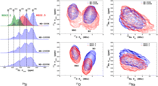 | ||
| Fig. 1 29Si, 17O and 23Na NMR parameter distributions of datasets from the database. MD-xxx (xxx = 300 K, 1000 K, 1500 K and 2000 K) are classical MD models, and NS22.5 and NS43.1 are MLP models extracted from aiMD data at 300 K. For 17O and 23Na, p(δiso,PQ) was calculated using KDE eqn (6). | ||
Learning the isotropic magnetic shielding
For the prediction of σiso (or equivalently δiso), we performed a systematic grid search on the SOAP hyper-parameters as follows: σSOAP in [0.2, 1] Å (step 0.2 Å); rcut = 3, 4, 5 and 6 Å; Nmax from 2 to 12; Lmax was fixed to 4. Details on the computation and optimization of the SOAP descriptors for the MD-300 K and MD-1000 K datasets are given in Sections S4 and S5, respectively, of the ESI.† For each set of (σSOAP,rcut,Nmax) values, the Nyström size (denoted Nξ) was incremented until the MAE had converged (denoted Noptξ). Nξ strongly depends on the variety of environments present in the training set and Noptξ can be therefore considered as a measure of the diversity of the database. An optimal value of σSOAP of 0.4 Å was obtained for all studied nuclei (29Si, 17O and 23Na). Note that no attempt was made to set a different value for each atom. Representative MAE convergence curves are shown in Fig. 2 using MD-300 K as the training set. We observe that increasing the number of radial functions (to better capture the diversity of the environment) effectively requires an increase in Noptξ. The final optimal values that were determined from the dataset MD-300 K + MD-1000 K (the sets used to built the final LSSVR predictors) are given in Table 1 and convergence curves (MAE and RMSE) are shown in Fig. 3. Note that a higher value of Noptξ is necessary with this composite set versus the individual set (for example, Noptξ = 1200 for 17O in MD-300 K and MD-1000 K, see Section S5 of the ESI†) showing the complementarity of the two datasets.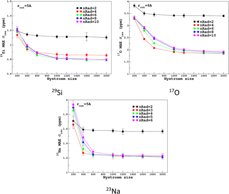 | ||
| Fig. 2 Convergence of σiso MAE with respect to the Nyström size Nξ and the number of radial functions (nRad = Nmax) in the SOAP descriptors for the MD-300 K training set (other SOAP parameters are given in Table 1). | ||
| Atom | σ SOAP (Å) | r cut (Å) | L max | N max | N opt ξ (MD-300 K + 1000 K) | MAE (ppm) | RMSE (ppm) |
|---|---|---|---|---|---|---|---|
| Si | 0.4 | 5 | 4 | 4 | 2000 | 0.93 (0.02) | 1.25 (0.03) |
| Na | 0.4 | 5 | 4 | 6 | 1000 | 1.39 (0.02) | 1.79 (0.03) |
| O | 0.4 | 6 | 4 | 5 | 4000 | 2.25 (0.02) | 3.15 (0.07) |
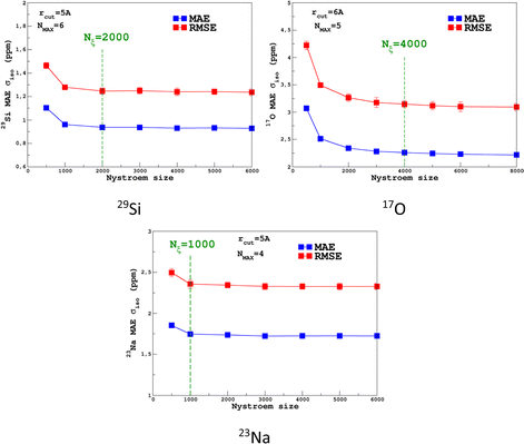 | ||
| Fig. 3 Convergence of the σiso MAE with respect to the Nyström size Nξ for MD-300 K + 1000 K training sets (SOAP parameters are given in Table 1). | ||
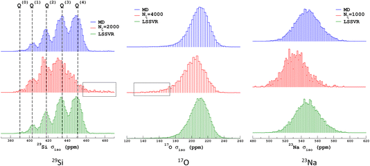
Similarly to Fig. 1, the selection of the inducing points ξ by ICD can be effectively visualized by examination of the NMR parameter distribution, as shown in Fig. 4. We first note the excellent prediction by LSSVR. Interestingly, ICD produces a distribution that differs from the original datasets by enhancing, for example, regions in the tails. Taking as an example the 29Si data, clearly the Q(3) and Q(2) regions are significantly enhanced (which thus suggests a higher local structural diversity) versus the (more regular) Q(4) region. Note that the weak region Q(0) is well-retained by ICD. These results also confirm that the SOAP descriptors combined with a kernel-ICD approach are providing an efficient procedure for extracting the representative set of environments in a database. Attempts to force the selection of inducing points uniformly distributed on σiso did not improve the LSSVR predictions.
Transferability tests between the different training sets were performed and are reported in Section S5 of the ESI.† As expected, high-temperature sets give better accuracy when tested on a lower temperature, compared to the opposite case. Transferability to larger systems (i.e., from 300 to 600 atoms) was also excellent and is illustrated in Fig. 5.
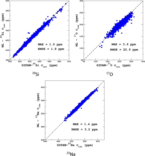 | ||
| Fig. 5 LSSVR versus DFT-GIPAW σiso values for 29Si, 17O and 23Na in the 600-atom MD datasets (300 K + 1000 K). Training was performed on the 300-atom data. | ||
Learning the EFG tensor
It would tempting to use LSSVR to predict the scalar quadrupolar parameters (CQ, η). However, both quantities depend on the ordering of the eigenvalues of the EFG tensor and are therefore discontinuous. Effectively, they are very poorly predicted by LSSVR, as shown in Section S6 of the ESI.† Other ML algorithms (not investigated here) that are robust to discontinuities (such as neural networks or random forests) could be better adapted, but their investigation is out of the scope of the present study. Better LSSVR results are obtained for PQ (which is invariant to rotation), but still show some discrepancies. For these reasons, the option of predicting the full EFG tensor appeared to be the best one.Optimizations of the λ-SOAP descriptors for 23Na and 17O EFG tensors are summarized in Fig. 6. Despite contributions from long-range coulombic interactions, the full EFG tensor is very well captured by the short-range SOAP descriptors (with rcut ≥ 5 Å). As was observed for LSSVR, increasing rcut requires a larger number of radial functions. For the sake of simplicity and efficiency, the values in Table 1 were chosen (so that the SOAP descriptors need only to be computed once for predicting the three NMR parameters). Such good performances of λ-SOAP can be understood as resulting from the correlation that exists between the short- and long-range contributions to the EFG, analogous to the Sternheimer approximation.78 Such correlations were observed in water for quadrupolar nuclei.79 With the MD-300 K + 1000 K datasets, the LRR predictions’ MAEs (RMSEs) for the 17O and 23Na EFG components are 1.6 V Å−2 (2.0 V Å−1) and 0.8 V Å−2 (1.0 V Å−1) respectively, representing ∼1% of their respective total spans. Using the 600-atom MD models (300 K + 1000 K), the same numbers were obtained, showing therefore an excellent transferability, as shown in Fig. 7. 23Na and 17O quadrupolar parameter distributions are very well predicted by LRR λ-SOAP, as shown in Fig. 8.
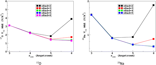 | ||
| Fig. 6 Variations with the cutoff radius of the LRR λ-SOAP mean absolute error (MAE) of the EFG tensor components in the MD-300 K datasets. | ||
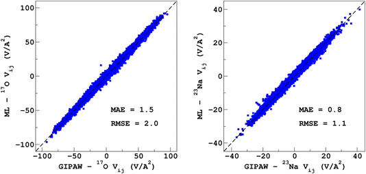 | ||
| Fig. 7 LRR λ-SOAP versus DFT-GIPAW EFG tensor components of the 600-atom MD datasets (300 K + 1000 K). | ||
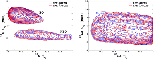 | ||
| Fig. 8 LRR λ-SOAP versus DFT-GIPAW NMR parameter distribution p(CQ,η) for the MD-300 K + 1000 K datasets. | ||
KDE simulation of the MAS and MQMAS NMR spectra
The original motivation for the ML prediction of NMR parameters was to enable the modelling of NMR spectra from structural models of large size (here, 14![[thin space (1/6-em)]](https://www.rsc.org/images/entities/char_2009.gif) 440 atoms) as with modern HPC resources DFT-GIPAW typically addresses 800 atoms with VASP. All subsequent simulations were performed on a standard single processor (Intel CORE i7). Calculations for the large models took around 2 seconds; the most time-consuming part was the calculation of the SOAP descriptors (see Fig. S5 in the ESI†). 23Na and 17O MAS NMR spectra (for the latter we show the isotropic projections of the MQMAS spectrum) are shown in Fig. 9 (MQMAS spectra are given in Sections S8 and S9 of the ESI†).
440 atoms) as with modern HPC resources DFT-GIPAW typically addresses 800 atoms with VASP. All subsequent simulations were performed on a standard single processor (Intel CORE i7). Calculations for the large models took around 2 seconds; the most time-consuming part was the calculation of the SOAP descriptors (see Fig. S5 in the ESI†). 23Na and 17O MAS NMR spectra (for the latter we show the isotropic projections of the MQMAS spectrum) are shown in Fig. 9 (MQMAS spectra are given in Sections S8 and S9 of the ESI†).
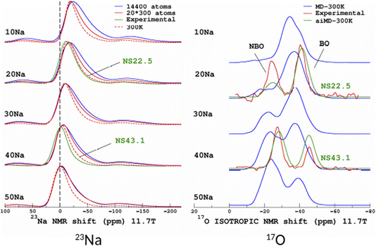 | ||
| Fig. 9 ML simulations of 23Na (left) and 17O (right) MAS and isotropic (isotropic projection of the MQMAS spectra) NMR spectra of the SiO2–Na2O glasses from 10% to 50% mol. Na2O (denoted 10Na to 50Na). For the purpose of comparison, experimental data from ref. 27 are shown (22.5% and 43.1% mol. Na2O, denoted NS22.5 and NS43.1, respectively). For 17O, ML simulations from aiMD structural models (aiMD-300 K) are also shown. | ||
Focusing first on the 23Na NMR data and classical MD models, we observe a discrepancy between the large- and small-model spectra. This is indicative of the effect of the PBC on the structure of the small models, but without impacting the transferability of the ML predictors (Fig. 5 and 7). The comparison with experimental data shows a good agreement, except for the width of the spectra, which is due to an overestimated mean value of the quadrupolar coupling constant, as already observed.29 As will be shown below, accounting for short-time-scale averaging by vibrations significantly reduces the discrepancies. Considering the 17O NMR data, we note a strong deviation of the classical MD NMR model spectra from the experimental data. This is due to the approximate Si–O and Si–O–Si bond angle values predicted in classical MD, in contrast to aiMD (DFT) data, which yields an excellent agreement in the position of the NBO and BO peaks (intensities differ because the impact of the MQMAS pulse sequence was not taken into account for the sake of simplicity). Those simulated spectra can be useful for many purposes. One of them is the assessment of analytical models of NMR parameter distributions, such as the Gaussian Isotropic Model80,81 (GIM) for fitting the 23Na NMR data, for example.
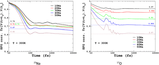
To quantify the impact of atomic vibrations on the NMR parameters, we investigated the auto-correlation functions of the two NMR interactions of interest in this work, Gδ(τ) = 〈δ(τ + t0)δ(t0)〉t0 and GEFG(τ) = 〈V(τ + t0)V(t0)〉t0, calculated on MD trajectories at 300 K. 〈〉t0 denotes the ensemble average that includes here the averaging over all initial times t0 and over all atoms. At short-time scales, Gδ(τ) is a constant function (∼1) at 300 K, thus meaning a very minimal impact of vibrations. In contrast, GEFG(τ) is decaying on the typical time-scale of vibrations (10–100 fs), with a stronger effect for 23Na in contrast to 17O, as illustrated in Fig. 10. After that first decay, the EFG time-correlation function reaches a plateau that can be considered, in a first approximation, as the time-averaged EFG that really contributes to the NMR spectra (whereas the initial decaying part controls the relaxation times,50 but this will be not discussed here). Using the plateauing value as a scaling factor of the frozen EFG tensors (we assume an isotropic scaling), vibrations can then be simply incorporated into the NMR spectra, as shown for 23Na (left panel in Fig. 10, dashed lines). This clearly improves the simulations (see especially 20Na). We note that for 40Na, the experimental width is still overestimated. Indeed, a longer time-scale would be needed to account for the diffusion of Na atoms at 300 K (Na-rich glasses show a higher Na mobility82). The time-scale of the MD simulations is still well below the typical Larmor period for 23Na (here ∼8 ns at 11.7 T). Interestingly, aiMD simulations gave very close curves for the EFG correlation functions, as shown in Section S10 of the ESI.† This means that classical MD potentials are able to capture the vibrational averaging with a good accuracy.
Conclusion
We have described in this paper new computational methodologies for modelling NMR spectra of oxide glasses, combining prediction of NMR properties by ML kernel methods with efficient simulations using KDE of the NMR parameter distribution. We have shown that the SOAP descriptors are very efficient and symmetry-adapted for representing the local environment in the prediction of NMR interactions, be it a scalar (isotropic magnetic shielding value) or a matrix (the EFG second-rank symmetric tensor). Our strategy to build an NMR database that embraces a sufficiently large variety of environments (in terms of both geometrical and chemical disorder) was based on MD simulations at various temperatures and for various glass compositions. It was shown that small models were suitable to build ML predictors that are transferable to much larger systems (here, more than 10![[thin space (1/6-em)]](https://www.rsc.org/images/entities/char_2009.gif) 000 atoms). Most representative environments could be extracted with incomplete Cholesky decomposition of the kernel Gram matrix of the dataset, providing an efficient tool for analysis of the database, as confirmed by the examination of the NMR parameter distributions. Appealing perspectives for an easy incorporation of finite-temperature effects (vibrations) in NMR simulations were presented. Because of its fundamental importance in glass science, ml-NMR will clearly enable NMR investigations of melts (with high-temperature NMR20) to be now more closely connected to MD simulations by computation of the underlying correlation functions of NMR observations. The next step is the incorporation of NMR spectra as direct constraints in the reconstruction of the 3D glass structure of glasses, in the Reverse Monte-Carlo simulations widely used in glass science.11,12,83
000 atoms). Most representative environments could be extracted with incomplete Cholesky decomposition of the kernel Gram matrix of the dataset, providing an efficient tool for analysis of the database, as confirmed by the examination of the NMR parameter distributions. Appealing perspectives for an easy incorporation of finite-temperature effects (vibrations) in NMR simulations were presented. Because of its fundamental importance in glass science, ml-NMR will clearly enable NMR investigations of melts (with high-temperature NMR20) to be now more closely connected to MD simulations by computation of the underlying correlation functions of NMR observations. The next step is the incorporation of NMR spectra as direct constraints in the reconstruction of the 3D glass structure of glasses, in the Reverse Monte-Carlo simulations widely used in glass science.11,12,83
Data availability
The data that support the findings of this study (DFT-GIPAW data for structures of the NMR database) are available at https://doi.org/10.5281/zenodo.12314395.Conflicts of interest
There are no conflicts to declare.Acknowledgements
This work was granted access to the HPC resources of TGCC under the allocation DARI-A0110906303, DARI-A0130906303, and DARI-A0150906303 attributed by GENCI (Grand Equipement National de Calcul Intensif).Notes and references
- R. E. Youngman, in 22 Silicate Glasses and Their Impact on Humanity, De Gruyter, 2022, pp. 1015–1038, DOI:10.1515/9781501510939-023.
- J. C. Mauro, C. S. Philip, D. J. Vaughn and M. S. Pambianchi, Glass science in the United States: current status and future directions, Int. J. Appl. Glass Sci., 2014, 5(1), 2–15, DOI:10.1111/ijag.12058.
- L. Li, H. Lin and S. Qiao, et al., Integrated flexible chalcogenide glass photonic devices, Nat. Photonics, 2014, 8(8), 643–649, DOI:10.1038/nphoton.2014.138.
- S. Gin, A. Abdelouas and L. J. Criscenti, et al., An international initiative on long-term behavior of high-level nuclear waste glass, Mater. Today, 2013, 16(6), 243–248, DOI:10.1016/j.mattod.2013.06.008.
- A. K. Varshneya and J. C. Mauro, Fundamentals of Inorganic Glasses, Elsevier, 3 edn, 2019 Search PubMed.
- H. Liu, Z. Zhao and Q. Zhou, et al., Challenges and opportunities in atomistic simulations of glasses: a review, C. R. Géosci., 2022, 354(S1), 35–77, DOI:10.5802/crgeos.116.
- A. Takada, Atomistic simulations of glass structure and properties, in Encyclopedia of Glass Science, Technology, History, and Culture, ed. P. Richet, R. Conradt, A. Takada and J. Dyon, Wiley, 1st edn, 2021, pp. 221–232, DOI:10.1002/9781118801017.ch2.8.
- J. Du, Molecular dynamics simulations of oxide glasses, in Springer Handbook of Glass, ed. J. D. Musgraves, J. Hu and L. Calvez, Springer International Publishing, Cham, 2019, pp. 1131–1155, DOI:10.1007/978-3-319-93728-1_32.
- J. Du and A. N. Cormack, Atomistic Simulations of Glasses: Fundamentals and Applications – ICG|International Commission on Glass, 2022 Search PubMed.
- A. C. Hannon, Neutron diffraction techniques for structural studies of glasses, in Modern Glass Characterization, John Wiley & Sons, Ltd, 2015, pp. 1–83, DOI:10.1002/9781119051862.ch5.
- G. Evrard and L. Pusztai, Reverse monte carlo modelling of the structure of disordered materials with RMC++: a new implementation of the algorithm in C++, J. Phys.: Condens. Matter, 2005, 17(5), S1, DOI:10.1088/0953-8984/17/5/001.
- R. L. McGreevy, Reverse monte carlo modelling, J. Phys.: Condens. Matter, 2001, 13(46), R877, DOI:10.1088/0953-8984/13/46/201.
- M. Edén, Chapter Four – 27Al NMR studies of aluminosilicate glasses, in Annual Reports on NMR Spectroscopy, ed. G. A. Webb, Academic Press 2015, vol. 86,, pp. 237–331 Search PubMed.
- M. Edén, NMR studies of oxide-based glasses, Annu. Rep. Sect. C: Phys. Chem., 2012, 108(1), 177–221, 10.1039/C2PC90006H.
- D. Massiot, R. J. Messinger and S. Cadars, et al., Topological, geometric, and chemical order in materials: insights from solid-state NMR, Acc. Chem. Res., 2013, 46(9), 1975–1984, DOI:10.1021/ar3003255.
- M. Edén, Probing oxide-based glass structures by solid-state NMR: opportunities and limitations, J. Magn. Reson. Open, 2023, 16–17, 100112, DOI:10.1016/j.jmro.2023.100112.
- K. J. D. MacKenzie and M. E. Smith, Multinuclear Solid-State Nuclear Magnetic Resonance of Inorganic Materials, Pergamon, 1st edn, 2002, vol. 6 Search PubMed.
- H. Eckert, Structural characterization of noncrystalline solids and glasses using solid state NMR, Prog. Nucl. Magn. Reson. Spectrosc., 1992, 24(3), 159–293, DOI:10.1016/0079-6565(92)80001-V.
- M. Deschamps, F. Fayon, V. Montouillout and D. Massiot, Through-bond homonuclear correlation experiments in solid-state NMR applied to quadrupolar nuclei in Al–O–P–O–Al chains, Chem. Commun., 2006, 1924–1925, 10.1039/B600514D.
- D. Massiot, F. Fayon and V. Montouillout, et al., Structure and dynamics of oxide melts and glasses: a view from multinuclear and high temperature NMR, J. Non-Cryst. Solids, 2008, 354(2–9), 249–254, DOI:10.1016/j.jnoncrysol.2007.06.097.
- M. Deschamps, F. Fayon and J. Hiet, et al., Spin-counting NMR experiments for the spectral editing of structural motifs in solids, Phys. Chem. Chem. Phys., 2008, 10(9), 1298–1303, 10.1039/B716319C.
- H. Eckert, Advanced dipolar solid state NMR spectroscopy of glasses, in Modern Glass Characterization, John Wiley & Sons, Ltd, 2015, pp. 1–46, DOI:10.1002/9781119051862.ch9.
- C. J. Pickard and F. Mauri, All-electron magnetic response with pseudopotentials: NMR chemical shifts, Phys. Rev. B: Condens. Matter Mater. Phys., 2001, 63(24), 245101, DOI:10.1103/PhysRevB.63.245101.
- T. Charpentier, The PAW/GIPAW approach for computing NMR parameters: a new dimension added to NMR study of solids, Solid State Nucl. Magn. Reson., 2011, 40(1), 1–20, DOI:10.1016/j.ssnmr.2011.04.006.
- C. Bonhomme, C. Gervais and F. Babonneau, et al., First-principles calculation of NMR parameters using the gauge including projector augmented wave method: a chemist’s point of view, Chem. Rev., 2012, 112(11), 5733–5779, DOI:10.1021/cr300108a.
- D. Massiot, F. Fayon and M. Capron, et al., Modelling one- and two-dimensional solid-state NMR spectra, Magn. Reson. Chem., 2002, 40(1), 70–76, DOI:10.1002/mrc.984.
- F. Angeli, O. Villain, S. Schuller, S. Ispas and T. Charpentier, Insight into sodium silicate glass structural organization by multinuclear NMR combined with first-principles calculations, Geochim. Cosmochim. Acta, 2011, 75(9), 2453–2469, DOI:10.1016/j.gca.2011.02.003.
- E. Gambuzzi, A. Pedone, M. C. Menziani, F. Angeli, P. Florian and T. Charpentier, Calcium environment in silicate and aluminosilicate glasses probed by 43Ca MQMAS NMR experiments and MD-GIPAW calculations, Solid State Nucl. Magn. Reson., 2015, 68–69, 31–36, DOI:10.1016/j.ssnmr.2015.04.003.
- E. Gambuzzi, T. Charpentier, M. C. Menziani and A. Pedone, Computational interpretation of 23 Na MQMAS NMR spectra: a comprehensive investigation of the Na environment in silicate glasses, Chem. Phys. Lett., 2014, 612, 56–61, DOI:10.1016/j.cplett.2014.08.004.
- F. Angeli, M. Gaillard, P. Jollivet and T. Charpentier, Contribution of 43Ca MAS NMR for probing the structural configuration of calcium in glass, Chem. Phys. Lett., 2007, 440(4–6), 324–328, DOI:10.1016/j.cplett.2007.04.036.
- F. Angeli, O. Villain and S. Schuller, et al., Effect of temperature and thermal history on borosilicate glass structure, Phys. Rev. B: Condens. Matter Mater. Phys., 2012, 85(5), 054110, DOI:10.1103/PhysRevB.85.054110.
- T. M. Clark, P. J. Grandinetti, P. Florian and J. F. Stebbins, Correlated structural distributions in silica glass, Phys. Rev. B: Condens. Matter Mater. Phys., 2004, 70(6), 064202, DOI:10.1103/PhysRevB.70.064202.
- T. Charpentier, P. Kroll and F. Mauri, First-principles nuclear magnetic resonance structural analysis of vitreous silica, J. Phys. Chem. C, 2009, 113(18), 7917–7929, DOI:10.1021/jp900297r.
- F. Angeli, T. Charpentier, P. Faucon and J.-C. Petit, Structural characterization of glass from the inversion of 23Na and 27Al 3Q-MAS NMR spectra, J. Phys. Chem. B, 1999, 103(47), 10356–10364, DOI:10.1021/jp9910035.
- F. Vasconcelos, G. A. de Wijs, R. W. A. Havenith, M. Marsman and G. Kresse, Finite-field implementation of NMR chemical shieldings for molecules: direct and converse gauge-including projector-augmented-wave methods, J. Chem. Phys., 2013, 139(1), 014109, DOI:10.1063/1.4810799.
- C. J. Pickard and F. Mauri, Nonlocal pseudopotentials and magnetic fields, Phys. Rev. Lett., 2003, 91(19), 196401, DOI:10.1103/PhysRevLett.91.196401.
- S. A. Joyce, J. R. Yates, C. J. Pickard and F. Mauri, A first principles theory of nuclear magnetic resonance J-coupling in solid-state systems, J. Chem. Phys., 2007, 127(20), 204107, DOI:10.1063/1.2801984.
- T. Charpentier, S. Ispas, M. Profeta, F. Mauri and C. J. Pickard, First-principles calculation of 17O, 29Si, and 23Na NMR spectra of sodium silicate crystals and glasses, J. Phys. Chem. B, 2004, 108(13), 4147–4161, DOI:10.1021/jp0367225.
- T. Charpentier, M. C. Menziani and A. Pedone, Computational simulations of solid state NMR spectra: a new era in structure determination of oxide glasses, RSC Adv., 2013, 3(27), 10550–10578, 10.1039/C3RA40627J.
- A. Pedone, Recent advances in solid-state NMR computational spectroscopy: the case of alumino-silicate glasses, Int. J. Quantum Chem., 2016, 116, 1520–1531, DOI:10.1002/qua.25134.
- A. Pedone, T. Charpentier and M. C. Menziani, Multinuclear NMR of CaSiO3 glass: simulation from first-principles, Phys. Chem. Chem. Phys., 2010, 12(23), 6054, 10.1039/b924489a.
- A. Pedone, T. Charpentier, G. Malavasi and M. C. Menziani, New insights into the atomic structure of 45S5 bioglass by means of solid-state NMR spectroscopy and accurate first-principles simulations, Chem. Mater., 2010, 22(19), 5644–5652, DOI:10.1021/cm102089c.
- S. Chakraborty, D. C. Bobela, P. C. Taylor and D. A. Drabold, Voids in hydrogenated amorphous silicon: a comparison of ab initio simulations and proton NMR studies, MRS Proc., 2008, 1066, 10661102, DOI:10.1557/PROC-1066-A11-02.
- M. Bertani, N. Bisbrouck, J.-M. Delaye, F. Angeli, A. Pedone and T. Charpentier, Effects of magnesium on the structure of aluminoborosilicate glasses: NMR assessment of interatomic potentials models for molecular dynamics, J. Am. Ceram. Soc., 2023, 106(9), 5501–5521, DOI:10.1111/jace.19157.
- Y. Ishii, M. Salanne, T. Charpentier, K. Shiraki, K. Kasahara and N. Ohtori, A DFT-based aspherical ion model for sodium aluminosilicate glasses and melts, J. Phys. Chem. C, 2016, 120(42), 24370–24381, DOI:10.1021/acs.jpcc.6b08052.
- A. F. Harper, S. P. Emge, P. C. M. M. Magusin, C. P. Grey and A. J. Morris, Modelling amorphous materials via a joint solid-state NMR and X-ray absorption spectroscopy and DFT approach: application to alumina, Chem. Sci., 2023, 14(5), 1155–1167, 10.1039/D2SC04035B.
- J.-N. Dumez and C. J. Pickard, Calculation of NMR chemical shifts in organic solids: accounting for motional effects, J. Chem. Phys., 2009, 130(10), 104701, DOI:10.1063/1.3081630.
- J. Schmidt, J. Hutter, H.-W. Spiess and D. Sebastiani, Beyond isotropic tumbling models: nuclear spin relaxation in liquids from first principles, ChemPhysChem, 2008, 9(16), 2313–2316, DOI:10.1002/cphc.200800435.
- S. Sen and T. Mukerji, A molecular dynamics simulation study of ionic diffusion and NMR spin-lattice relaxation in Li2Si4O9 glass, J. Non-Cryst. Solids, 2001, 293–295, 268–278, DOI:10.1016/S0022-3093(01)00679-2.
- S. Badu, L. Truflandier and J. Autschbach, Quadrupolar NMR spin relaxation calculated using ab initio molecular dynamics: group 1 and group 17 ions in aqueous solution, J. Chem. Theory Comput., 2013, 9(9), 4074–4086, DOI:10.1021/ct400419s.
- Machine Learning Meets Quantum Physics, ed. K. T. Schütt, S. Chmiela, O. A. Von Lilienfeld, A. Tkatchenko, K. Tsuda and K.-R. Müller, Springer International Publishing, Cham, 2020, DOI:10.1007/978-3-030-40245-7.
- F. M. Paruzzo, A. Hofstetter, F. Musil, S. De, M. Ceriotti and L. Emsley, Chemical Shifts in Molecular Solids by Machine Learning, Nat. Commun., 2018, 9, 4501 CrossRef PubMed.
- M. Rupp, R. Ramakrishnan and O. A. von Lilienfeld, Machine learning for quantum mechanical properties of atoms in molecules, J. Phys. Chem. Lett., 2015, 6(16), 3309–3313, DOI:10.1021/acs.jpclett.5b01456.
- J. Cuny, Y. Xie, C. J. Pickard and A. A. Hassanali, Ab initio quality NMR parameters in solid-state materials using a high-dimensional neural-network representation, J. Chem. Theory Comput., 2016, 12, 765–773, DOI:10.1021/acs.jctc.5b01006.
- Z. Chaker, M. Salanne, J.-M. Delaye and T. Charpentier, NMR shifts in aluminosilicate glasses via machine learning, Phys. Chem. Chem. Phys., 2019, 21, 21709–21725, 10.1039/C9CP02803J.
- R. Gaumard, D. Dragún and J. N. Pedroza-Montero, et al., Regressionmachine learning models used to predict DFT-computed NMR parameters of zeolites, Computation, 2022, 10(5), 74, DOI:10.3390/computation10050074.
- T. Ohkubo, A. Takei and Y. Tachi, et al., New approach to understanding the experimental 133Cs NMR chemical shift of clay minerals via machine learning and DFT-GIPAW calculations, J. Phys. Chem. A, 2023, 127(4), 973–986, DOI:10.1021/acs.jpca.2c08880.
- M. Cordova, M. Balodis and A. Hofstetter, et al., Structure determination of an amorphous drug through large-scale NMR predictions, Nat. Commun., 2021, 12(1), 2964, DOI:10.1038/s41467-021-23208-7.
- M. Cordova, P. Moutzouri and S. O. Nilsson Lill, et al., Atomic-level structure determination of amorphous molecular solids by NMR, Nat. Commun., 2023, 14(1), 5138, DOI:10.1038/s41467-023-40853-2.
- J. Behler and M. Parrinello, Generalized neural-network representation of high-dimensional potential-energy surfaces, Phys. Rev. Lett., 2007, 98(14), 146401, DOI:10.1103/PhysRevLett.98.146401.
- A. P. Bartók, R. Kondor and G. Csányi, On representing chemical environments, Phys. Rev. B: Condens. Matter Mater. Phys., 2013, 87(18), 184115, DOI:10.1103/PhysRevB.87.184115.
- J. Schmidt, M. R. G. Marques, S. Botti and M. A. L. Marques, Recent advances and applications of machine learning in solid-state materials science, NPJ Comput. Mater., 2019, 5, 83, DOI:10.1038/s41524-019-0221-0.
- M. F. Langer, A. Goeßmann and M. Rupp, Representations of molecules and materials for interpolation of quantum-mechanical simulations via machine learning, NPJ Comput. Mater., 2022, 8, 41, DOI:10.1038/s41524-022-00721-x.
- V. L. Deringer, N. Bernstein and A. P. Bartók, et al., Realistic atomistic structure of amorphous silicon from machine-learning-driven molecular dynamics, J. Phys. Chem. Lett., 2018, 9(11), 2879–2885, DOI:10.1021/acs.jpclett.8b00902.
- A. Grisafi, D. M. Wilkins, G. Csányi and M. Ceriotti, Symmetry-adapted machine learning for tensorial properties of atomistic systems, Phys. Rev. Lett., 2018, 120(3), 036002, DOI:10.1103/PhysRevLett.120.036002.
- E. Kocer, J. K. Mason and H. Erturk, Continuous and optimally complete description of chemical environments using spherical bessel descriptors, AIP Adv., 2020, 10(1), 015021, DOI:10.1063/1.5111045.
- R. Jinnouchi, F. Karsai and G. Kresse, On-the-fly machine learning force field generation: application to melting points, Phys. Rev. B, 2019, 100(1), 014105, DOI:10.1103/PhysRevB.100.014105.
- R. Jinnouchi, F. Karsai, C. Verdi, R. Asahi and G. Kresse, Descriptors representing two- and three-body atomic distributions and their effects on the accuracy of machine-learned inter-atomic potentials, J. Chem. Phys., 2020, 152(23), 234102, DOI:10.1063/5.0009491.
- M. J. Willatt, F. Musil and M. Ceriotti, Atom-density representations for machine learning, J. Chem. Phys., 2019, 150(15), 154110, DOI:10.1063/1.5090481.
- C. E. Rasmussen and C. K. I. Williams, Gaussian Processes for Machine Learning, The MIT Press, 2005, DOI:10.7551/mitpress/3206.001.0001.
- K. De Brabanter, J. De Brabanter, J. A. K. Suykens and B. De Moor, Optimized fixed-size kernel models for large data sets, Comput. Stat. Data Anal., 2010, 54(6), 1484–1504, DOI:10.1016/j.csda.2010.01.024.
- F. R. Bach and M. I. Jordan, Predictive low-rank decomposition for kernel methods, in Proceedings of the 22nd International Conference Machine Learning Society, Association for Computing Machinery, New York, NY, USA, 2005, pp. 33–40, DOI:10.1145/1102351.1102356.
- A. Soleilhavoup, J.-M. Delaye, F. Angeli, D. Caurant and T. Charpentier, Contribution of first-principles calculations to multinuclear NMR analysis of borosilicate glasses, Magn. Reson. Chem., 2010, 48(S1), S159–S170, DOI:10.1002/mrc.2673.
- B. W. Silverman, Density Estimation for Statistics and Data Analysis, ed. B. W. Silverman, Hardcover, 1986 Search PubMed.
- C. Fu and D. Cai, EFANNA: an extremely fast approximate nearest neighbor search algorithm based on kNN graph, arXiv, 2016, preprint, arXiv:1609.07228 DOI:10.48550/arXiv.1609.07228.
- M. Bertani, T. Charpentier, F. Faglioni and A. Pedone, Accurate and transferable machine learning potential for molecular dynamics simulation of sodium silicate glasses, J. Chem. Theory Comput., 2024, 20(3), 1358–1370, DOI:10.1021/acs.jctc.3c01115.
- T. D. Kühne, M. Iannuzzi and M. Del Ben, et al., CP2K: an electronic structure and molecular dynamics software package – Quickstep: efficient and accurate electronic structure calculations, J. Chem. Phys., 2020, 152(19), 194103, DOI:10.1063/5.0007045.
- P. C. Schmidt, K. D. Sen, T. P. Das and A. Weiss, Effect of self-consistency and crystalline potential in the solid state on nuclear quadrupole Sternheimer antishielding factors in closed-shell ions, Phys. Rev. B: Condens. Matter Mater. Phys., 1980, 22(9), 4167–4179, DOI:10.1103/PhysRevB.22.4167.
- A. Carof, M. Salanne, T. Charpentier and B. Rotenberg, Accurate quadrupolar NMR relaxation rates of aqueous cations from classical molecular dynamics, J. Phys. Chem. B, 2014, 118(46), 13252–13257, DOI:10.1021/jp5105054.
- G. L. Caër, B. Bureau and D. Massiot, An extension of the Czjzek model for the distributions of electric field gradients in disordered solids and an application to NMR spectra of 71Ga in chalcogenide glasses, J. Phys.: Condens. Matter, 2010, 22(6), 065402, DOI:10.1088/0953-8984/22/6/065402.
- G. Czjzek, J. Fink and F. Götz, et al., Atomic coordination and the distribution of electric field gradients in amorphous solids, Phys. Rev. B: Condens. Matter Mater. Phys., 1981, 23(6), 2513–2530, DOI:10.1103/PhysRevB.23.2513.
- J. Du and A. N. Cormack, The medium range structure of sodium silicate glasses: a molecular dynamics simulation, J. Non-Cryst. Solids, 2004, 349, 66–79, DOI:10.1016/j.jnoncrysol.2004.08.264.
- A. C. Hannon, S. Vaishnav, O. L. G. Alderman and P. A. Bingham, The structure of sodium silicate glass from neutron diffraction and modeling of oxygen-oxygen correlations, J. Am. Ceram. Soc., 2021, 104(12), 6155–6171, DOI:10.1111/jace.17993.
Footnotes |
| † Electronic supplementary information (ESI) available. See DOI: https://doi.org/10.1039/d4fd00129j |
| ‡ https://www.iyog2022.org/ |
| This journal is © The Royal Society of Chemistry 2025 |

