Gating and tunable confinement of active colloids within patterned environments

Abstract

Active colloidal particles typically exhibit a pronounced affinity for accumulating and being captured at boundaries. Here, we engineer long-range repulsive interactions between colloids that self-propel under an electric field and patterned obstacles. As a result of these interactions, particles turn away from obstacles and avoid accumulation. We show that by tuning the applied field frequency, we precisely and rapidly control the effective size of the obstacles and therefore modulate the particle approach distance. This feature allows us to achieve gating and tunable confinement of our active particles whereby they can access regions between obstacles depending on the applied field. Our work provides a versatile means to directly control confinement and organization, paving the way towards applications such as sorting particles based on motility or localizing active particles on demand.

---

1. Introduction

Biological microswimmers employ sensory and feedback control schemes to enable a broad range of interactions with confining surfaces based on decision making and active response.^1–12 Information exchange with their surroundings leads to targeted motility modes and behaviors, including alignment, capture, and accumulation, e.g., when colonizing surfaces, or avoidance and escape at boundaries, e.g., when exploring space to ensure proper dispersion.^13,14 In recent decades, scientists have been developing active colloidal particle systems to serve as synthetic model microswimmers.^15–18 Owing to their ability to convert energy from the environment into directed motion, these are outstanding candidates for technological and industrial applications.^19–29 However, the vision that they will surpass the range of functions and applicability of the biological systems that inspire them still remains unattainable to date.^30–32

Contrary to their biological counterparts, active colloids still lack targeted motility modes and comparable behaviors in relation to confining boundaries. Instead, they exhibit “involuntary” affinity and thus pronounced accumulation at surfaces.^33–38 First, active systems, e.g., the traditional Janus particles that catalytically self-propel in H₂O₂ solutions, are bound to move along the walls of their container, due to the competition between gravity and mass asymmetry on their bodies.^39–43 In addition, catalytic microswimmers are captured by secondary structures fixed on the walls due to hydrodynamic and phoretic couplings.^44–47 Said structures act as obstacles causing permanent immobilization, or alignment followed by sliding and orbiting.^48–51 Overall, escape from obstacles is rare and poorly controlled, as it stems from variations inherent to the static shape of the confinement.^45,51,52 Designing tunable interactions between active colloids and obstacles may therefore enable novel behavior and modes of active transport across environments on both the single-particle and the collective level, e.g., allowing particles to follow complex paths and realizing environments for gating and tunable confinement.

Here, we engineer long-range repulsive microswimmer-boundary interactions inside patterned environments. We employ synthetic microswimmers in the form of metallo-dielectric colloids self-propelling under an alternating current (AC) electric field. Unlike catalytically-active colloids, our colloids approach and turn away from obstacles with remarkable robustness, without accumulation or self-trapping.⁵³ We demonstrate that this turning-away response can be directly adapted via the field frequency, which sets a repulsive exclusion zone around the obstacle. This effectively tunes the obstacle size, turning each obstacle into a “soft” repulsive boundary. By tuning the frequency, we thus dynamically shape the boundaries experienced by the active colloids to direct them along straight paths or around bends, and to achieve gating and confinement as a function of the effective distances between obstacles. Overall, our work provides an exciting and versatile way to direct synthetic microswimmer motion and organization within complex environments, which can prove useful for future applications towards sorting particles based on their motility or creating photonic devices with active particles.⁵⁴

2. Results and discussion

2.1. Tunable long-ranged interactions between microswimmers and obstacles instigate novel turn away response

In our experiments, we explore the interaction between Janus colloids self-propelling under an AC electric field⁵⁵ and static 3D-printed obstacles. To that end, we employ metallo-dielectric spheres comprising a SiO₂ core with diameter 2R = 3 μm, half-coated with a thin layer of Pd, see Materials and methods. We place the Janus colloids in water between two transparent conductive surfaces separated by a spacer (thickness 2H = 120 μm), see Fig. 1(a). The bottom surface is patterned with cylindrical obstacles (diameter 10 μm and height 6 μm), directly printed using two-photon polymerization lithography, see Materials and Methods. We connect the sample to a function generator through which we apply a transverse AC electric field of V_pp/2H, where V_pp is the peak-to-peak voltage amplitude. We follow the colloids with an inverted microscope in real time at 10 frames per second under bright-field illumination. We then use custom tracking algorithms in Python to identify the locations of both particles and topographic features.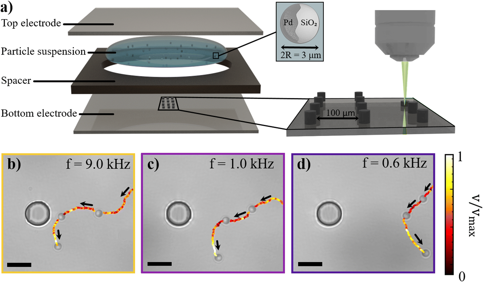

Fig. 1 Synthetic microswimmers turn away from obstacles. (a) Our experimental system: we study the active motion of 3 μm SiO₂ Janus colloids with thin Pd caps self-propelling under an AC electric field. We place the colloids in water between two transparent conductive surfaces separated by a spacer and connected to a function generator, and image particle motion with an inverted microscope. The bottom surface, parallel to which colloids self-propel, is patterned with 3D-printed obstacles in various configurations. Upon approach, the active particles reorient and avoid the obstacle surface due to tunable long-range repulsive interactions. Microscopy images obtained at a fixed 6 V peak-to-peak amplitude and frequency (b) 9.0 kHz, (c) 1.0 kHz, and (d) 0.6 kHz, illustrating the turning-away response. Trajectories are colored according to the normalized instantaneous velocity of the particle. Scale bars are 10 μm.

At field frequencies f between 100 Hz and 10 kHz, similar to the ones tested here, metallo-dielectric Janus colloids self-propel due to asymmetric electrodynamic flows generated along their surfaces.^56,57 In this frequency range, the period of the applied electric field, T = 1/f, lies between two key charge relaxation times: the charge relaxation time of the electric double layer (EDL) at the electrode interface, τ_e = λ₀H/D (where D is the electrolyte diffusivity and λ₀ is the Debye screening length), and the charge relaxation time of the particle, τ_p = λ₀R/D. This implies that the EDL at the electrode interface builds up only partially, while there is sufficient time for the metallic cap of the Janus particle to fully polarize in response to the electric field. The resulting polarization induces a charge distribution on the particle surface. The interaction between the applied electric field and this induced charge gives rise to electrohydrodynamic (EHD) flows around the particle through induced-charge electro-osmosis (ICEO).^58–60 If the particles were compositionally symmetric, the flows around them would be symmetric and quadrupolar,⁶¹ resulting in no motion. However, due to different polarizability of the metallic and dielectric sides of the particles, there exists an asymmetric induced charge distribution and thus an imbalance in the electrohydrodynamic flows between the two sides, causing self-propulsion with the metallic half at the back. Under the conditions applied in our experiments this leads to self-propulsion velocities ranging between 12 and 20 μm s⁻¹, see Fig. S1 in the ESI.†

We first examine the effect of a single cylindrical obstacle on approaching microswimmers, and find that they change their motion direction and turn away from the obstacle. Example active trajectories that illustrate this effect are shown in Fig. 1(b)–(d) and Video S1 (ESI†).

Specifically, at a frequency of f = 9.0 kHz, the particle “senses” the obstacle and avoids it, see Fig. 1(b). We find that this behavior persists for a range of frequencies, see f = 1.0 kHz in Fig. 1(c) and f = 0.6 kHz in Fig. 1(d), albeit with “sensing” and turning away taking place at increasingly larger distances. We observe that, at low frequencies, particles slow down as they swim towards the obstacle and subsequently reorient and swim away with a higher speed (see the trajectories color-coded according to the instantaneous self-propulsion velocity in Fig. 1 and quantification of the average self-propulsion velocity versus radial distance from the pillar in Fig. S2 in the ESI†). Sufficiently far away from the obstacle, particles recover their frequency-dependent swimming speed. We note that at frequencies f ≫ 9.0 kHz the particle self-propulsion effectively ceases until at f ≤ 50 kHz the Janus particles start moving with their metallic caps oriented forward.⁶⁰ In this frequency range, the metallic caps of the Janus particles exhibit a strong attraction toward the pillar when in close proximity, leading to its immobilization at the pillar surface.

We now focus on the sub-kHz to low-kHz frequency range to investigate in detail how the applied frequency influences particle dynamics. To this end, we quantify microswimmer –boundary interactions at applied frequencies ranging from f = 0.4 kHz to f = 9.0 kHz, where repulsive behavior is observed (see Fig. 2(a)–(c)). We compute time-averaged particle density profiles around the obstacles (see Methods and Fig. 2(d)–(f) for representative examples). In these maps, dark regions correspond to a high probability of finding a particle, whereas light regions indicate low probability.

Fig. 2 Tunable long-ranged microswimmer–obstacle interaction through adjusting the applied field frequency, f. Bright-field microscopy images with active colloids in proximity to a cylindrical obstacle (diameter 10 μm, height 6 μm) under a fixed 6 V peak-to-peak amplitude and f of (a) 9.0 kHz, (b) 1.0 kHz, and (c) 0.6 kHz. (d)–(f) Time-averaged particle density profiles around the obstacle corresponding to a–c, normalized by the time-averaged density in the sample far away from the obstacle. (g) Particle-obstacle separation distance r₉₀, defined as the distance at which the normalized time-averaged microswimmer density is equal to 0.9, as a function of f. Inset shows the normalized particle density as a function of radial distance from the obstacle for f = 0.6 kHz, 1.0 kHz, and 9.0 kHz. The dotted line indicates the extracted r₉₀ value. Scale bars are 10 μm.

At a frequency of f = 9.0 kHz, we do not observe any apparent exclusion region around obstacles, as in Fig. 2(d). However, as we decrease the frequency of the electric field to 1.0 kHz in Fig. 2(e) and 0.6 kHz in Fig. 2(f), a well-defined exclusion region appears, indicating an increase in the effective size of the obstacle. Using the corresponding time-averaged density profiles, we calculate the normalized average particle density at each distance from the obstacle surface and at different frequencies. We show example curves that correspond to frequencies of f = 9.0, 1.0 and 0.6 kHz in the inset of Fig. 2(g). We subsequently extract the distance from the obstacle where the time-averaged density profile equals 0.9, corresponding to a 90% probability for a microswimmer to be able to reach the corresponding distance from the obstacle (represented by a horizontal dotted line, r₉₀, in the inset of Fig. 2(g)). Plotting the extracted r₉₀ values as a function of f in the main panel in turn reveals a monotonically-decreasing separation distance with increasing frequency. Detailed data at various frequencies within the f = 0.6–9.0 kHz range can be found in Fig. S3 in the ESI.†

The data in Fig. 2(g) are well fitted with the expression , with a = 6.7 ± 0.2 and c = 2.2 ± 0.2, μm for this specific sample (see dashed line). Notably, the inverse relationship between field frequency and the size of the exclusion region around the obstacles is remarkably robust, persisting across Janus particles with varying core materials, metal caps and sizes, as shown in Fig. S4 in the ESI.† A similar dependence of the exclusion region on f is also observed for bare 3 μm SiO₂ spheres, i.e., non-self-propelling ones. However, these spheres exhibit a larger exclusion zone compared to their metallic-capped counterparts (see Fig. S6 in the ESI†). It is worth noting that the self-organization of bare, passive spheres differs from that of the active Janus spheres, particularly in the low-frequency regime where bare particles form large aggregates,^57,59 potentially affecting the observed exclusion zones.

The qualitative robustness of the frequency-dependent exclusion zone surrounding the cylindrical obstacle and its scaling point at the presence of EHD flows induced by the dielectric pillar residing on the bottom electrode. In the absence of the obstacle, the applied electric field causes counterions to migrate toward the electrodes and co-ions to be repelled, resulting in the formation of an electric double layer near the electrodes. Consequently, the charges on each electrode are balanced by those in the diffuse layer, and the fluid remains stationary. However, when the dielectric obstacle is introduced, it induces an electric field gradient, with a component tangential to the bottom electrode. This disturbance causes the charges within the electrode polarization layer to move, driving fluid motion, commonly referred to as EHD flow.

The observed inverse relationship between the applied field frequency and the size of the exclusion zone surrounding the pillars aligns with theoretical predictions by Ristenpart et al.,⁶² who demonstrated that the strength of EHD flows induced by a dielectric object near a conductive surface decreases with increasing field frequency. We use tracer particle analysis (see Fig. S5 and Video S4 in the ESI†) to visualize the flow field around the pillars in our system and confirm outward-directed hydrodynamic flows along the substrate whose maximum velocity, v_max, scales as . These observations further support that EHD flows cause the repulsive interactions between the pillars and Janus particles, as we schematically depict in the insets in Fig. S5b–d in the ESI.† Additionally, the presence of electric field gradients will also generate dielectrophoretic (DEP) forces. To evaluate their importance, we have calculated their magnitude as a function of radial distance from the pillar (see Section S7 and Fig. S7 in the ESI†). The DEP force exerted on the dielectric core of the Janus particles by the pillar is repulsive, remains approximately constant across different frequencies, and is shorter ranged than the EHD flow field. Therefore, we do not expect DEP to contribute to particle repulsion strongly. In contrast, the DEP force acting on the metallic cap of the Janus particles is attractive across the entire range of investigated frequencies (see Fig. S8 in the ESI†). While we do not expect this contribution to significantly affect the magnitude of the DEP force on the Janus colloid – DEP forces scale with volume and the volume of the dielectric core is much larger than the volume of the metallic cap – this attractive interaction may contribute to the characteristic turning-away behavior observed as Janus particles approach the pillar, potentially in combination with hydrodynamic coupling between the outward monopolar flow field generated by the pillar (Fig. S5b–d, ESI†) and the quadrupolar flow field around the metallo-dielectric Janus microswimmers.^60,61

In practical terms, the discussion above implies that a simple adjustment of the frequency allows for fine-tuning the size of the exclusion zone around the cylindrical obstacles in our experiments, transforming each obstacle into a ‘soft’ repulsive boundary whose effective size can be dynamically controlled.

We observe that the size of the exclusion zone also depends on the strength of the applied field (see Fig. S9 in the ESI†). Specifically, at lower frequencies, (r₉₀) decreases as the field strength increases. This contrasts with the expected quadratic increase in the magnitude of EHD flows as a function of applied voltage, suggesting that at higher frequencies, the self-propulsion force of the Janus particles – which increases significantly – begins to play a more dominant role in determining how closely can the microswimmers approach the pillar. In this manuscript, however, we focus on tuning the interactions by varying the frequency of the applied field, which enables broad control over the effective size of the obstacles while maintaining a relatively constant self-propulsion speed.

2.2. Microswimmer gating in patterned environments

The frequency-dependent effective obstacle size allows us to tune the behavior and self-organization of our active particles across different environments patterned with obstacles. We fabricate lattice configurations with different patterns, and vary both the spacing between neighboring obstacles as well as the effective obstacle size dynamically through frequency modulation, as established above.

First, we examine active motion within straight arrays of obstacles with lattice spacing of 10 μm in the x direction and 35 μm in the y direction. We find that at a frequency f = 9.0 kHz, particles move through the obstacle arrays without any preferred direction. In Fig. 3(a), we overlay example particle trajectories on top of a micrograph depicting the obstacle array and show that the active colloids are able to explore the environment unimpeded, as also evidenced by the distribution of directions in the particle displacements in the inset. As shown in Fig. 2(d), the effective obstacle size at this frequency is very similar to its physical dimensions and substantially smaller than the gaps between the obstacles, so the particles can easily swim between them. However, note that this case is different from the one of catalytically-active particles which are captured by obstacles.^{33–38,48–51}

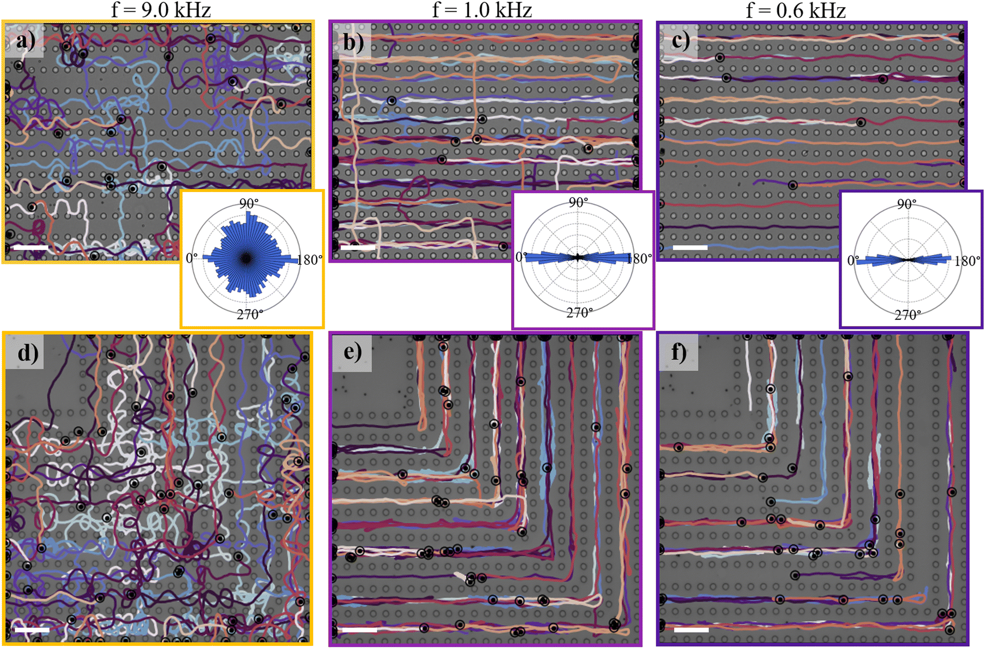Fig. 3 Tunable microswimmer gating across environments with obstacles in straight and bent path configurations. Representative active trajectories of colloids self-propelling through arrays of cylindrical obstacles with a lattice spacing of 10 μm in the x and 35 μm in the y direction, at varying applied frequency f of (a) 9.0 kHz, (b) 1.0 kHz, and (c) 0.6 kHz. Insets show the distributions of directions in the displacements of the particles over 1 s intervals, extracted from at least 60 trajectories of 2 min duration. Representative active trajectories of colloids self-propelling through an obstacle array with a lattice spacing of 10 μm in the x and 35 μm in the y direction constructed to form a path with a 90° bend, at f of (d) 9.0 kHz, (e) 1.0 kHz, and (f) 0.6 kHz. The peak-to-peak field amplitude is fixed in all experiments at 6 V. Scale bars are 50 μm.

At a frequency f = 1 kHz, particles instead move predominantly in straight paths in the x direction parallel to the obstacle array, and rarely cross along in the y direction (Fig. 3(b)). This behavior becomes even more pronounced at frequency f = 0.6 kHz (Fig. 3(c)), where active particles only appear to move along the x direction and in the middle of the obstacles, which now effectively act as channels. This is further reflected in the distribution of directions, see the corresponding insets, as follows from Fig. 2(e)–(g). In those two cases, the separation between the obstacle columns is smaller than the effective obstacle size reported in Fig. 2(d), such that the gaps between obstacles in the y direction are effectively closed, while providing a guiding action in lanes in the x direction. Tuning the effective obstacle size thus allows us to gate active particle motion along specific directions.

This frequency-dependent gating also enables guiding particles along more complex paths, i.e. around sharp bends. In Fig. 3(d)–(f) and Video S2 (ESI†), we add a 90° bend in the same lattice as previously described and, as before, we observe that at frequency f = 9 kHz, our active colloids freely explore the obstacle lattice and actively distribute themselves across the entire available space (Fig. 3(d)). Adjusting the frequency to f = 1.0 kHz (Fig. 3(e)) and to f = 0.6 kHz (Fig. 3(f)), again prevents particles from crossing across different rows in the lattice and forces them to follow obstacle lines, also around the bends, indicating that our frequency-dependent gating allows directing particles within complex environments, suggestive of analogies to liquid gating technologies.⁶³

2.3. Tunable microswimmer confinement in disordered environments

Finally, the gating strategy reported above gives us the opportunity to tune and directly control the confinement of active particles inside environments with a broad distribution of separations between obstacles, which we print here to form a 2D disordered environment. We show representative active trajectories obtained from 2 min recordings within these disordered environments in Fig. 4(a)–(c) and Video S3 (ESI†). Already from the trajectories, we see that tuning the applied field frequency leads to particle localization.

Fig. 4 Tunable confinement of synthetic microswimmers within disordered environments. Representative trajectories of active colloids within a disordered array of 3D-printed obstacles under a fixed peak-to-peak voltage of V_pp = 6 V, and frequency f of (a) 9.0 kHz, (b) 1.0 kHz, and (c) 0.6 kHz. Trajectories are overlaid on top of a bright-field image of the patterned environment. Circles with black dots represent the active colloids in the last frame of the 2 min recording of their trajectories. Insets show corresponding mean squared displacements of individual colloids (IMSDs, 〈Δr²〉) as a function of lag time τ. (d)–(f) Time-averaged microswimmer density profiles corresponding to (a)–(c). Each dataset represents an average over 16 measurements with a duration of 4 min. Obstacles are plotted as light grey circles with dark grey edge lines. Changing the frequency increases the effective size of the obstacles, as discussed earlier, creating closed paths, where the distance between obstacle surfaces d is smaller than the corresponding r₉₀ value (marked by a red line connecting the obstacles). Insets show the distribution of nearest distance between obstacle surfaces, subtracted by the r₉₀ value of the corresponding frequency. Values of d − r₉₀ below 0 (black dashed line) correspond to closed paths, plotted as red bars in the distribution, whereas open paths are plotted as blue bars. Scale bars are 100 μm.

At a frequency f = 9.0 kHz, the trajectories of the swimmers approach the obstacles closely such that they can cross all gaps between the obstacles freely and explore all available space (Fig. 4(a)). However, upon changing frequency to f = 1.0 kHz in Fig. 4(b), a given fraction of gaps, i.e those for which the distance between obstacles becomes smaller than r₉₀, is effectively closed for the particles, which limits the regions they can explore. This effect becomes more pronounced when we lower the frequency further to f = 0.6 kHz in Fig. 4(c). The occurrence of gating strongly influences active trajectories, as clearly shown by the mean square displacements of individual colloids as a function of lag time reported in the insets. In the presence of restrictions in space exploration, plateaus in the mean square displacements emerge as microswimmers become caged inside the larger cavities and cannot escape through the gaps between the obstacles.

This frequency-dependent caging is clearly visualized by evaluating time-averaged microswimmer density maps under various applied frequencies, see Methods and Fig. 4(d)–(f). In particular, we mark closed gaps, which microswimmers cannot cross, with a red line that connects neighboring obstacles in Fig. 4(e) and (f) corresponding to f = 1.0 and f = 0.6 kHz, respectively. The number of closed paths in the system increases with decreasing frequency, as shown in the distribution reported in the inset. Specifically, the blue bars in the distribution correspond to open, permitted paths and red bars to closed ones following to the corresponding values of r₉₀.

3. Conclusions

In summary, we demonstrate that we can engineer long-range interactions between colloids self-propelling under an electric field and obstacles configured in prescribed paths forming complex tunable environments. As a result of these interactions, active colloids turn away from obstacles and avoid accumulation at boundaries, showing a distinctive difference from the classically-observed behavior for catalytic synthetic microswimmers. By dynamically varying the effective obstacle size we can achieve gating and confinement of active colloids via a modulation of the gaps between obstacles that can be easily opened and closed.

The precise and rapid regulation strategy that we describe here offers high potential for the dynamic control of active particle gating, and bypasses key limitations of previous studies that utilized catalytically self-propelled colloids in topographically-patterned environments. In particular, by introducing feedback schemes that connect gating to real-time particle distributions, we envisage future work towards motion rectification, dynamic sorting of particles based on motility, and creation of tunable self-assembled active particle patterns. We therefore propose that electric fields open up exciting avenues for manipulating synthetic active matter in complex environments giving access to interaction modes with confinement geometries that expand existing possibilities towards the realization of advanced autonomous active units.

4. Materials and methods

4.1. Janus particles

Metallo-dielectric Janus colloids are fabricated by drop-casting an aqueous suspension of SiO₂ spheres (2R = 2.96 μm, SiO2-R-LSC84, microparticles GmbH) on a plasma-cleaned microscopy slide, followed by depositing a thin (2 nm) Cr adhesion layer and a 6.5 nm Pd layer. The resulting Janus spheres were dispersed in 50 mL Milli-Q water, and washed 3 times by centrifugation and redispersion in fresh Milli-Q water. Finally, the particles were concentrated to a volume of 0.5 mL to obtain a suspension of approximately 2 mg particles per mL solution. For the Janus particles with varying sizes, core materials, and metallic caps, the same fabrication procedure was applied using the following core-cap combinations: SiO₂ spheres with diameter 2R = 2.06 μm (SiO2-R-L1561, microparticles GmbH) coated with a 6.5 nm Pd hemispherical layer, SiO₂ spheres with diameter 2R = 2.96 μm (SiO2-R-LSC84, microparticles GmbH) coated with an 8.0 nm Au hemispherical layer, and polystyrene spheres with diameter 2R = 2.99 μm (PS-FluoRed-Fi306, microparticles GmbH) coated with a 6.5 nm Pd hemispherical layer.

4.2. Patterned environments

Microstructures were produced with a nanoscribe photonic professional GT2, which uses two-photon lithography. Designs comprised cylindrical obstacles with height 6 μm and diameter 10 μm in various configurations, and were designed using a CAD software (Autodesk Fusion) and processed with describe. Obstacles were printed onto UV-ozone treated ITO-coated glass slides (Nanoscribe) using the commercial photoresist IP-S as a pre-polymer. Standard printing parameters were selected, as specified by the manufacturer: the printer was equipped with a 25×-immersion objective (Zeiss, NA = 0.8) and used to print in DiLL mode. After printing, the structures were developed by submersion in propylene glycol methylether acrylate for 15 min, immediately followed by gently dipping into isopropyl alcohol and gentle drying with a nitrogen gun. This procedure reliable removes the unpolymerized photoresist. All micro-patterning steps were performed under yellow light. Finally, the printed structures were post-cured for 6 min under a UV lamp with wavelength 565 nm.

4.3. Preparation of the experimental cell

Prior to the experiments a small amount of the Janus particle suspension was mixed in a 1 : 1 ratio with a 2% surfactant (pluronic-127, Sigma Aldrich) solution. A 5 μL droplet of the suspension was placed in a custom-made sample cell consisting of two transparent electrodes separated by an adhesive spacer with a 9 mm-circular opening and 120 μm height (Grace Bio-Labs SecureSeal). The bottom electrodes were decorated with obstacles as described above and the top ones were plain ITO-coated slides cleaned via 20 min sonication in acetone and Milli-Q water, followed by drying with a pure nitrogen stream before assembling the sample cell. Once the particles were added and the electrodes adhered via the spacer, the electrodes were connected using copper tape to a function generator (National Instruments Agilent 3352X) that applies the AC electric field (f = 0.6–9.0 kHz, V_pp = 6 V).

4.4. Imaging

The sample cell was mounted on an Eclipse Ti2 inverted microscope in bright-field mode and videos were recorded at a frame rate of 10 frames per second using a CMOS camera (Orca Flash 4.0 V3, Hammamatsu). Data for particle density mapping were obtained using a 4× objective (Plan Fluor 4×, Nikon, NA = 0.13) with 1.5 magnification lens. In addition, higher magnification data were obtained for particle tracking and Janus cap visualization using 20× (S plan fluor 20×, Nikon, NA = 0.45) and 40× (S Plan Fluor 40×, Nikon, NA = 0.60) objectives.

4.5. Particle tracking

The acquired images were preprocessed in Python by inverting their intensity values and binarizing them to enhance the contrast between obstacles and the background. The centers of the obstacles were identified in the binarized images using OpenCV. Obstacle detection was achieved by applying an area threshold to select features within the desired size range. Once identified, obstacle regions were masked out from the images to exclude them from further analysis. Particle tracking was then performed on the remaining masked images using a centroid finding algorithm implemented in Python (Trackpy).^64,65

4.6. Time-averaged density maps around single obstacles

For the time-averaged density maps around obstacles, we followed the same preprocessing procedure as described above. However, instead of tracking the particles, the masked images were overlaid. To obtain the density profiles shown in Fig. 2 as well as Fig. S3 and S6 (ESI†), 16 image sequences with a field of view of 102 × 102 pixels, each lasting 2 minutes and recorded at 10 fps, were overlaid. The images were normalized by the mean pixel value calculated from the 10 pixels along the edges of the time-averaged image. For the density profiles shown in Fig. 4, data from 16 experiments, each lasting 4 minutes with a field of view of 550 × 550 pixels, were overlaid based on the best alignment of the obstacle centers in the corresponding image sequences. The resulting density maps were normalized by the time-average pixel intensity measured 50–55 μm away from the disordered lattice.

4.7. Tracer particle experiments

For the tracer particle experiments, the experimental cell was prepared as described above; however, instead of the Janus particle suspension, a suspension containing fluorescent polystyrene spheres (2R = 200 nm, 0.5 mg mL⁻¹) was added to the sample cell. Data were acquired as described above using a 60× objective (S Plan Fluor 60×, Nikon, NA = 0.70) in fluorescence mode. Optical flow analysis was then performed on the acquired frames using the Farnebäck algorithm⁶⁶ implemented in OpenCV Version 4.4.0.⁶⁷ Consecutive frame pairs were processed to compute the dense optical flow fields using the following algorithm parameters: pyramid scale = 0.5, number of pyramid levels = 3, window size = 15, iterations = 3, polynomial expansion size = 8, and standard deviation = 1.2. The resulting velocity vectors were averaged over time to obtain a mean flow field, and the flow magnitude was extracted from the horizontal and vertical components.

Author contributions

Conceptualization: C. v. B., L. I. and S. K. Formal analysis: A. T., C. v. B. and I. G. Funding acquisition: L. I. Investigation: A. T., C. v. B., I. G. and S. K. Methodology: C. v. B., I. G., L. I. and S. K. Project administration: L. I. Software: C. v. B. and I. G. Supervision: S. K. and L. I. Validation: C. v. B., S. K. and I. G. Visualization: C. v. B., S. K. and L. I. Writing – original draft: C. v. B. and S. K. Writing – review and editing: C. v. B., I. G., L. I. and S. K.

Data availability

The data supporting this article have either already been included as part of the ESI,† or will be included upon publication.

Conflicts of interest

The authors declare that they have no conflicts of interests.

Acknowledgements

The authors thank Moran Bercovici for discussions on electrokinetic phenomena and Robert Style for support on data analysis. C. v. B. acknowledges funding from the European Unions Horizon 2020 MSCA-ITN-ETN, project number 812780. L. I., S. K. and C. v. B. acknowledge funding from the European Research Council (ERC) under the European Unions Horizon 2020 Research and innovation program grant agreement no. 101001514.

References

1. S. Moreno-Gámez, R. A. Sorg, A. Domenech, M. Kjos, F. J. Weissing, G. S. van Doorn and J.-W. Veening, Nat. Commun., 2017, 8, 854.
2. P. P. Lele, B. G. Hosu and H. C. Berg, Proc. Natl. Acad. Sci. U. S. A., 2013, 110, 11839–11844.
3. A. Persat, C. D. Nadell, M. K. Kim, F. Ingremeau, A. Siryaporn, K. Drescher, N. S. Wingreen, B. L. Bassler, Z. Gitai and H. A. Stone, Cell, 2015, 161, 988–997.
4. B.-J. Laventie and U. Jenal, Annu. Rev. Microbiol., 2020, 74, 735–760.
5. J. Singh, A. Pagulayan, B. A. Camley and A. S. Nain, Proc. Natl. Acad. Sci. U. S. A., 2021, 118, e2011815118.
6. B. Lin, T. Yin, Y. I. Wu, T. Inoue and A. Levchenko, Nat. Commun., 2015, 6, 6619.
7. L. Hall-Stoodley, J. W. Costerton and P. Stoodley, Nat. Rev. Microbiol., 2004, 2, 95–108.
8. C. K. Lee, J. Vachier, J. de Anda, K. Zhao, A. E. Baker, R. R. Bennett, C. R. Armbruster, K. A. Lewis, R. L. Tarnopol, C. J. Lomba, D. A. Hogan, M. R. Parsek, G. A. O'Toole, R. Golestanian and G. C. L. Wong, mBio, 2020, 11, 1.
9. W. R. DiLuzio, L. Turner, M. Mayer, P. Garstecki, D. B. Weibel, H. C. Berg and G. M. Whitesides, Nature, 2005, 435, 1271–1274.
10. K. Drescher, J. Dunkel, L. H. Cisneros, S. Ganguly and R. E. Goldstein, Proc. Natl. Acad. Sci. U. S. A., 2011, 108, 10940–10945.
11. V. Kantsler, J. Dunkel, M. Polin and R. E. Goldstein, Proc. Natl. Acad. Sci. U. S. A., 2013, 110, 1187–1192.
12. C. Berne, C. K. Ellison and A. Ducret, Nat. Rev. Microbiol., 2016, 18, 616–627.
13. E. Lauga and T. R. Powers, Rep. Prog. Phys., 2009, 72, 096601.
14. J. Elgeti, R. G. Winkler and G. Gompper, Rep. Prog. Phys., 2015, 78, 056601.
15. R. Dreyfus, J. Baudry, M. L. Roper, M. Fermigier, H. A. Stone and J. Bibette, Nature, 2005, 437, 862–865.
16. R. Golestanian, T. B. Liverpool and A. Ajdari, Phys. Rev. Lett., 2005, 94, 220801.
17. C. Bechinger, R. D. Leonardo, H. Löwen, C. Reichhardt, G. Volpe and G. Volpe, Rev. Mod. Phys., 2016, 88, 045006.
18. A. Zöttl and H. Stark, J. Phys.: Condens. Matter, 2016, 28, 253001.
19. J. Katuri, X. Ma, M. M. Stanton and S. Sánchez, Acc. Chem. Res., 2017, 50, 2–11.
20. D. Patra, S. Sengupta, W. Duan, H. Zhang, R. Pavlick and A. Sen, Nanoscale, 2013, 5, 1273–1283.
21. K. Han, C. W. S. Iv and O. D. Velev, Adv. Funct. Mater., 2018, 28, 1705953.
22. M. García, J. Orozco, M. Guix, W. Gao, S. Sattayasamitsathit, A. Escarpa, A. Merkocic and J. Wang, Curr. Opin. Colloid Interface Sci., 2013, 5, 1325–1331.
23. L. Restrepo-Pérez, L. Soler, C. Martínez-Cisneros, S. Sánchez and O. G. Schmidt, Lab Chip, 2014, 14, 2914.
24. W. Gao, R. Dong, S. Thamphiwatana, J. Li, W. Gao, L. Zhang and J. Wang, ACS Nano, 2015, 9, 117–123.
25. J. Wang, Z. Xiong, J. Zheng, X. Zhan and J. Tang, Acc. Chem. Res., 2018, 51, 1957–1965.
26. H. Ceylan, I. C. Yasa, O. Yasa, A. F. Tabak, J. Giltinan and M. Sitti, ACS Nano, 2019, 13, 3353–3362.
27. W. Gao, X. Feng, A. Pei, Y. Gu, J. Li and J. Wang, Nanoscale, 2013, 5, 4696–4700.
28. Q. Wang, F. Ji, D. S. Wang and L. Zhang, ChemNanoMat, 2021, 7, 600.
29. D. Xu, H. Yuan and X. Ma, ChemNanoMat, 2021, 7, 439–442.
30. S. J. Ebbens, Curr. Opin. Colloid Interface Sci., 2016, 21, 14–23.
31. K. J. Bishop, S. L. Biswal and B. Bharti, Annu. Rev. Chem. Biomol. Eng., 2023, 14, 1–30.
32. A. C. H. Tsang, E. Demir, Y. Ding and O. S. Pak, Adv. Intell. Syst., 2020, 2, 1900137.
33. M. Mijalkov and G. Volpe, Soft Matter, 2013, 9, 6376–6381.
34. J. Katuri, D. Caballero, R. Voituriez, J. Samitier and S. Sánchez, ACS Nano, 2018, 12, 7282–7291.
35. C. Maggi, J. Simmchen, F. Saglimbeni, J. Katuri, M. Dipalo, F. D. Angelis, S. Sanchez and R. D. Leonardo, Small, 2015, 12, 446–451.
36. C. O. Reichhardt and C. Reichhardt, Annu. Rev. Condens. Matter Phys., 2017, 8, 51–75.
37. A. Kaiser, H. H. Wensink and H. Löwen, Phys. Rev. Lett., 2012, 108, 268307.
38. L. S. Palacios, S. Tchoumakov, M. Guix, I. Pagonabarraga, S. Sánchez and A. G. Grushin, Nat. Commun., 2021, 12, 4691.
39. S. J. Ebbens and J. R. Howse, Langmuir, 2011, 27, 12293–12296.
40. A. I. Campbell and S. J. Ebbens, Langmuir, 2013, 29, 14066–14073.
41. S. Ketzetzi, J. de Graaf and D. J. Kraft, Phys. Rev. Lett., 2020, 125, 238001.
42. M. R. Bailey, C. M. B. Gutiérrez, J. Martín-Roca, V. Niggel, V. Carrasco-Fadanelli, I. Buttinoni, I. Pagonabarraga, L. Isa and C. Valeriani, Nanoscale, 2024, 16, 2444–2451.
43. V. Carrasco-Fadanelli and I. Buttinoni, Phys. Rev. Res., 2023, 5, L012018.
44. S. Das, A. Garg, A. I. Campbell, J. Howse, A. Sen, D. Velegol, R. Golestanian and S. J. Ebbens, Nat. Commun., 2015, 6, 8999.
45. J. Simmchen, J. Katuri, W. E. Uspal, M. N. Popescu, M. Tasinkevych and S. Sánchez, Nat. Commun., 2016, 7, 10598.
46. H. Yu, A. Kopach, V. R. Misko, A. A. Vasylenko, D. Makarov, F. Marchesoni, F. Nori, L. Baraban and G. Cuniberti, Small, 2016, 12, 5882–5890.
47. C. Liu, C. Zhou, W. Wang and H. P. Zhang, Phys. Rev. Lett., 2016, 117, 198001.
48. D. Takagi, J. Palacci, A. B. Braunschweig, M. J. Shelley and J. Zhang, Soft Matter, 2014, 10, 1784.
49. A. T. Brown, I. D. Vladescu, A. Dawson, T. Vissers, J. Schwarz-Linek, J. S. Lintuvuori and W. C. K. Poon, Soft Matter, 2016, 12, 131–140.
50. C. van Baalen, W. E. Uspal, M. N. Popescu and L. Isa, Soft Matter, 2023, 19, 8790–8801.
51. S. Ketzetzi, M. Rinaldin, P. Dröge, J. de Graaf and D. J. Kraft, Nat. Commun., 2022, 13, 1772.
52. M. S. D. Wykes, X. Zhong, J. Tong, T. Adachi, Y. Liu, L. Ristroph, M. D. Ward, M. J. Shelley and J. Zhang, Soft Matter, 2017, 13, 4681–4688.
53. V. M. S. G. Tanuku, P. Vogel, T. Palberg and I. Buttinoni, Soft Matter, 2023, 19, 5452–5458.
54. M. Trivedi, D. Saxena, W. K. Ng, R. Sapienza and G. Volpe, Nat. Phys., 2022, 18, 939–944.
55. C. W. Shields and O. D. Velev, Chem, 2017, 3, 539–559.
56. T. M. Squires and M. Z. Bazant, J. Fluid Mech., 2006, 560, 65–101.
57. W. Ristenpart, I. A. Aksay and D. Saville, J. Fluid Mech., 2007, 575, 83–109.
58. F. Ma, X. Yang, H. Zhao2 and N. Wu, Phys. Rev. Lett., 2015, 115, 208302.
59. X. Yang, S. Johnson and N. Wu, Adv. Intell. Syst., 2019, 1, 1900096.
60. A. Boymelgreen, G. Kunti, P. Garcia-Sanchez, A. Ramos, G. Yossifon and T. Miloh, J. Colloid Interface Sci., 2022, 616, 465–475.
61. T. M. Squires and M. Z. Bazant, J. Fluid Mech., 2004, 509, 217–252.
62. W. Ristenpart, I. A. Aksay and D. Saville, Phys. Rev. E: Stat., Nonlinear, Soft Matter Phys., 2004, 69, 021405.
63. S. Yu, L. Pan, Y. Zhang, X. Chen and X. Hou, Pure Appl. Chem., 2021, 93, 1353–1370.
64. J. C. Crocker and D. G. Grier, J. Colloid Interface Sci., 1996, 179, 298–310.
65. D. B. Allan, T. Caswell, N. C. Keim and C. M. van der Wel, trackpy: Trackpy v0.4.1, 2018 DOI:10.5281/zenodo.1226458.
66. G. Farnebäck, Proceedings of the 13th Scandinavian Conference on Image Analysis, 2003, pp. 363-370.
67. G. Bradski, Dr Dobb's Journal of Software Tools, 2000.

---

Footnotes

† Electronic supplementary information (ESI) available: Experimental videos and corresponding description. See DOI: https://doi.org/10.1039/d4sm01512f

‡ These authors contributed equally to this work.

§ Present address: John A. Paulson School of Engineering and Applied Sciences, Harvard University, Cambridge, MA 02138, USA.

---