
 Open Access Article
 This Open Access Article is licensed under a
 Creative Commons Attribution 3.0 Unported Licence
In silico environmental chemical science: properties and processes from statistical and computational modelling
Paul G.
Tratnyek
 *a,
Eric J.
Bylaska
b and
Eric J.
Weber
c
*a,
Eric J.
Bylaska
b and
Eric J.
Weber
c
aInstitute of Environmental Health, Oregon Health & Science University, 3181 SW Sam Jackson Park Road, Portland, OR 97239, USA. E-mail: tratnyek@ohsu.edu
bWilliam R. Wiley Environmental Molecular Sciences Laboratory, Pacific Northwest National Laboratory, P.O. Box 999, Richland, WA 99352, USA
cNational Exposure Assessment Laboratory, U.S. Environmental Protection Agency, 960 College Station Road, Athens, GA 30605, USA
First published on 24th February 2017
Abstract
Quantitative structure–activity relationships (QSARs) have long been used in the environmental sciences. More recently, molecular modeling and chemoinformatic methods have become widespread. These methods have the potential to expand and accelerate advances in environmental chemistry because they complement observational and experimental data with “in silico” results and analysis. The opportunities and challenges that arise at the intersection between statistical and theoretical in silico methods are most apparent in the context of properties that determine the environmental fate and effects of chemical contaminants (degradation rate constants, partition coefficients, toxicities, etc.). The main example of this is the calibration of QSARs using descriptor variable data calculated from molecular modeling, which can make QSARs more useful for predicting property data that are unavailable, but also can make them more powerful tools for diagnosis of fate determining pathways and mechanisms. Emerging opportunities for “in silico environmental chemical science” are to move beyond the calculation of specific chemical properties using statistical models and toward more fully in silico models, prediction of transformation pathways and products, incorporation of environmental factors into model predictions, integration of databases and predictive models into more comprehensive and efficient tools for exposure assessment, and extending the applicability of all the above from chemicals to biologicals and materials.
Environmental impactComputational models are used in all aspects of environmental science, including assessment of the environmental fate and effects of chemical substances. In these applications, the prediction of missing property data is the main motivation, but prediction of pathways (e.g., products from contaminant degradation) is becoming feasible and should soon be available for use in research and regulation. The degree to which substance impact assessment can be done in silico will continue to increase, but incorporation of environmental factors (i.e., conditions) is a continuing challenge. |
Introduction
Progress in environmental chemical science is limited by the availability of data even more than most domains of science. The complexity of environmental conditions, combined with the diversity of substances (chemical, biological, and material) that are of environmental concern, mean that direct measurements will never be sufficient to meet the data needs of environmental scientists or regulators. Therefore, predicting chemical properties is a long-standing challenge that has received extensive study for many applications (chemical engineering, green chemistry, environmental chemistry, toxicology, pharmacology, etc.). Fortunately, advances in computer-based methods are making it increasingly feasible to estimate substance properties, evaluate their fate-determining processes, and predict their effects. These methods and their applications comprise the domain we refer to herein as “in silico environmental chemical science”. The scope of this domain includes theoretical and statistical methods for calculating substance properties, fate, and effects. The theoretical and statistical methods used to calculate substance properties are rooted in very different disciplines, so the recent trend toward combining these approaches poses some novel challenges for developers and users of these models. One goal of this perspective is to show how these challenges become opportunities when methods are combined in a complementary way. To encourage this, we provide an overview of some core concepts, key developments, and opportunities, with emphasis on the properties that are the most fundamental determinants of chemical fate and effects. Another perspective in this issue1 takes a similar approach, but focuses on biological effects, especially toxicity, and their regulatory implications.We framed the introduction to this perspective in terms of prediction of substance properties because that is by far the most familiar rationale for work in this area. For example, comprehensive exposure assessment models for chemical contaminants that are used for regulatory decision making (EXAMS,2 EUSES,3 FOCUS,4etc.) require dozens of chemical properties, for which measured values often are not available, hence the widely-recognized need for methods of estimating the missing data.5,6 The demand for methods that estimate environmental substance properties has mostly been met with statistical models, including “quantitative structure–activity relationships” (QSARs) and variations thereof.7–10 This field is mature enough to have already engendered several generations of compilations of predictive models.6 Prominent early examples are the Handbook of Chemical Property Estimation Methods compiled by Lyman et al.,11 and a similarly structured volume edited by Mackay and Boethling.12 Since then, there has been a growing number of reviews and databases of QSARs,13–17 comparative analyses of QSAR accuracy,18–20 and efforts to codify methods of calibration and validation.21–25 Many QSARs have been incorporated into software that facilitates their use for property prediction.6 Currently, the two main examples of this are the estimation program interface (EPI Suite) by the U.S. Environmental Protection Agency (EPA)26,27 and the QSAR Toolbox by the Organization for Economic Cooperation and Development (OECD),28 but others are under development.
However, the approach taken in this perspective is broader in that it recognizes that property prediction models, and the processes and methods of developing these models, have additional benefits. Besides prediction, another major benefit is “diagnostic”, as in the diagnosis of mechanisms, categories, or other structures that provide greater understanding of the processes at issue. In chemistry, this process is generically referred to as correlation analysis,29,30 and it often takes the specific form of linear free energy relationships (LFERs).31,32 A third benefit, which sometimes is neglected, is for the validation of data (or models). The process of developing QSARs involves analysis of correlations, which should be simple if the variables are closely related, so scatter and outliers may be indicative of errors or bias.
Formulation of statistical models
In the past, and even now, almost all property prediction models have been based on empirical/statistical correlations between data for the response (target, dependent, y) variable and descriptor (independent, x) variable(s), as illustrated in Fig. 1. For training the model, the response variable is usually measured data (e.g., toxicity) and the descriptor variable may be measured or determined in other ways (e.g., various fragment types such as Hammett substituent constants). The statistical model usually is relatively simple (linear, with one or a few descriptor variables) and is derived through calibration: i.e., regression of available property data for a series of related compounds with one, or several, convenient descriptor variables. Usually, a subset of the training data set, or entirely new data, are used to validate the model. The resulting relationship can be used in reverse to predict values of the property for compounds that were not included in the original data set. The general paradigm represented in Fig. 1 still applies for more complex systems and models. | ||
| Fig. 1 Conceptual model for the process of calibration, validation, and prediction using statistical models such as quantitative structure–activity relationships (QSARs). Only one response and one descriptor variable is represented by this 2-D scatter plot, but multivariable models work similarly. | ||
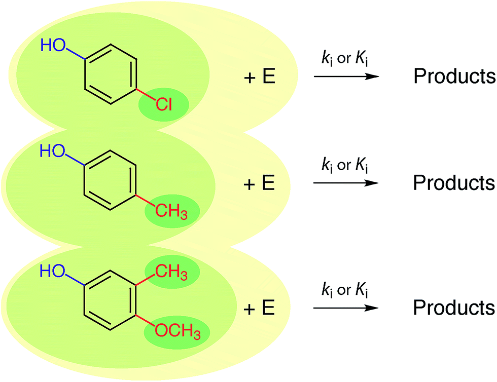
In practice, the response variable is defined by external considerations (e.g., constants required for modelling partitioning or degradation of contaminants) and the development of the predictive model involves mostly the identification of descriptor variables and calibration of the relationship between them. With respect to the selection of descriptor variables for chemical processes, there are three general types: (i) substituent constants such as the σ constants that are defined and used with correlations in the form of the Hammett equation, (ii) molecular descriptors such as pKa the way they are used in the Brönsted equation, and (iii) reaction descriptors such as in the correlation of rate or equilibrium constants in one medium with those in another (i.e., “cross-correlations”, see below). These three categories of descriptors are illustrated in Fig. 2, using as an example rate constants (ki) for a reaction of substituted phenols with an environmental agent E. The environmental agent E could be O3, MnO2, a (co)metabolizing microorganism, etc. The distinction made in Fig. 2 between substituent, molecular, and reaction descriptors could be generalized for application to other types of environmental processes (e.g., volatilization, sorption, bioavailability, and toxicity).
 | ||
| Fig. 2 Summary of the relationship between three major types of descriptor variables for chemical reactions. The three shades of coloured ovals represent substituents (dark), molecules (medium), and reactions (light). E represents the controlling environmental factor in the reaction (e.g. irradiance in photolysis, pH in hydrolysis, ozone concentration in disinfection, etc.), and is similar to the y-axis in Fig. 6. | ||
The three types of descriptors represented in Fig. 2 have complementary advantages and disadvantages. The main advantage of the substituent approach is that constants for a limited number of substituents can be combined to provide values of the descriptor variable for new, more complex substrate molecules. However, not all substances can be adequately represented as the sum of independent substituents, due to proximity effects, etc. Correlations based on molecular properties are not limited by uncertainties over the additivity of substituent effects because values of their descriptor variables are determined on whole molecules, thereby incorporating the effects of interacting substituents. Correlations based on substituent or molecular properties do not include information about the reaction pathway or products, whereas this information may be incorporated in descriptor variables based on reaction properties. Again, there are advantages and disadvantages to the alternatives: if pathways or products are unresolved in the response variable data (e.g., using overall k's or K's measured in environmental media), there may not be sufficient information to select descriptor variables that correspond to specific reactions, but selection of substituent or molecular property descriptors does not require that information. On the other hand, if there is a need to resolve different pathways and products (e.g., to distinguish environmentally benign and harmful outcomes), then correlations based on descriptors that include information about reactions and products (i.e., the whole reaction) are required.
A variation on the model represented by Fig. 2 is the format sometimes called “cross-correlation analysis” where two variables that typically would be response variables are related directly (e.g., rate constants for reaction with one oxidant vs. rate constants for reaction with another).13,14,33 Cross-correlations can be used for prediction, validation, and classification, just like conventional QSARs.
Matching response and descriptor variables
The potential scope of in silico environmental chemical science includes phenomena ranging in scale from angstroms to kilometers. This continuum is illustrated in Fig. 3 with representative categories for both physical–chemical (left column) and biological–chemical (right column) systems. At the molecular end of this continuum, the system characteristics are relatively simple, in that they are fundamental and homogeneous (e.g., rate constants for electron transfer between donor and acceptor molecules in solution). At the environmental end of this continuum, system characteristics are relatively complex and heterogeneous (e.g., toxicity to a diverse community of organisms). All of these systems' characteristics are legitimate targets (as response variables) for predictive and/or diagnostic in silico modelling, depending on the context or purpose, such as whether the application is ranking of contaminants for regulation or tuning a treatment technology to produce less harmful by-products.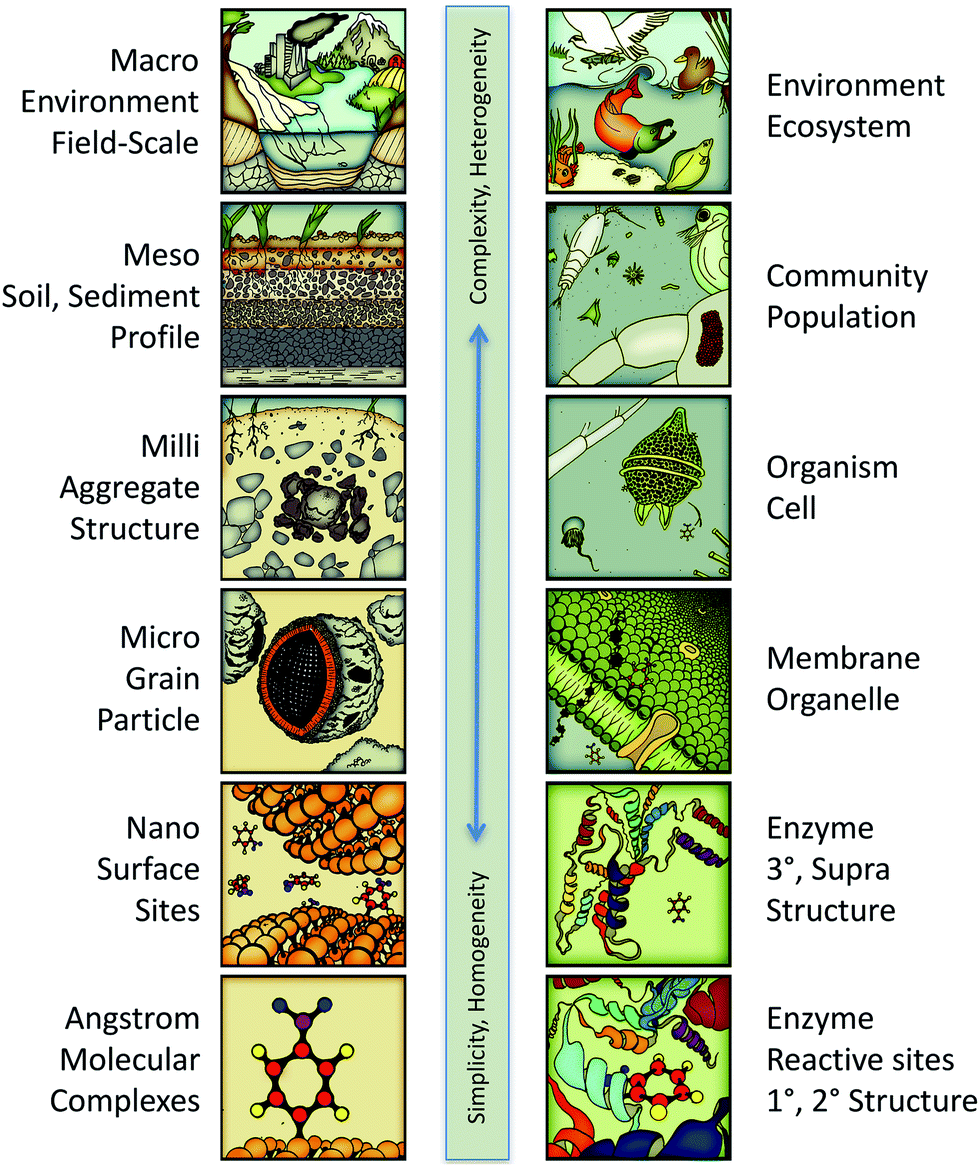 | ||
| Fig. 3 Continuum of system scales encompassing the whole potential scope of predictive/diagnostic modelling for in silico environmental chemical sciences. Left column: The physical–chemical categories are similar to those in multi-scaling models of geochemical processes.34 Right column: The biological–chemical categories are adapted from a multi-scaling diagram by Damborsky.35 | ||
Just as different response variables correspond to different positions on the scale continuum in Fig. 3, a similar classification applies to descriptor variables. So, for example, the redox potential of reactants corresponds to molecular scale processes, its octanol–water partition coefficient corresponds to membrane/grain scale processes, and its toxicity corresponds to the cell or community scales. As with the selection of response variables, valid descriptor variables may come from anyplace on the scaling continuum. However, the most easily justified and interpreted models are formulated with response and descriptor variables from similar scales. Thus, redox potential is a well-matched descriptor for response variables involving redox reaction rates and partition coefficients are well matched for modelling bioavailability.
This principle of matching the physical scale of response and descriptor variables also applies to scale in the more abstract sense, as in the distinction made in Fig. 2 between substituent, molecular, and reaction level descriptors. As noted in the discussion of that figure, the three types of descriptors can be more or less effective depending on the type (scale) of descriptor that they are matched with. A specific and even more fundamental example of matching as a criterion on selecting response and descriptor variables can be found in the discussion of descriptors for oxidation of phenols and anilines by Pavitt et al.36 There the distinction was between descriptors that are properties measured in solution vs. descriptors that are calculated from theory assuming an elementary reaction step. The latter is more precisely defined, but may not fully match the solution chemistry that determines the response variable. In contrast, measured descriptor variables usually are less precisely defined, but this imprecision can make them more effective in QSARs, if the source of the imprecision is in some way shared by (covariant between) the descriptor and response variables.
Toward the larger-scale end of the continuum represented in Fig. 3, response variables for more complex or heterogeneous processes often are best described with multivariate “polyparameter” models comprised of combinations of descriptors for smaller scale steps that comprise the overall process. In these cases, the key consideration for descriptor selection is not so much matching but rather balancing the smaller scale processes represented by each descriptor. The classic example of this is the Hansch–Fujita model, which represents biological effects with a linear combination of descriptors for partition and reaction processes.37–39 A more recent example is the Abraham model, which represents partitioning effects in terms of descriptors for all of the factors that influence the partitioning process.40–43 For balance, these descriptors should represent distinct, largely-independent (i.e., not overlapping or covariant) factors. In a case like the Abraham equation, the descriptors are also balanced by representing similar scale effects; for models representing more complex effects, like the Hansch–Fujita equation, a balanced set of descriptors may represent effects over a range of scales.
For complex, large-scale processes and effects, statistical predictive/diagnostic models must be based on correlations between empirical data. However, for molecular scale processes and effects, an alternative to empirical data for descriptor variables is calculation from molecular structure theory (i.e., computational chemistry). While this approach has great appeal because of the potential to alleviate the need for field or laboratory measurement, and for the high “precision” of theoretically calculated descriptors discussed above, the computational chemistry approach comes with other complications and limitations that limit its potential as an alternative to statistical correlation analysis.
Modelling from computational chemistry
Computational chemistry involves molecular modelling based on theory.44 Starting from quantum mechanics, all chemical phenomena can—in principal—be calculated from theory,45 but solving the exact equations directly is infeasible except for very small systems. To overcome this obstacle, many methods have been developed for approximating the difficult equations of quantum mechanics, so that they can be solved for molecular systems. The most promising of these methods rely on sophisticated combinations of two general strategies: (i) use of compact models that capture the key many-particle effects by construction and (ii) efficient stochastic sampling of many-dimensions. There are many variations on these methods, which collectively make up the toolbox of computational chemistry (Fig. 4). Some of these methods are easily performed on modern computers, and therefore are available to most environmental chemists, but other methods require advanced computers and applied mathematical techniques, and therefore remain the domain of computation chemistry specialists.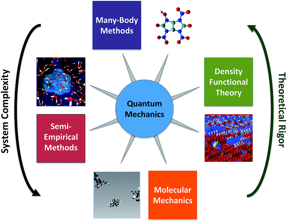 | ||
| Fig. 4 Summary of computational chemistry methods, with respect to their theoretical rigor, and therefore potential accuracy, versus the complexity of systems they can address, and therefore relevance to environmental chemistry issues at different scales. | ||
The simplest computational chemistry models are based on molecular mechanics, in which the forces between the atoms are calculated using empirical interatomic potentials or molecular mechanical force fields.46,47 The computational efficiency of these models makes it practical for them to simulate the dynamics and coupled interactions of tens of thousands of molecules over time-scales of milliseconds,48 which makes it possible to study molecular behaviour in complex environmental phases. For example, molecular mechanics models have been used to investigate the structure of natural organics matter,49–51 and interactions of contaminants with mineral–water interfaces.52–54 A major limitation to the use of molecular mechanics modelling, however, is that the required force field parameters are not very accurate for effects that are relevant to environmental conditions, such as the strong polarization and other chemical interactions of surrounding water molecules near highly charged ions and complex mineral surfaces.55,56 Moreover, current molecular mechanics models typically are not designed to simulate chemical reactions (i.e., the making and breaking of chemical bonds) or phenomena that are kinetically limited over time frames that exceed a few microseconds.46 Solutions to these limitations are active areas of research in computational chemistry and applied mathematics (e.g. ReaxFF57 and “accelerated sampling” techniques46,47,58) and recent advances in computational algorithms allow the integration over time to be parallelized, thereby allowing for increased simulation time-scales.59,60
Semi-empirical methods are more complex than molecular mechanics models, and include simplified approximations of quantum mechanics that are sufficient to allow simulation of the making and breaking of bonds during chemical reactions. These methods often use an simplified Hamiltonian to model organic systems,61,62 although more general Hamiltonians have been developed to model other parts of the periodic table.62,63 Unlike the more rigorous computational models discussed below, semi-empirical methods are heavily parameterized with experimental data (or data from higher level models). This allows semi-empirical models to efficiently achieve useful accuracy for large molecules (>10![[thin space (1/6-em)]](https://www.rsc.org/images/entities/char_2009.gif) 000 atoms with O(N) algorithms64), although for small molecules or reaction energies the more rigorous models usually are more accurate. There are many examples of using semi-empirical methods in the early applications of computational chemistry to environmental systems, mostly for descriptor variables in calibration of QSARs.65–71
000 atoms with O(N) algorithms64), although for small molecules or reaction energies the more rigorous models usually are more accurate. There are many examples of using semi-empirical methods in the early applications of computational chemistry to environmental systems, mostly for descriptor variables in calibration of QSARs.65–71
Currently, the most popular approximation to quantum mechanics for chemistry is Density Functional Theory (DFT),72–74 which is based on approximations to the exact exchange–correlation functional73 (e.g. LDA, GGA, hybrid GGA, meta-GGA) that are relatively computationally efficient. DFT's success and popularity can be attributed to several advantages it has over other contemporary computational chemistry approaches: the Hohenberg–Kohn theorem75 and Kohn–Sham formulations74 give it a well-established theoretical basis, many of the most popular exchange correlation functionals are constrained by formal theoretical constraints, it is competitive in accuracy for many interesting chemical phenomena, and it is computationally much less expensive than higher-level alternatives such as quantum Monte-Carlo methods and traditional many-body theory (discussed below). DFT has been used extensively in many research domains, including environmental chemistry.
While the DFT level of approximation is suitable for many applications, it is also becoming clear after many years of active development that there are limits to its accuracy. For example, the DFT calculated free energies of reaction for reactions involving bond breaking can have uncertainties of several kcal mol−1 or more.76,77 If the reaction occurs in aqueous solution, popular models of solvent effects (i.e. implicit solvent models) will contribute at least a few more kcal mol−1 of uncertainty,44 so overall errors of 5 kcal mol−1 (∼20 kJ mol−1) or more are to be expected. This level of accuracy is not satisfactory for some purposes (e.g., direct calculation of absolute values of specific rate constants for contaminant degradation78), but it may be satisfactory for triaging among possible chemical reaction pathways or for descriptor data in QSAR development.79,80 In addition, the overall accuracy of DFT calculations can be improved by using methods that make use of empirical additivity rules for molecular properties, where various properties of larger molecules can be thought of as being made up of additive contributions of atoms, bonds, or collections of atoms and bonds (i.e., functional groups) of the molecule.81,82 These approaches have proven to be effective for small organic molecules,83–90 and recently they have been used in advanced computational algorithms that can be used to simulate extremely large molecules, even including complex proteins and DNA chains.91,92
Compared with DFT, the higher level theory used in wave function and quantum Monte-Carlo methods93 can give significantly more accurate results, if the underlying electronic structure is well understood. For small molecules, higher level wave function methods, such as coupled cluster theory and its variants94,95 are currently considered the most accurate many-body methods in use today. However, the computational cost of these methods increases very steeply with molecular size, such that only molecules containing a few atoms can be handled currently. Despite their high computational cost, many-body methods have the potential to considerably increase the accuracy of the study of many molecular phenomena (except for a few well-known exceptions96,97) and there has recently been significant progress made at accelerating and parallelizing these methods.98 For systems composed of numerous small molecules that are difficult to study by experiment—as is often the case in environmental chemistry—modelling with many-body methods is feasible and attractive (because a large number of benchmark studies have shown that the errors of many-body methods are considerably smaller than for DFT, ranging from <1 kJ mol−1 to up to 3 kJ mol−1, depending on the species86,99−101).
An approach that combines some of the advantages of the methods summarized above—and is especially useful for describing chemical reactivity in large-scale, complex environments—is the quantum mechanical/molecular mechanical (QM/MM) methodology. In this approach, the system is divided into two parts: a localized QM region surrounded by a MM region. In many applications, this allows for a small chemically active region to be modelled quantum mechanically, while the long-range effects (such as solvent or a protein backbone) can be represented by classical MM interactions. This is a computationally efficient and theoretically powerful method, but uncertainties in how best to divide the QM and MM regions of the model make it the domain of “expert” users, for now. Applications of QM/MM methods to environmental chemistry are still relatively few.102–105
Empirical calibration of computational chemistry data with experimental data
While few properties that directly impact the environmental fate and effects of substances can be calculated directly from molecular structure theory, properties that can be calculated from theory can be useful in the development of statistical models. Usually, these calculated properties are used as descriptor variable data in correlations with measured response variable data, so the resulting relationship has many of the same characteristics as traditional LFERs and QSARs (Fig. 1). These calculated descriptor variables can be substituent, molecular, or reaction properties (as in Fig. 2), they generally are computationally feasible only for molecular size-scale properties, and their selection is subject to the same considerations of matching and balance discussed above for traditional QSARs (Fig. 3). The major advantages of computationally derived descriptor variables are that they can be programmed to calculate in large batches and they include only the effects they are programmed to model. The latter is also their major disadvantage: they do not include any effects that are not already known to be relevant, or effects that are not practical to calculate from theory.This mixture of advantages and disadvantages can be seen in the growing body of research done on QSARs using descriptors from computational chemistry. One such class of descriptors includes physico-chemical properties (solubility, Henry's law constants, partitioning constants) calculated using the conductor-like screening models COSMO-RS,106–108 COSMOtherm,109,110 and COSMO-SAC.111–113 These are poly-parameter statistical models40 using combinations of parameters that are balanced (i.e., mechanistically complementary and independent) and calculated based (partly) on theory.
Another class of descriptors that are obtained from computational chemistry calculations includes one-electron oxidation or reduction potentials (E1), which are used in QSARs for rates of contaminant degradation by redox reactions.79,80,114,115 In this case, the calculated potentials require calibration using experimental data, and the experimental calibration data can be measured by several methods, including electrochemistry and pulse radiolysis. The electrochemical measurements can be confounded by non-ideal behaviour, such as irreversibility, which are not included in the theoretical calculations, so there is a mismatch between these two variables that might result in less accurate calibrations.116,117 Alternatively, E1 measured by pulse radiolysis,114,115,117–119 is a better estimate of reversible redox potentials, and therefore is better matched to potentials calculated from computational chemistry. However, E1 from pulse radiolysis is not necessarily more closely matched to the processes that are controlling solution-phase oxidation kinetics, so they may not provide the most useful, or even the most accurate, structure–activity relationships for oxidation reactions of environmental interest.36
In principle, this approach could be extended to “fully in silico” calibration of QSARs: i.e., statistical correlations calibrated with descriptor and response variable data calculated from molecular modelling. This was the original goal in a study of the hydrolysis and reduction of nitro aromatic compounds78,80 and oxidation of their corresponding aromatic amines.79 However, complexity and uncertainty in the mechanism of the hydrolysis and oxidation reactions made it infeasible to calculate their rates entirely from theory, and even the comparatively well-defined and simple mechanism of reduction proved challenging to model for more than a few compounds.80
Pathway as opposed to property prediction
A relatively new challenge that has emerged in recent years is the ability to predict transformation pathways as a function of environmental conditions. This is partly due to growing recognition that the resulting transformation products can be of more concern than the parent compound with respect to ecological and human toxicity. Our understanding of the process science underlying abiotic and biologically-mediated transformations has progressed to the point that it is now feasible to construct reaction libraries that “encode” the process science that is described in the peer-reviewed literature or publicly available government regulatory documents. The resulting libraries represent reactions as single-step transformations of functional groups, and can include purely chemical reactions (e.g., hydrolysis, reduction, and photolysis) and biologically-mediated processes (i.e., aerobic and anaerobic biodegradation and human metabolism).The development of reaction libraries is accomplished by the use of reaction transform languages such as SMIRKS and SMARTS,120 in conjunction with cheminformatics software tools. The execution of these reaction libraries predicts the major transformation pathways and their products. Although well-developed tools that execute reaction libraries for human metabolism are commercially available, currently only one tool is available for executing reaction libraries that predict environmental fate (enviPath121–123), and this tool currently contains rules only for aerobic biodegradation. Additional software and libraries for predicting contaminant pathways and products are under development, such as for ozonation of micropollutants under water treatment conditions.124,125
A common challenge to developers of tools to predict transformation pathways is to minimize the prediction of irrelevant transformation products, sometimes referred to as the “combinatorial explosion”, which has been defined as the prediction of many irrelevant transformation products when transformation pathways are iteratively applied to predict consecutive transformation reactions.126 Strategies that have been used to minimize the problem of combinatorial explosion include assignment of likelihoods to the generalized transformation pathways in a defined reaction library,126 a relative reasoning approach,126 a combined absolute and relative approach,127 a hybrid knowledge and machine learning-based approach,121 and an approach based on the development of reaction rules for selectivity, reactivity, and exclusion.
Fig. 5 provides an example of a reaction scheme for the hydrolysis of halogenated aliphatics (RX) containing vicinal halogens through HX elimination, and shows how this reaction scheme can be pruned by use of rules for selectivity as well as reactivity. In this example, the reaction scheme predicts that hydrolysis of 1,2-dibromo-3-chloropropane (DBCP) could yield four products; however, only one hydrolysis product (2-bromo-3-chloropropene) is predicted when rules for selectivity are included, which is consistent with experimental results.128 The reactivity rule states the order of removal of halogens (labeled reactant atom 3 in the reaction scheme) is inverse to their atomic number (i.e., I > Br > Cl > F), because the carbon–halogen bond strength is greatest for the most electrophilic halogen.129 Execution of this selectivity rule—which states the hydrogen attached to the β-carbon having the fewest hydrogen substituents is preferentially eliminated130—predicts that elimination of the hydrogen in the 2-position of DBCP is the only major pathway.
 | ||
| Fig. 5 Example of pathway prediction with rules for reactivity and selectivity, showing initial steps for dehalogenation of 1,2-dibromo-3-chloropropane (DBCP) by elimination. Four products are predicted by the generalized reaction scheme, but pruning with reactivity and selectivity rules predicts only one major product, 2-bromo-3-chloropropene. | ||
An additional challenge to the developers of these tools is the need to incorporate the effect of environmental conditions on rates and pathways for many classes of chemicals. For example, it has been well documented how changes in pH can have significant effects on both the rates and hydrolysis pathways of organophosphorus triesters in aquatic ecosystems.129 This need to account for environmental conditions is discussed in greater detail below.
Incorporating environmental conditions
In so far as the ultimate goal of in silico environmental chemical science is describing the fate/effects of substances in real/outdoor environments, it is not always sufficient to model only response variables that are formulated as fundamental properties with the effects of environmental conditions largely factored out. However, leaving too many environmental effects factored into the response variable will limit the applicability of the model to environments with different conditions. Conceptually, the ultimate solution to this dilemma is to incorporate both substance and environmental properties into the model as descriptor variables of the overall response variable. These three types of variables correspond to the x, y, and z in the conceptual model shown in Fig. 6.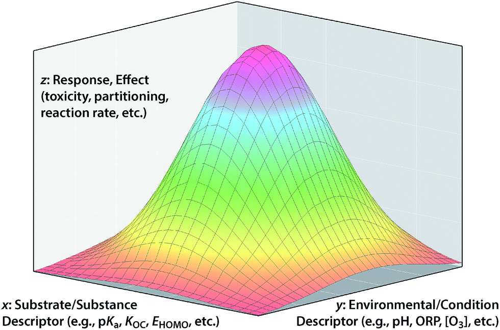 | ||
| Fig. 6 Conceptual model for 3-dimensional QSARs with response variable on the z-axis, substance property on the x-axis and environmental properties on the y-axis. Traditional QSARs correspond to a cross-section of the surface in the x–z plan. The drawing is not based on any particular data so the surface shape is arbitrary and the axes are not numbered. | ||
An example that clearly fits the conceptual model shown in Fig. 6 is the overall bioavailability (response variable, z) of a class of contaminants of soil and sediment that comes in complex mixtures (e.g., PCBs, PCDDs, PAHs). In this example, one independent variable axis (x) represents the range of properties of the family of congeners (e.g., Koc of different PCBs) and the other independent variable (y) represent the range of environmental conditions (e.g., quantity and composition of sorptive phases in the sediment across a site). An application of the conceptual model in Fig. 6 to degradation of contaminants is exemplified by work on the natural attenuation of chlorinated hydrocarbon (CHC) solvents in groundwater.131,132 In that case, the overall response is the decrease in total contaminant load (in terms of concentration, equivalent toxicity, etc.); the environmental descriptor is the type and quantity of reducing materials that can dechlorinate the contaminants (iron oxides, sulfides, microorganisms, etc.) and the contaminant descriptor is the reactivity of each contaminant with the various reductants (i.e., specific rate constants). The area under the surface could be the overall decrease in contaminant concentration at a site, or rate of decrease in concentration, change in equivalent toxicity, etc. depending on exactly how the response variable is formulated.
A traditional 2-D QSAR corresponds to a cross section through Fig. 6 in the x–z plane, for a particular y. In principle, a QSAR through the y–z plane can be defined at a particular x (e.g., dechlorination of one CHC by environmental phases with different reduction potentials), but this is a challenging frontier with few examples at this time. Ultimately, it would be desirable to fully define whole response surfaces such as those shown in Fig. 6, but this also is impractical with current methods. Progress toward the ultimate goal of QSARs that represent both substance and environmental properties has been limited, and the relatively few attempts to do that illustrate the challenges that arise. For example, rates of contaminant reduction in anoxic sediments have been described with a polyparameter QSAR that includes descriptors of both contaminant properties and sediment conditions,133 but there is too much uncertainty over how to parameterize the environmental factors in such models for them to predict absolute rates of contaminant reduction in sediments with confidence.
While the full conceptual model represented by Fig. 6 is difficult to parameterize with specific data, general consideration of the model can provide some useful insights into the process of QSAR formulation. An example of this involves the fungibility of factor allocation among the three types of variables, which is a key aspect of the “art” of formulating successful QSARs, and a manifestation of the principles of matching and balancing described above. By fungibility, we mean that one arrangement of factor allocations sometimes can be replaced by another with similar results. For a specific example of this, consider the strategy of developing QSARs using response variables that are normalized to data for a reference substance in order to remove variability in the data due to experimental or environmental conditions.14,79,134 This strategy effectively collapses the surface in Fig. 6 into a conventional 2-D QSAR by moving the information about environmental conditions from the y into the z axis. However, implicit in this strategy is the assumption that environmental effects are uniform across the range of QSARs based on substance descriptor variables (i.e., that the relationship in Fig. 6 is a flat plane not curved surface), and this is not always true.79
Integration of databases, pathway prediction systems, and chemical property predictors
The primary role of chemical exposure assessment models used for regulatory decision making is to provide estimated environmental concentrations (EECs) of the chemical of interest and its potential transformation products in environmental media. Examples of models that calculate EECs for pesticide exposures include FIRST (FQPA Index Reservoir Screening Tool), GENEEC2 (GENeric Estimated Environmental Concentration), and SWCC (Surface Water Concentration Calculator). The parameterization of these models requires chemical properties and knowledge of the dominant transformation products formed from the environmental transformation of the parent chemical as a function of environmental conditions. The data submitted for the chemical registration process prescribed by environmental laws—such as the Toxic Substances Control Act (TSCA); Federal Insecticide, Fungicide, and Rodenticide Act (FIFRA); and the Registration, Evaluation, Authorization and Restriction of Chemicals (REACH) regulations—are typically measured in media specific systems. For example, the rates and transformation product formation for chemically-mediated transformation processes such hydrolysis and photolysis are measured in water under pH controlled conditions and biologically-mediated processes such as aerobic and anaerobic biodegradation are measured in soils and sediments. In reality, transformation pathways such as hydrolysis and abiotic reduction in anoxic sediments, photolysis and hydrolysis in aquatic ecosystems, and aerobic biodegradation and hydrolysis in aerobic soils, will occur simultaneously.The parameterization of exposure assessment models requires the development of integrated tools that reflect this reality (i.e., have the ability to provide the data required for the estimation of environmental concentrations as a function of environmental conditions).135,136 The hallmarks of an integrated tool for predicting environmental transport and transformation include (i) seamless connection to databases of measured and calculated chemical properties and chemical pathway prediction systems; (ii) calculation of chemical properties based on the execution of multiple property calculators and prediction of transformation pathways based on environmental conditions; (iii) simultaneous execution of multiple reaction libraries based on specific transformation pathways; (iv) parameterization and execution of QSARs for the calculation of transformation rate constants; (v) high through-put analyses (i.e., run in batch mode), and (vi) open access to the general public.
Movement towards web-based databases and tools, and development of the software technologies that will enable seamless calls to these systems through web-based services, is accelerating the development of integrated computational systems. This ability for seamless linkage will reduce the need for duplicative efforts, resulting in significant savings of resources and time. Examples of databases and pathway prediction systems that are currently web-based, or are currently being updated as web-based tools include EPA's ICSS Chemistry Dashboard,137,138 CEFIC's AMBIT,139 OECD's Toolbox,28 and EAWAG's enviPath.121,122 The ICSS Chemistry Dashboard is a web-based data base for ∼700000 chemicals that maps curated physicochemical property data associated with chemical substances to their corresponding chemical structures. EnviPath is an aerobic biodegradation reaction library based on 332 biotransformation descriptions for 249 biotransformation rules. Web services are currently being developed for enviPath.
To address the need for a fully integrated tool, EPA's Office of Research and Development is currently developing the Chemical Transformation Simulator (CTS), with release to the general public planned for late 2017. The primary components of the CTS are a Physico-Chemical Property Calculator (PPC) and a Reaction Pathway Simulator (RPS) (Fig. 7). The PPC will allow the user to compare properties generated by a variety of calculators that take different approaches to estimating specific physicochemical properties. The calculators currently implemented include EPI Suite, which uses a fragment-based approach; TEST (Toxicity Estimation Software Tool), which uses QSAR-based approaches; and ChemAxon plug-in calculators, which use an atom-based fragment approach. The output derived from these calculators will enable the user to compare the calculated data with measured data extracted from readily accessible web-based databases (e.g., ICSS Chemistry Dashboard).
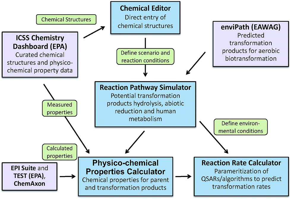 | ||
| Fig. 7 Major components of the Chemical Transformation Simulator including Chemical Editor, the Reaction Pathway Simulator. Links to enviPath provide the ability to generate transformation products resulting from aerobic biotransformation. Links to the ICSS Chemistry Dashboard provide additional calculated and measured chemical properties, as well as curated chemical structures. | ||
The RPS allows the user to select individual or multiple reaction libraries dependent on the environmental media of interest. The beta version of the CTS has reaction libraries for hydrolysis, reduction, and human metabolism. A reaction library for photolysis is currently under development and will be available for the fully functional version of the CTS. This updated version of the CTS will have the ability to execute a reaction library of aerobic biodegradation through seamless linkage to the EAWAG PPS using web services that are currently being developed for this tool.
A Reaction Rate Calculator (RRC) is also under development for the fully functional version of the CTS. The RRC will provide for the parametrization and subsequent execution of QSARs for the prediction of transformation rates. Currently, rate constants for transformation processes represent a significant data gap for the parameterization of models used for estimating environmental concentration. The RRC will be limited by the availability of existing QSARs and the ability to construct new QSARs for this purpose.
Future prospects
The scope of this perspective reflects the maturity of traditional statistical QSAR methods for predicting the environmental fate/effects determining properties of chemicals; the great potential of theoretical/computational chemistry methods for improving the prediction of chemical properties or characterization of transformation pathways; and the transformative impact of integrating QSAR and molecular models, with informatic and internet tools, to make predictive modelling more accessible, efficient, and comprehensive. The emphasis on chemical contaminants reflects the balance of focus of most work on development and application of in silico models in environmental chemical science to date. However, some of the methods and results developed for modelling chemical fate and effects in the environment should also apply to other substances. This is evident in the still young but rapidly developing application of QSARs to materials, especially nanoparticles.140–145 An even greater challenge lies in the extension of QSAR methods to biological properties like virulence (i.e., virulence factor activity relationships, VFARs).146–148 The challenges involved in implementing useful VFARs are considerable, but may eventually succumb to the combination of advances from computational toxicology1 and omic sciences.149Disclaimer
The views expressed in this article are those of the author(s) and do not necessarily represent the views or policies of the U.S. Environmental Protection Agency or other sponsoring agencies. Mention of trade names or products does not convey, and should not be interpreted as official EPA approval, endorsement, or recommendation.Acknowledgements
The authors acknowledge input on this manuscript from Kathrin Fenner and J. Samuel Arey. The artwork in Fig. 3 is by Brittany Cummings. The authors' work in this area is supported by the U.S. National Science Foundation (NSF grants 1333476 and 1506744), Department of Defense (SERDP grants ER-1735 and 2725), Department of Energy (EMSL project DE-AC06-76RLO 1830), and Environmental Protection Agency.References
- M. T. D. Cronin, (Q)SARs to predict environmental toxicities: current status and future needs, Environ. Sci.: Processes Impacts, 2017 10.1039/c6em00687f.
- L. A. Burns, D. M. Cline and R. R. Lassiter, Exposure analysis modeling system (EXAMS): User manual and system documentation, U.S. Environmental Protection Agency, Athens, GA, 1982, EPA-600/3-82-023 Search PubMed.
- European Union System for the Evaluation of Substances, http://ec.europa.eu/jrc/en/scientific-tool/european-union-system-evaluation-substances, accessed 1/1/2017.
- EU FOCUS Work Group on Degradation Kinetics, Generic Guidance for Estimating Persistence and Degradation Kinetics from Environmental Fate Studies on Pesticides in EU Registration (Ver. 1.1), 2014, Sanco/10058/2005 Search PubMed.
- W. T. Donaldson, The role of property–reactivity relationships in meeting the EPA's needs for environmental rate constants, Environ. Toxicol. Chem., 1992, 11, 887–891, DOI:10.1002/etc.5620110702.
- M. L. Card, V. Gomez-Alvarez, W.-H. Lee, D. G. Lynch, N. S. Orentas, M. Titcombe Lee, E. M. Wong and R. S. Boethling, History of EPI Suite™ and future perspectives on chemical property estimation in US Toxic Substances Control Act new chemical risk assessments, Environ. Sci.: Processes Impacts, 2017 10.1039/c7em00064b.
- Recent Advances in QSAR Studies: Methods and Applications, ed. T. Puzyn, J. Leszczynski and M. T. D. Cronin, Springer, Dordrecht, 2010, DOI:10.1007/978-1-4020-9783-6.
- M. Nendza, Structure–Activity Relationships in Environmental Sciences, Chapman & Hall, Dordrecht, 1998, DOI:10.1007/978-1-4615-5805-7.
- Quantitative Structure–Activity Relationships in Environmental Sciences—VIII, ed. F. Chen and G. Schüürmann, Society of Environmental Toxicology and Chemistry, Pensacola, FL, 1997 Search PubMed.
- C. Hansch and A. Leo, Exploring QSAR, Fundamentals and Applications in Chemistry and Biology, American Chemical Society, Washington, DC, 1995 Search PubMed.
- W. J. Lyman, W. F. Reehl, D. H. Rosenblatt, W. F. Reehl and D. H. Rosenblatt, Handbook of Chemical Property Estimation Methods, McGraw-HillLyman, W.J., New York, 1982 Search PubMed.
- Handbook of Property Estimation Methods for Chemicals: Environmental and Health Sciences, ed. D. Mackay and R. S. Boethling, Lewis, Boca Raton, FL, 2000 Search PubMed.
- S. Canonica and P. G. Tratnyek, Quantitative structure–activity relationships for oxidation reactions of organic chemicals in water, Environ. Toxicol. Chem., 2003, 22, 1743–1754, DOI:10.1897/01-237.
- P. G. Tratnyek, E. J. Weber and R. P. Schwarzenbach, Quantitative structure–activity relationships for chemical reductions of organic contaminants, Environ. Toxicol. Chem., 2003, 22, 1733–1742, DOI:10.1897/01-236.
- L. Mamy, D. Patureau, E. Barriuso, C. Bedos, F. Bessac, X. Louchart, F. Martin-Laurent, C. Miege and P. Benoit, Prediction of the fate of organic compounds in the environment from their molecular properties: a review, Crit. Rev. Environ. Sci. Technol., 2015, 45, 1277–1377, DOI:10.1080/10643389.2014.955627.
- T. M. Nolte and A. M. J. Ragas, Review of quantitative structure–property relationships for fate of ionizable organic chemicals in water matrices and identification of knowledge gaps, Environ. Sci.: Processes Impacts, 2017 10.1039/c7em00034k.
- C. Nieto-Draghi, G. Fayet, B. Creton, X. Rozanska, P. Rotureau, J.-C. de Hemptinne, P. Ungerer, B. Rousseau and C. Adamo, A general guidebook for the theoretical prediction of physicochemical properties of chemicals for regulatory purposes, Chem. Rev., 2015, 115, 13093–13164, DOI:10.1021/acs.chemrev.5b00215.
- Z. Fu, J. Chen, X. Li, Y. n. Wang and H. Yu, Comparison of prediction methods for octanol–air partition coefficients of diverse organic compounds, Chemosphere, 2016, 148, 118–125, DOI:10.1016/j.chemosphere.2016.01.013.
- J. Devillers, P. Pandard and B. Richard, External validation of structure–biodegradation relationship (SBR) models for predicting the biodegradability of xenobiotics, SAR QSAR Environ. Res., 2013, 24, 979–993, DOI:10.1080/1062936x.2013.848632.
- E. R. Bennett, J. Clausen, E. Linkov and I. Linkov, Predicting physical properties of emerging compounds with limited physical and chemical data: QSAR model uncertainty and applicability to military munitions, Chemosphere, 2009, 77, 1412–1418, DOI:10.1016/j.chemosphere.2009.09.003.
- A. Racz, D. Bajusz and K. Heberger, Consistency of QSAR models: correct split of training and test sets, ranking of models and performance parameters, SAR QSAR Environ. Res., 2015, 26, 683–700, DOI:10.1080/1062936x.2015.1084647.
- J. Devillers, Methods for building QSARs, Methods Mol. Biol., 2013, 930, 3–27, DOI:10.1007/978-1-62703-059-5_1.
- P. Gramatica and A. Sangion, A historical excursus on the statistical validation parameters for QSAR models: a clarification concerning metrics and terminology, J. Chem. Inf. Model., 2016, 56, 1127–1131, DOI:10.1021/acs.jcim.6b00088.
- N. Chirico and P. Gramatica, Real external predictivity of QSAR models: how to evaluate it? Comparison of different validation criteria and proposal of using the concordance correlation coefficient, J. Chem. Inf. Model., 2011, 51, 2320–2335, DOI:10.1021/ci200211n.
- M. Sarfraz Iqbal, L. Golsteijn, T. Öberg, U. Sahlin, E. Papa, S. Kovarich and M. A. J. Huijbregts, Understanding quantitative structure–property relationships uncertainty in environmental fate modeling, Environ. Toxicol. Chem., 2013, 32, 1069–1076, DOI:10.1002/etc.2167.
- L. Carlsen and J. D. Walker, QSARs for prioritizing PBT substances to promote pollution prevention, QSAR Comb. Sci., 2003, 22, 49–57, DOI:10.1002/qsar.200390004.
- R. S. Boethling and J. Costanza, Domain of EPI suite biotransformation models, SAR QSAR Environ. Res., 2010, 21, 415–443, DOI:10.1080/1062936x.2010.501816.
- S. D. Dimitrov, R. Diderich, T. Sobanski, T. S. Pavlov, G. V. Chankov, A. S. Chapkanov, Y. H. Karakolev, S. G. Temelkov, R. A. Vasilev, K. D. Gerova, C. D. Kuseva, N. D. Todorova, A. M. Mehmed, M. Rasenberg and O. G. Mekenyan, QSAR Toolbox – Workflow and major functionalities, SAR QSAR Environ. Res., 2016, 27, 203–219, DOI:10.1080/1062936x.2015.1136680.
- O. Exner, Correlation Analysis of Chemical Data, Plenum, New York, 1988 Search PubMed.
- J. Shorter, Correlation Analysis of Organic Reactivity with Particular Reference to Multiple Regression, Wiley, Chichester, England, 1982 Search PubMed.
- P. R. Wells, Linear Free Energy Relationships, Academic, London, 1968 Search PubMed.
- J. E. Leffler and E. Grunwald, Rates and Equilibria of Organic Reactions, Dover, New York, 1963 Search PubMed.
- P. G. Tratnyek, Correlation analysis of environmental reactivity of organic substances, in Perspectives in Environmental Chemistry, ed. L. Macalady Donald, Oxford University Press, 1998, pp. 167–194 Search PubMed.
- U.S. Department of Energy, Complex Systems Science for Subsurface Fate and Transport, Report from the August 2009 Workshop, Report DOE/SC-0123, Washington, DC, 2010 Search PubMed.
- J. Damborsky, M. Lynam and M. Kuty, Structure–biodegradability relationships for chlorinated dibenzo-p-dioxins and dibenzofurans, in Biodegradation of Dioxins and Furans, ed. R.-M. Wittich, Springer-Verlag, 1998, pp. 165–228, DOI:10.1007/978-3-662-06068-1_7.
- A. S. Pavitt, E. J. Bylaska and P. G. Tratnyek, Oxidation potentials of phenols and anilines: correlation analysis of electrochemical and theoretical values, Environ. Sci.: Processes Impacts, 2017 10.1039/c6em00694a.
- A. K. Debnath, Quantitative structure–activity relationship (QSAR) paradigm – Hansch era to new millennium, Mini-Rev. Med. Chem., 2001, 1, 187–195, DOI:10.2174/1389557013407061.
- H. Van de Waterbeemd, The history of drug research: from Hansch to the present, Quant. Struct.-Act. Relat., 1992, 11, 200–204, DOI:10.1002/qsar.19920110215.
- T. Fujita, Extrathermodynamic structure–activity correlations. Background of the Hansch approach, Adv. Chem. Ser., 1972, 114, 1–19 CrossRef CAS.
- S. Endo and K.-U. Goss, Applications of polyparameter linear free energy relationships in environmental chemistry, Environ. Sci. Technol., 2014, 48, 12477–12491, DOI:10.1021/es503369t.
- S. Endo and T. C. Schmidt, Prediction of partitioning between complex organic mixtures and water: application of polyparameter linear free energy relationships, Environ. Sci. Technol., 2006, 40, 536–545, DOI:10.1021/es0515811.
- A. M. Zissimos, M. H. Abraham, A. Klamt, F. Eckert and J. Wood, A comparison between the two general two general sets of linear free energy descriptors of Abraham and Klamt, J. Chem. Inf. Comput. Sci., 2002, 42, 1320–1331, DOI:10.1021/ci025530o.
- T. H. Nguyen, K. U. Goss and W. P. Ball, Polyparameter linear free energy relationships for estimating the equilibrium partition of organic compounds between water and the natural organic matter in soils and sediments, Environ. Sci. Technol., 2005, 39, 913–924, DOI:10.1021/es048839s.
- C. J. Cramer, Essentials of Computational Chemistry: Theories and Models, Wiley, Chichester, 2nd edn, 2013 Search PubMed.
- P. A. M. Dirac, Quantum mechanics of many-electron systems, Proc. R. Soc. London, Ser. A, 1929, 123, 714–733, DOI:10.1098/rspa.1929.0094.
- M. P. Allen and D. J. Tildesley, Computer Simulation of Liquids, Oxford University Press, 1989 Search PubMed.
- D. Frankel and B. Smit, Understanding Molecular Simulation: From Algorithms to Applications, Academic, 2001 Search PubMed.
- D. E. Shaw, M. M. Deneroff, R. O. Dror, J. S. Kuskin, R. H. Larson, J. K. Salmon, C. Young, B. Batson, K. J. Bowers, J. C. Chao, M. P. Eastwood, J. Gagliardo, J. P. Grossman, C. R. Ho, D. J. Ierardi, I. Kolossváry, J. L. Klepeis, T. Layman, C. McLeavey, M. A. Moraes, R. Mueller, E. C. Priest, Y. Shan, J. Spengler, M. Theobald, B. Towles and S. C. Wang, Anton, a special-purpose machine for molecular dynamics simulation, Commun. ACM, 2008, 51, 91–97, DOI:10.1145/1364782.1364802.
- H. R. Schulten, Three-dimensional, molecular structures of humic acids and their interactions with water and dissolved contaminants, Int. J. Environ. Anal. Chem., 1996, 64, 147–162, DOI:10.1080/03067319608028343.
- G. E. Schaumann and S. Thiele-Bruhn, Molecular modeling of soil organic matter: squaring the circle?, Geoderma, 2011, 166, 1–14, DOI:10.1016/j.geoderma.2011.04.024.
- A. J. A. Aquino, D. Tunega, H. Pašalić, G. E. Schaumann, G. Haberhauer, M. H. Gerzabek and H. Lischka, Molecular Dynamics Simulations of Water Molecule-Bridges in Polar Domains of Humic Acids, Environ. Sci. Technol., 2011, 45, 8411–8419, DOI:10.1021/es201831g.
- J. Farrell, J. Luo, P. Blowers and J. Curry, Experimental and molecular mechanics and ab initio investigation of activated adsorption and desorption of trichloroethylene in mineral micropores, Environ. Sci. Technol., 2002, 36, 1524–1531, DOI:10.1021/es011172e.
- S. M. Shevchenko and G. W. Bailey, Non-bonded organo-mineral interactions and sorption of organic compounds on soil surfaces: a model approach, J. Mol. Struct.: THEOCHEM, 1998, 422, 259–270, DOI:10.1016/s0166-1280(97)00117-6.
- J. D. Kubicki and S. E. Apitz, Models of natural organic matter and interactions with organic contaminants, Org. Geochem., 1999, 30, 911–927, DOI:10.1016/s0146-6380(99)00075-3.
- E. Cauët, S. Bogatko, J. H. Weare, J. L. Fulton, G. K. Schenter and E. J. Bylaska, Structure and dynamics of the hydration shells of the Zn2+ ion from ab initio molecular dynamics and combined ab initio and classical molecular dynamics simulations, J. Chem. Phys., 2010, 132, 194502, DOI:10.1063/1.3421542.
- C. Noguera, Polar oxide surfaces, J. Phys.: Condens. Matter, 2000, 12, R367–R410, DOI:10.1088/0953-8984/12/31/201.
- A. C. T. Van Duin, S. Dasgupta, F. Lorant and W. A. Goddard, ReaxFF: a reactive force field for hydrocarbons, J. Phys. Chem. A, 2001, 105, 9396–9409, DOI:10.1021/jp004368u.
- B. Roux, The calculation of the potential of mean force using computer simulations, Comput. Phys. Commun., 1995, 91, 275–282, DOI:10.1016/0010-4655(95)00053-I.
- E. J. Bylaska, J. Q. Weare and J. H. Weare, Extending molecular simulation time scales: parallel in time integrations for high-level quantum chemistry and complex force representations, J. Chem. Phys., 2013, 139, 074114/074111–074114/074115, DOI:10.1063/1.4818328.
- M. Emmett and M. L. Minion, Toward an efficient parallel in time method for partial differential equations, Communications in Applied Mathematics and Computational Science, 2012, 7, 105–132, DOI:10.2140/camcos.2012.7.105.
- R. Pariser and R. G. Parr, A semi-empirical theory of the electronic spectra and electronic structure of complex unsaturated molecules. II, J. Chem. Phys., 1953, 21, 767–776, DOI:10.1063/1.1699030.
- J. J. P. Stewart, Special Issue – MOPAC – a Semiempirical Molecular-Orbital Program, J. Comput.-Aided Mol. Des., 1990, 4, 1–45 CrossRef CAS PubMed.
- M. Elstner, D. Porezag, G. Jungnickel, J. Elsner, M. Haugk, T. Frauenheim, S. Suhai and G. Seifert, Self-consistent-charge density-functional tight-binding method for simulations of complex materials properties, Phys. Rev. B: Condens. Matter Mater. Phys., 1998, 58, 7260, DOI:10.1103/PhysRevB.58.7260.
- T. S. Lee, D. M. York and W. Yang, Linear-scaling semiempirical quantum calculations for macromolecules, J. Chem. Phys., 1996, 105, 2744–2750, DOI:10.1063/1.472136.
- B. G. Tehan, E. J. Lloyd, M. G. Wong, W. R. Pitt, J. G. Montana, D. T. Manallack and E. Gancia, Estimation of pKa using semiempirical molecular orbital methods. Part 1: application to phenols and carboxylic acids, Quant. Struct.-Act. Relat., 2002, 21, 457–472, DOI:10.1002/1521-3838(200211)21:53.0.CO;2-5.
- M. J. Citra, Estimating the pKa of phenols, carboxylic acids and alcohols from semi-empirical quantum chemical methods, Chemosphere, 1999, 38, 191–206, DOI:10.1016/s0045-6535(98)00172-6.
- M. M. Scherer, B. A. Balko, D. A. Gallagher and P. G. Tratnyek, Correlation analysis of rate constants for dechlorination by zero-valent iron, Environ. Sci. Technol., 1998, 32, 3026–3033, DOI:10.1021/es9802551.
- E. Rorije, J. H. Langenberg, J. Richter and W. J. G. M. Peijnenburg, Modeling reductive dehalogenation with quantum chemically derived descriptors, SAR QSAR Environ. Res., 1995, 4, 237–252, DOI:10.1080/10629369508032983.
- M. A. Warne, D. Osborn, J. C. Lindon and J. K. Nicholson, Quantitative structure–toxicity relationships for halogenated substituted-benzenes to Vibrio fischeri, using atom-based semi-empirical molecular-orbital descriptors, Chemosphere, 1999, 38, 3357–3382, DOI:10.1016/s0045-6535(99)00049-1.
- S. W. Karickhoff, Semi-empirical estimation of sorption of hydrophobic pollutants on natural sediments and soils, Chemosphere, 1981, 10, 833–386, DOI:10.1016/0045-6535(81)90083-7.
- T. Puzyn, N. Suzuki, M. Haranczyk and J. Rak, Calculation of quantum-mechanical descriptors for QSPR at the DFT Level: is it necessary?, J. Chem. Inf. Model., 2008, 48, 1174–1180, DOI:10.1021/ci800021p.
- R. G. Parr, Density functional theory of atoms and molecules, in Horizons of Quantum Chemistry, Springer, 1980, pp. 5–15 Search PubMed.
- W. Kohn, A. D. Becke and R. G. Parr, Density functional theory of electronic structure, J. Phys. Chem., 1996, 100, 12974–12980, DOI:10.1021/jp960669l.
- W. Kohn and L. J. Sham, Self-consistent equations including exchange and correlation effects, Phys. Rev. B: Condens. Matter Mater. Phys., 1965, A140, 1133–1138, DOI:10.1103/PhysRev.140.A1133.
- P. Hohenberg and W. Kohn, Inhomogeneous electron gas, Phys. Rev. B: Condens. Matter Mater. Phys., 1964, 136, 864–871, DOI:10.1103/PhysRev.136.B864.
- J. Tirado-Rives and W. L. Jorgensen, Performance of B3LYP density functional methods for a large set of organic molecules, J. Chem. Theory Comput., 2008, 4, 297–306, DOI:10.1021/ct700248k.
- Y. Zhao and D. G. Truhlar, Hybrid meta density functional theory methods for thermochemistry, thermochemical kinetics, and noncovalent interactions: the MPW1B95 and MPWB1K models and comparative assessments for hydrogen bonding and van der waals interactions, J. Phys. Chem. A, 2004, 108, 6908–6918, DOI:10.1021/jp048147q.
- A. J. Salter-Blanc, E. J. Bylaska, J. J. Ritchie and P. G. Tratnyek, Mechanisms and kinetics of alkaline hydrolysis of the energetic nitroaromatic compounds 2,4,6-trinitrotoluene (TNT) and 2,4-dinitroanisole (DNAN), Environ. Sci. Technol., 2013, 47, 6790–6798, DOI:10.1021/es304461t.
- A. J. Salter-Blanc, E. J. Bylaska, M. A. Lyon, S. Ness and P. G. Tratnyek, Structure–activity relationships for rates of aromatic amine oxidation by manganese dioxide, Environ. Sci. Technol., 2016, 50, 5094–5102, DOI:10.1021/acs.est.6b00924.
- A. J. Salter-Blanc, E. J. Bylaska, H. Johnston and P. G. Tratnyek, Predicting reduction rates of energetic nitroaromatic compounds using calculated one-electron reduction potentials, Environ. Sci. Technol., 2015, 49, 3778–3786, DOI:10.1021/es505092s.
- S. W. Benson, Thermochemical Kinetics: Methods for the Estimation of Thermochemical Data and Rate Parameters, Wiley, New York, 2nd edn, 1976 Search PubMed.
- W. J. Hehre, L. Radom, P. v. R. Schleyer and J. A. Pople, AB INITIO Molecular Orbital Theory, 1986, ISBN 978-0-471-81241-8 Search PubMed.
- E. J. Bylaska, A. J. Salter-Blanc and P. G. Tratnyek, One-electron reduction potentials from chemical structure theory calculations, in Aquatic Redox Chemistry, ed. P. G. Tratnyek, T. J. Grundl and S. B. Haderlein, American Chemical Society, Washington, DC, 2011, vol. 1071, ch. 3, pp. 37–64, DOI:10.1021/bk-2011-1071.ch003.
- E. J. Bylaska, Estimating the thermodynamics and kinetics of chlorinated hydrocarbon degradation, Theor. Chem. Acc., 2006, 116, 281–296, DOI:10.1007/s00214-005-0042-8.
- E. J. Bylaska, D. A. Dixon, A. R. Felmy and P. G. Tratnyek, One-electron reduction of substituted chlorinated methanes as determined from ab initio electronic structure theory, J. Phys. Chem. A, 2002, 106, 11581–11593, DOI:10.1021/jp021327k.
- S. Pari, I. Wang, H. Liu and B. Wong, Sulfate radical oxidation of aromatic contaminants: a detailed assessment of density functional theory and high-level quantum chemical methods, Environ. Sci.: Processes Impacts, 2017 10.1039/c7em00009j.
- J. Blotevogel, A. N. Mayeno, T. C. Sale and T. Borch, Prediction of contaminant persistence in aqueous phase: a quantum chemical approach, Environ. Sci. Technol., 2011, 45, 2236–2242, DOI:10.1021/es1028662.
- L. K. Sviatenko, L. Gorb, D. Leszczynska, S. I. Okovytyy, M. K. Shukla and J. Leszczynski, In silico kinetics of alkaline hydrolysis of 1,3,5-trinitro-1,3,5-triazinane (RDX): M06-2X investigation, Environ. Sci.: Processes Impacts, 2017 10.1039/c6em00565a.
- G. Kovacevic and A. Sabljic, Atmospheric oxidation of halogenated aromatics: comparative analysis of reaction mechanisms and reaction kinetics, Environ. Sci.: Processes Impacts, 2017 10.1039/c6em00577b.
- H. Yu, J. Chen, H. Xie, P. Ge, Q. Kong and Y. Luo, Ferrate(VI) initiated oxidative degradation mechanisms clarified by DFT calculations: a case for sulfamethoxazole, Environ. Sci.: Processes Impacts, 2017 10.1039/c6em00521g.
- P. N. Day, J. H. Jensen, M. S. Gordon, S. P. Webb, W. J. Stevens, M. Krauss, D. Garmer, H. Basch and D. Cohen, An effective fragment method for modeling solvent effects in quantum mechanical calculations, J. Chem. Phys., 1996, 105, 1968–1986, DOI:10.1063/1.472045.
- L.-W. Wang, Z. Zhao and J. Meza, Linear-scaling three-dimensional fragment method for large-scale electronic structure calculations, Phys. Rev. B: Condens. Matter Mater. Phys., 2008, 77, 165113, DOI:10.1103/PhysRevB.77.165113.
- W. M. C. Foulkes, L. Mitas, R. J. Needs and G. Rajagopal, Quantum Monte Carlo simulations of solids, Rev. Mod. Phys., 2001, 73, 33, DOI:10.1103/RevModPhys.73.33.
- J. F. Stanton, Why CCSD (T) works: a different perspective, Chem. Phys. Lett., 1997, 281, 130–134, DOI:10.1016/s0009-2614(97)01144-5.
- A. G. Taube and R. J. Bartlett, Improving upon CCSD (T): a CCSD (T). I. Potential energy surfaces, J. Chem. Phys., 2008, 128, 044110, DOI:10.1063/1.2830236.
- P. R. Taylor, E. Bylaska, J. H. Weare and R. Kawai, C 20: fullerene, bowl or ring? New results from coupled-cluster calculations, Chem. Phys. Lett., 1995, 235, 558–563, DOI:10.1016/0009-2614(95)00161-V.
- J. C. Grossman, L. Mitas and K. Raghavachari, Structure and stability of molecular carbon: importance of electron correlation, Phys. Rev. Lett., 1995, 75, 3870, DOI:10.1103/PhysRevLett.75.3870.
- W. A. de Jong, E. Bylaska, N. Govind, C. L. Janssen, K. Kowalski, T. Muller, I. M. B. Nielsen, H. J. J. van Dam, V. Veryazov and R. Lindh, Utilizing high performance computing for chemistry: parallel computational chemistry, Phys. Chem. Chem. Phys., 2010, 12, 6896–6920, 10.1039/c002859b.
- B. Ruscic, A. F. Wagner, L. B. Harding, R. L. Asher, D. Feller, D. A. Dixon, K. A. Peterson, Y. Song, X. Qian, C.-Y. Ng, J. Liu, W. Chen and D. W. Schwenke, On the enthalpy of formation of hydroxyl radical and gas-phase bond dissociation energies of water and hydroxyl, J. Phys. Chem. A, 2002, 106, 2727–2747, DOI:10.1021/jp013909s.
- D. Feller, K. A. Peterson and D. A. Dixon, A survey of factors contributing to accurate theoretical predictions of atomization energies and molecular structures, J. Chem. Phys., 2008, 129, 204105, DOI:10.1063/1.3008061.
- D. Feller and D. A. Dixon, Extended benchmark studies of coupled cluster theory through triple excitations, J. Chem. Phys., 2001, 115, 3484–3496, DOI:10.1063/1.1388045.
- P. R. Tentscher, R. Seidel, B. Winter, J. J. Guerard and J. S. Arey, Exploring the aqueous vertical ionization of organic molecules by molecular simulation and liquid microjet photoelectron spectroscopy, J. Phys. Chem. B, 2015, 119, 238–256, DOI:10.1021/jp508053m.
- Y. Li, X. Shi, Q. Zhang, J. Hu, J. Chen and W. Wang, Computational evidence for the detoxifying mechanism of epsilon class glutathione transferase toward the insecticide DDT, Environ. Sci. Technol., 2014, 48, 5008–5016, DOI:10.1021/es405230j.
- M. Valiev, E. Bylaska, M. Dupuis and P. G. Tratnyek, Combined quantum mechanical and molecular mechanics studies of the electron transfer reactions involving carbon tetrachloride in solution, J. Phys. Chem. A, 2008, 112, 2713–2720, DOI:10.1021/jp7104709.
- M. Otyepka, P. Banas, A. Magistrato, P. Carloni and J. Damborsky, Second step of hydrolytic dehalogenation in haloalkane dehalogenase investigated by QM/MM methods, Proteins: Struct., Funct., Bioinf., 2008, 70, 707–717, DOI:10.1002/prot.21523.
- T. Mu, J. Rarey and J. Gmehling, Performance of COSMO-RS with sigma profiles from different model chemistries, Ind. Eng. Chem. Res., 2007, 46, 6612–6629, DOI:10.1021/ie0702126.
- A. Klamt, F. Eckert and M. Hornig, COSMO-RS: a novel view to physiological solvation and partition questions, J. Comput.-Aided Mol. Des., 2001, 15, 355–365, DOI:10.1023/A:1011111506388.
- L. Linden, K.-U. Goss and S. Endo, 3D-QSAR predictions for bovine serum albumin–water partition coefficients of organic anions using quantum mechanically based descriptors, Environ. Sci.: Processes Impacts, 2017 10.1039/c6em00555a.
- B. Awonaike, C. Wang, K.-U. Goss and F. Wania, Quantifying the equilibrium partitioning of substituted polycyclic aromatic hydrocarbons in aerosols and clouds using COSMOtherm, Environ. Sci.: Processes Impacts, 2017 10.1039/c6em00636a.
- J. Schenzel, K.-U. Goss, R. P. Schwarzenbach, T. D. Bucheli and S. T. J. Droge, Experimentally determined soil organic matter–water sorption coefficients for different classes of natural toxins and comparison with estimated numbers, Environ. Sci. Technol., 2012, 46, 6118–6126, DOI:10.1021/es300361g.
- R. Xiong, S. I. Sandler and R. I. Burnett, An improvement to COSMO-SAC for predicting thermodynamic properties, Ind. Eng. Chem. Res., 2014, 53, 8265–8278, DOI:10.1021/ie404410v.
- K. L. Phillips, D. M. Di Toro and S. I. Sandler, Prediction of soil sorption coefficients using model molecular structures for organic matter and the quantum mechanical COSMO-SAC model, Environ. Sci. Technol., 2010, 45, 1021–1027, DOI:10.1021/es102760x.
- S. Wang, S. I. Sandler and C.-C. Chen, Refinement of COSMO-SAC and the applications, Ind. Eng. Chem. Res., 2007, 46, 7275–7288, DOI:10.1021/ie070465z.
- W. A. Arnold, Y. Oueis, M. O'Connor, J. E. Rinaman, M. G. Taggart, R. E. McCarthy, K. A. Foster and D. E. Latch, QSARs for phenols and phenolates: oxidation potential as a predictor of reaction rate constants with photochemically produced oxidants, Environ. Sci.: Processes Impacts, 2017 10.1039/c6em00580b.
- W. A. Arnold, One electron oxidation potential as a predictor of rate constants of N-containing compounds with carbonate radical and triplet excited state organic matter, Environ. Sci.: Processes Impacts, 2014, 16, 832–838, 10.1039/c3em00479a.
- D. H. Evans, One-electron and two-electron transfers in electrochemistry and homogeneous solution reactions, Chem. Rev., 2008, 108, 2113–2144, DOI:10.1021/cr068066l.
- J. J. Guerard and J. S. Arey, Critical evaluation of implicit solvent models for predicting aqueous oxidation potentials of neutral organic compounds, J. Chem. Theory Comput., 2013, 9, 5046–5058, DOI:10.1021/ct4004433.
- P. R. Erickson, N. Walpen, J. J. Guerard, S. N. Eustis, J. S. Arey and K. McNeill, Controlling factors in the rates of oxidation of anilines and phenols by triplet methylene blue in aqueous solution, J. Phys. Chem. A, 2015, 119, 3233–3243, DOI:10.1021/jp511408f.
- M. Jonsson, J. Lind, T. E. Eriksen and G. Merenyi, Redox and acidity properties of 4-substituted aniline radical cations in water, J. Am. Chem. Soc., 1994, 116, 1423–1427, DOI:10.1021/ja00083a030.
- Daylight Chemical Information Systems, http://www.daylight.com/, accessed 1/1/2017.
- J. Wicker, T. Lorsbach, M. Gutlein, E. Schmid, D. Latino, S. Kramer and K. Fenner, EnviPath – the environmental contaminant biotransformation pathway resource, Nucleic Acids Res., 2015, 44, D502–D508, DOI:10.1093/nar/gkv1229.
- J. Gao, L. B. M. Ellis and L. P. Wackett, The University of Minnesota Pathway Prediction System: multi-level prediction and visualization, Nucleic Acids Res., 2011, 39, W406–W411, DOI:10.1093/nar/gkr200.
- S. Kern, K. Fenner, H. P. Singer, R. P. Schwarzenbach and J. Hollender, Identification of transformation products of organic contaminants in natural waters by computer-aided prediction and high-resolution mass spectrometry, Environ. Sci. Technol., 2009, 43, 7039–7046, DOI:10.1021/es901979h.
- M. Lee, L. Blum, E. Schmid, K. Fenner and U. von Gunten, A computer-based prediction platform for the reaction of ozone with organic compounds in aqueous solution: kinetics and mechanisms, Environ. Sci.: Processes Impacts, 2017 10.1039/c6em00584e.
- Y. Lee and U. von Gunten, Advances in predicting organic contaminant abatement during ozonation of municipal wastewater effluent: reaction kinetics, transformation products, and changes of biological effects, Environ. Sci.: Water Res. Technol., 2016, 2, 421–442, 10.1039/c6ew00025h.
- K. Fenner, J. Gao, S. Kramer, L. Ellis and L. Wackett, Data-driven extraction of relative reasoning rules to limit combinatorial explosion in biodegradation pathway prediction, Bioinformatics, 2008, 24, 2079–2085, DOI:10.1093/bioinformatics/btn378.
- W. G. Button, P. N. Judson, A. Long and J. D. Vessey, Using absolute and relative reasoning in the prediction of the potential metabolism of xenobiotics, J. Chem. Inf. Comput. Sci., 2003, 43, 1371–1377, DOI:10.1021/ci0202739.
- W. F. K. Schnatter, D. W. Rogers and A. A. Zavitsas, Electrophilic aromatic substitution: enthalpies of hydrogenation of the ring determine reactivities of C6H5X. The direction of the C6H5-X bond dipole determines orientation of the substitution, J. Phys. Chem. A, 2013, 117, 13079–13088, DOI:10.1021/jp409623j.
- R. A. Larson and E. J. Weber, Reaction Mechanisms in Environmental Organic Chemistry, Lewis, Chelsea, MI, 1994 Search PubMed.
- W. H. Reusch, Virtual Textbook of Organic Chemistry, https://www2.chemistry.msu.edu/faculty/reusch/virttxtjml/alhalrx3.htm, accessed 1/2017.
- M. Elsner, R. P. Schwarzenbach and S. B. Haderlein, Reactivity of Fe(II)-bearing minerals toward reductive transformation of organic contaminants, Environ. Sci. Technol., 2004, 38, 799–807, DOI:10.1021/es0345569.
- D. Fan, M. Bradley, A. W. Hinkle, R. L. Johnson and P. G. Tratnyek, Chemical reactivity probes for assessing abiotic natural attenuation by reducing iron minerals, Environ. Sci. Technol., 2016, 50, 1868–1876, DOI:10.1021/acs.est.5b05800.
- W. J. G. M. Peijnenburg, L. Eriksson, A. de Groot, M. Sjöstöm and H. H. Verboom, The kinetics of reductive dehalogenation of a set of halogenated aliphatic hydrocarbons in anaerobic sediment slurries, Environ. Sci. Pollut. Res., 1998, 5, 12–16, DOI:10.1007/BF02986368.
- R. P. Schwarzenbach, P. M. Gschwend and D. M. Imboden, Environmental Organic Chemistry, Wiley, Hoboken, NJ, 2nd edn, 2003 Search PubMed.
- C. A. Ng, M. Scheringer, K. Fenner and K. Hungerbuhler, A framework for evaluating the contribution of transformation products to chemical persistence in the environment, Environ. Sci. Technol., 2010, 45, 111–117, DOI:10.1021/es1010237.
- L. Chibwe, I. A. Titaley, E. Hoh and S. L. M. Simonich, Integrated framework for identifying toxic transformation products in complex environmental mixtures, Environ. Sci. Technol. Lett., 2017, 4, 32–43, DOI:10.1021/acs.estlett.6b00455.
- U.S. Environmental Protection Agency, Chemistry Dashboard, https://comptox.epa.gov/dashboard/, accessed 1/1/2017.
- A. D. McEachran, J. R. Sobus and A. J. Williams, Identifying known unknowns using the US EPA's CompTox Chemistry Dashboard, Anal. Bioanal. Chem., 2016, 1–7, DOI:10.1007/s00216-016-0139-z.
- N. Jeliazkova and V. Jeliazkov, AMBIT RESTful web services: an implementation of the OpenTox application programming interface, J. Cheminf., 2011, 3, 18, DOI:10.1186/1758-2946-3-18.
- D. A. Winkler, Recent advances, and unresolved issues, in the application of computational modelling to the prediction of the biological effects of nanomaterials, Toxicol. Appl. Pharmacol., 2016, 299, 96–100, DOI:10.1016/j.taap.2015.12.016.
- Y. Pan, T. Li, J. Cheng, D. Telesca, J. I. Zink and J. Jiang, Nano-QSAR modeling for predicting the cytotoxicity of metal oxide nanoparticles using novel descriptors, RSC Adv., 2016, 6, 25766–25775, 10.1039/c6ra01298a.
- B. Rasulev, A. Gajewicz, T. Puzyn, D. Leszczynska and J. Leszczynski, Nano-QSAR: advances and challenges, RSC Nanosci. Nanotechnol., 2012, 25, 220–256 CAS.
- T. Puzyn, B. Rasulev, A. Gajewicz, X. Hu, T. P. Dasari, A. Michalkova, H.-M. Hwang, A. Toropov, D. Leszczynska and J. Leszczynski, Using nano-QSAR to predict the cytotoxicity of metal oxide nanoparticles, Nat. Nanotechnol., 2011, 6, 175–178, DOI:10.1038/nnano.2011.10.
- E. Burello and A. P. Worth, QSAR modeling of nanomaterials, Wiley Interdiscip. Rev.: Nanomed. Nanobiotechnol., 2011, 3, 298–306, DOI:10.1002/wnan.137.
- Y. Cohen, R. Rallo, R. Liu and H. H. Liu, In silico analysis of nanomaterials hazard and risk, Acc. Chem. Res., 2013, 46, 802–812, DOI:10.1021/ar300049e.
- T. M. Jenkins, T. M. Scott, J. R. Cole, S. A. Hashsham and J. B. Rose, Assessment of virulence–factor activity relationships (VFARs) for waterborne diseases, Water Sci. Technol., 2004, 50, 309–314 CAS.
- D. M. Tourlousse, R. D. Stedtfeld, S. W. Baushke, L. M. Wick and S. A. Hashsham, Virulence factor activity relationships: challenges and development approaches, Water Environ. Res., 2007, 79, 246–259, DOI:10.2175/106143007x156826.
- R. De Leon, Virulence factor–activity relationships: workshop summary, J. Water Health, 2009, 7, S94–S100, DOI:10.2166/wh.2009.072.
- H. Waseem, M. R. Williams, T. Stedtfeld, B. Chai, R. D. Stedtfeld, J. R. Cole, J. M. Tiedjie and S. A. Hashsham, Virulence factor activity relationships (VFARs): a bioinformatics perspective, Environ. Sci.: Processes Impacts, 2017 10.1039/c6em00689b.
| This journal is © The Royal Society of Chemistry 2017 |