DOI:
10.1039/D2FD00040G
(Paper)
Faraday Discuss., 2022,
238, 380-404
Examining the accuracy of methods for obtaining pressure dependent rate coefficients†
Received
11th February 2022
, Accepted 17th March 2022
First published on 30th March 2022
Abstract
The full energy-grained master equation (ME) is too large to be conveniently used in kinetic modeling, so almost always it is replaced by a reduced model using phenomenological rate coefficients. The accuracy of several methods for obtaining these pressure-dependent phenomenological rate coefficients, and so for constructing a reduced model, is tested against direct numerical solutions of the full ME, and the deviations are sometimes quite large. An algebraic expression for the error between the popular chemically-significant eigenvalue (CSE) method and the exact ME solution is derived. An alternative way to compute phenomenological rate coefficients, simulation least-squares (SLS), is presented. SLS is often about as accurate as CSE, and sometimes has significant advantages over CSE. One particular variant of SLS, using the matrix exponential, is as fast as CSE, and seems to be more robust. However, all of the existing methods for constructing reduced models to approximate the ME, including CSE and SLS, are inaccurate under some conditions, and sometimes they fail dramatically due to numerical problems. The challenge of constructing useful reduced models that more reliably emulate the full ME solution is discussed.
1. Introduction
Chemical kinetic mechanisms underlie many important processes in modern chemistry. Our capability to model these processes is dependent on our ability to estimate important parameters such as reaction rate coefficients. Reaction rate coefficients at a fundamental level are dependent on the energies of the particular reactant molecules. However, in many cases, by assuming that the energies of each species follow a Boltzmann distribution, reaction rate coefficients can be given as simple functions of temperature. At lower pressures, the products of many gas phase reactions can react more quickly than they thermalize with the bath gas. This means that the species are no longer reacting according to a Boltzmann distribution and the competition between reaction and thermalization can cause reactive fluxes to become significantly pressure dependent. This effect is particularly prominent for smaller molecules at higher temperatures and lower pressures.1
The most natural solution to this problem is to resolve the energies of the non-thermal species inside the mechanism. However, resolving a species thermally converts one species into on the order of 100 species and adds many very fast thermalization time scales, making the associated differential equation two orders of magnitude larger and much stiffer. This, in many cases, would likely make the differential equation impractical to solve. Instead, kineticists typically identify sets of coupled non-thermal isomers, analyze their energy resolved kinetics and map them to a reduced model. Commonly, this reduced model is assumed to have the same simple form as a high-pressure-limit mass-action kinetic model, but with the kinf(T) replaced by temperature and pressure dependent phenomenological rate coefficients.
There are a number of commonly used computational methods for generating these phenomenological rate coefficients from the master equation (ME): modified strong collision (MSC),2 reservoir state (RS),3 Gillespie,4 and chemically significant eigenvalues (CSE).5–8 Different combinations of these methods are available from different software packages. It is worth noting that there can be significant differences in the way the same method is formulated between two different packages. MESMER9 provides the RS and CSE methods, MESS8 provides a CSE implementation, Multiwell4 provides an implementation of the Gillespie method and Arkane10 provides implementations of MSC, RS and CSE.
The Gillespie method implemented in Multiwell theoretically converges to the true solution of the full master equation with enough trials; however, it can require an impractical number of trials to properly converge the minor pathways.4 Also, as discussed further below, even if one has an exact solution to the ME, additional model reduction assumptions/approximations are required to convert that solution into the phenomenological rate coefficients.
The MSC, RS, and CSE methods aim to directly compute values of the phenomenological rate coefficients. In most cases, when it works at all, CSE is found to be the most accurate of these three methods.11 For these reasons, we will primarily focus our theoretical analysis on the CSE method that has, to an extent, become the standard for converting the full ME.
The CSE method is fundamentally based on the assumption that collisional energy transfer occurs much faster than reactions. This, in principle, causes any arbitrary state within the master equation system to relax rapidly to a state on a low-dimensional manifold that can be mapped to total (energy summed) species concentrations. In CSE methods, the master equation system is eigendecomposed to separate out the motions in the system by timescale.
Pressure dependent networks are most generally formulated from a set of isomers, reactants, and products. Isomers are unimolecular channels that are energy resolved. Reactants are bimolecular channels that form isomers. Since bimolecular channels correspond to bimolecular reactions that fundamentally cannot run faster than those particular two species can collide, it is generally assumed that reactants are at thermal equilibrium and follow a Boltzmann distribution. Product channels are channels of any molecularity that flux flows to irreversibly (at least according to the master equation).
In this light, we can formulate the master equation as
| |  | (1) |
where
p is the population vector,
G is the master equation matrix and
fν is the bimolecular energy resolved source vector, corresponding to the
νth bimolecular reaction to an isomer from a reactant channel. The
cs are the concentrations of the reactants. Unfortunately, this equation is non-linear, but often reactants
r and
B have very different concentrations, so the pseudo-first-order approximation is accurate. If
r is the lower-concentration reactant, one would approximate
cBν as being constant. Then,
crν could be added to
p, allowing the bimolecular term to be part of the constant matrix, making the system linear, giving
| |  | (2) |
where
M is the combined master equation matrix. The parameters that define
G,
fν, and
M have been discussed in detail in many recent papers
8,11 and we will not discuss them here beyond to say that we use the equations from Allen
et al. 2012 in our implementations.
In either case, the eigendecomposition of the master equation matrix can be computed, allowing eqn (1) and (2) to be transformed, respectively, to
| |  | (3) |
and
| |  | (4) |
where
v is the state vector in the eigenspace,
Λ is the diagonal matrix of eigenvalues, and
Q is the matrix of eigenvectors. Note that
Λ,
v and
Q are different in each formulation.
Typically, our goal in master equation reduction is to determine parameters for the reduced model
| |  | (5) |
where
ci is the concentration of species
i,
kj→i is the phenomenological rate coefficient from channel
j to channel
i,
nj is the number of species in channel
j, and
cjk is the concentration of the
kth species in the
jth channel, where
ci =
ci1.
In CSE methods, the NCSE slowest (least negative) eigenvalues are called “chemically-significant eigenvalues”, and the method is expected to work well if they are well-separated in magnitude from all the other eigenvalues (which are associated with energy transfer). In the case of eqn (1) this will be Nisomers eigenvalues, while in the case of eqn (2) this will be Nisomers + Nreactants eigenvalues, where Nisomers is the number of isomers and Nreactants is the number of reactant channels. Georgievskii et al. have discussed how to handle cases where some of the isomerizations become as fast as energy relaxation.8 The chemically-significant eigenvectors can then be summed over the energies to generate an energy-summed eigenbasis
| |  | (6) |
where
Q is the matrix of eigenvectors,
NCSE is the number of chemically-significant eigenvalues, and
W is a set of approximate eigenvectors for the low-dimensional manifold. We can then obtain some of the rate coefficients by using
W to transform the chemically-significant submatrix of
Λ back into the original space
where
ΛCSE is the diagonal matrix of chemically significant eigenvalues and
K is a matrix of rate coefficients between the energy-summed species resolved within
p. For the nonlinear formulation, this just contains rate coefficients between isomers, but for the linear formulation, this contains all rate coefficients between isomers and reactants (albeit pseudo-first order rate coefficients in the case of the reactants). The remaining rate coefficients from the isomers to other channels (all isomer to reactant channels for the non-linear case and isomer to product channels for the linear case) are calculated using
| |  | (8) |
where
gμ is the vector of the microcanonical rate coefficients from every state to the bimolecular channel
μ. Similarly, the reactant to isomer rate coefficients for the nonlinear case can be obtained from
| |  | (9) |
where
μ is a bimolecular channel and
i is a unimolecular channel.
Georgievskii et al. 2013 derived a novel formula for the rate between two bimolecular channels8
| |  | (10) |
where
λn is the
nth eigenvalue and
N is the total number of eigenvalues. This formula has the advantage of not involving the approximate eigenvectors
W at all; it only requires the user to know the number of chemically-significant eigenvalues. Below, we call the Georgievskii
et al. 2013 CSE formulation “CSE_G”. This formula is obtained by explicitly assuming that the relaxational eigenstates are at steady state and decomposing the flux to an arbitrary bimolecular channel from the isomers. A detailed derivation of the above equations is available in the ESI.
†
While much effort has been spent developing improved algorithms for solving master equations, comparatively little effort has been spent on analyzing their accuracy. Allen et al. 2012 provided a comparison between the rate coefficients for MSC, RS, and CSE and a comparison of the species population profiles.11 However, these analyses were mostly qualitative in nature.
In this work, we analyze the error of the CSE method theoretically and present a quantitative technique for analyzing the accuracy of master equation reduction methods. From this angle, we are able to propose a new high accuracy technique for reducing the master equation and examine a potential technique for enhancing the accuracy of CSE.
2. Theory/algorithms
2.1 Flux based accuracy analysis
Fundamentally, we care so much about the accuracy of these rate coefficients because they affect the ability of chemical kinetic mechanisms to predict important observables. In this sense, we can imagine the ideal mechanism discussed in the introduction that fully resolves the energies of non-thermal species within the simulated mechanism. Such a mechanism would have no error associated with a master equation reduction method. Therefore, the ultimate measure of a master equation reduction method would be to compare observable predictions between the ideal mechanism and a mechanism using a reduced master equation model. However, much more simply and easily, we can look at how the network interacts with the mechanism at different conditions. In a chemical mechanism, these interactions take the fundamental form of fluxes. Thus, by picking a set of conditions most representative of chemical mechanisms and computing the exact fluxes, we should be able to measure the accuracy of any arbitrary master equation reduction model. There are many different ways we can measure the accuracy of fluxes and each embeds some inherent assumptions about what we care about the most. While we examined many different error metrics, we will primarily use factor error| |  | (11) |
where ui is the factor error of the ith flux, ϕfulli is the ith benchmark flux and ϕredi is an approximation of the ith flux, such as from eqn (5). We also define a score for a given method across a set of fluxes to be| |  | (12) |
where s is the score. Other less worst-case options for defining the score were considered. However, especially for the more accurate methods, the considered error is quite low for most fluxes. This makes median based approaches unrepresentative and causes averaging based methods to give highly similar comparisons to the worst-case, without the intuitive meaning the maximum factor error has.
2.2 Theoretical errors of CSE at short times
Suppose we have a simple activated system withwhere C + D is an irreversible product channel, and suppose that the concentration of B is constant and the radical r˙ concentration is independent of the network variables. We might write this as| |  | (16) |
which, as discussed earlier, can be transformed into| |  | (17) |
where fλ = Q−1f. Separating out the components of v gives us a set of independent linear first order differential equations| |  | (18) |
where zi = cBfλi. First, suppose that the radical concentration is at a constant steady state concentrationwe can then write the resulting system as| |  | (20) |
which gives a solution of| |  | (21) |
The flux to C + D can be written as
| | | rCD = 〈p,gCD〉 = 〈v,gCDλ〉 | (22) |
where
rCD is the flux to the C + D channel,
gCD is the energy resolved loss coefficient vector from every state to the C + D channel, and
gCDλ =
Q−1gCD. Substituting
eqn (21) into
eqn (22) gives
| |  | (23) |
the exact flux to the C + D channel. CSE fundamentally assumes for the energy transfer associated eigenvalues that

, giving us
| |  | (24) |
where
rCSECD is the flux predicted by CSE,
NCSE is the number of chemically-significant eigenvalues and
Nee is the number of faster eigenvalues associated with energy transfer. Assuming that
WvCSE =
c recovers the flux of the CSE reduced model,
| |  | (25) |
where
vCSE contains the chemically significant elements of
v and
c is the vector of concentrations for each isomer. We are able to write
c as a function of
v| |  | (26) |
however, these two expressions are inconvenient for analytic error analysis as they require us to explicitly define
Q and
W to put in a form comparable to the theoretical flux in
eqn (23). Since the differences associated with this assumption occur in the chemically-significant components of the summation, we expect the associated errors to only vary at long times. Later, we will examine this numerically.
Taking the difference between the exact and CSE full fluxes, we get
| |  | (27) |
where Δ
rCD(
t) is the error in the CSE flux. If this network is the primary loss path for r˙, we can define the source flux as
| |  | (28) |
where
rrB→ is the source flux and

. We can use this to cleanly scale the flux error
| |  | (29) |
This equation tells us that the error decays very rapidly (exponentially, on a very short energy-transfer timescale).
Alternatively, suppose the radical concentration is decaying with a time constant τ, as is common in flash photolysis and some shock tube experiments, giving us
| |  | (30) |
In this case, we have
| |  | (31) |
which gives us the solution
| |  | (32) |
Plugging eqn (32) into eqn (22) gives us
| |  | (33) |
the exact flux to the C + D channel. In this case, the CSE assumptions give us both

and

for the energy transfer associated eigenvalues, giving us
| |  | (34) |
for the CSE flux to C + D. We can again assume
WvCSE =
c to give
| |  | (35) |
the flux of the CSE reduced model. Taking the difference again between the exact and CSE full fluxes gives us
| |  | (36) |
We can once again scale against the source flux to get
| |  | (37) |
For  , the error is the same as that of the steady state concentration case; however, when τ is small the error gets much more interesting. The first thing of note is the λiτ = −1 singularity; however, examining the particular factor in eqn (37), we get
| |  | (38) |
therefore the singularity has a clean limit and does not explode.
In typical flash photolysis experiments, one would measure the signals during the time interval from t = 0 to 3τ. Setting t = τ, in the middle of this range, in eqn (37) yields
| |  | (39) |
In many experiments, the reactive intermediate r’s lifetime τ is significantly longer than the collisional energy relaxation timescales, so by t = τ, the exponentials in this equation will have almost completely decayed. However, this relative error has a term that does not decay away: setting all the exponentials to zero, there is a remaining term:
| |  | (40) |
which asymptotes to

. This relative error can be significant for strongly chemically-activated cases, where
zi can be large for some of the high eigenvalues, and some of the corresponding microcanonical reaction rates represented by
gCD can be much larger in magnitude than some of the
λis.
2.3 Selecting conditions for measuring accuracy
Mechanistically, pressure dependent networks are typically fed by a single source. Over time, the flux from that source will drive other channels in the network into equilibrium with it. We would like to enumerate a set of energy transfer steady state conditions that effectively span this space. To do this, we discretely enumerate conditions based on what species are part of what we call the “dominant equilibrium” controlling the energy transfer steady states and which are part of the much lower concentration species which have not yet reached equilibrium. Considering the case where every possible combination of channels is either equilibrated or has zero concentration gives us a set of 2Nisomers+Nreactants conditions.
Defining these conditions discretely in this manner, however, is not the same as finding them in terms of the master equation. To reach the steady states and compute accurate concentrations and fluxes, we first compute the eigenvalues of the master equation matrix (M) and separate the chemically-significant eigenvalues from the energy transfer associated eigenvalues. We then calculate
| |  | (41) |
where
t* is the fastest reaction timescale. For initial conditions, we first partition the concentration between species assumed to have zero initial concentration, and those which are part of the dominant equilibrium. We set the initial concentration of one of the non-zero species to have an arbitrary small concentration
cx, and set the other non-zero concentrations relative to that one,
| |  | (42) |
where
ci0 is the initial concentration of the non-zero channel
i,
Gi is the Gibbs free energy of channel
i,
cx is the arbitrary concentration,
R is the gas constant, and
T is the temperature. We then construct the Boltzmann distribution for each species,
| |  | (43) |
where
ρi is the density of states for the
ith channel,
Ej is the energy of the
jth energy level and
bij is the Boltzmann weighting for each energy level for channel
i. We can then distribute the concentration over the energy states for each species:
where
pk(i,j) is the element of
p corresponding to the
ith species and
jth energy level. We then simulate using a high accuracy stiff ordinary differential equation (ODE) solver, starting from the initial condition out to the shortest reaction timescale
t*. This naturally relaxes the energy associated motions while preserving the dominant equilibrium choice. The total concentrations and flux to useful channels at any time
t can then be obtained by summations over the energy grains:
| |  | (45) |
| |  | (46) |
where
ci is the concentration of the
ith species and
ϕ(j) is the net flux to the
jth channel. Note that we exclude fluxes to channels that are part of the dominant equilibrium as we expect them to be near equilibrium and have low leverage on the rate coefficients. In order to solve the ODE in this work, we use diffeqpy, a Python wrapper of the DifferentialEquations.jl
12 package, and solve using the CVODE_BDF algorithm at a relative tolerance of 10
−6 and an absolute tolerance of 10
−16.
2.4 The simulation-least squares (SLS) method
The set of representative master equation steady states we have identified are not just useful for comparing method accuracy; we can, in fact, simply fit rate coefficients to the fluxes at these conditions. This is somewhat similar to Multiwell’s Gillespie approach using stochastic trials.4 However, here, we solve the differential equations exactly for the populations. To define this fitting method, we need a technique to efficiently simulate the master equation, a set of fluxes that are able to consistently define the rate coefficients, and a fitting algorithm.
2.4.1 Simulating the master equation.
For efficiency and speed, we focused on simulating eqn (2). We examined three techniques for solving eqn (2).
First, as mentioned earlier, the equation can simply be solved using a stiff ODE solver. In general, this approach is very robust and accurate, but can be very slow on very stiff systems.
Second, the matrix can be eigendecomposed and solved using
As this approach is fully reliant on the eigendecomposition, it inherits many of the robustness issues of CSE.11 However, it is much faster than the ODE solve.
Third, we can solve the equation by simply evaluating the matrix exponential
This method is both robust and fast. We use scipy’s implementation of the scaling and squaring algorithm.13 Note that the SLS variants introduced in this work only differ in their choice of technique for simulation. If these simulation techniques all agree, the SLS method predictions should be identical.
2.4.2 Optimization.
For the optimization, we varied the set of phenomenological rate coefficients, kj→m, for the reaction converting each isomer or reactant, j, to another isomer or bimolecular channel, m, to minimize ‖d‖2, where d is a vector of relative errors against the true fluxes:| |  | (49) |
where di is the ith element of the residual vector, ϕi is the ith true flux, cj(t*) is the true concentration of isomer or reactant j and m(i) is the channel associated with the ith true flux. We use the relative errors because we are interested in matching the fluxes within some minimum percent error rather than fitting all of the fluxes to a minimum absolute error that would likely give inaccurate values for the smaller rate coefficients.
Rather than fit all of the phenomenological rate coefficients directly, we instead varied the logarithms of the forward rate coefficients x,
| | | x = {log(kj→m)|j > m and j < Nchannels}, | (50) |
where
Nchannels is the number of reversible channels.
x is unraveled to get the rate coefficients as needed by exponentiating the vector and then using equilibrium constants to obtain the reverse rate coefficients. Irreversible channels can be handled easily with slight modifications to
eqn (50). This formulation ensures that the equilibrium constraint is obeyed, the number of fit parameters is minimized, and the optimization algorithm perturbs the rate coefficients on a logarithmic rather than linear scale.
With our residuals and fit parameters defined, we adjust x to minimize ‖d‖2 using scipy’s least-squares implementation with ftol = 10−15, xtol = 10−15 and gtol = 10−15.
2.4.3 Fitting conditions and fluxes.
One could simply fit to the set of conditions discussed earlier in this work. However, running a simulation for every possible dominant equilibrium would cause the SLS method to scale exponentially with network size. To prevent this, we instead fit to the linear scaling subset containing only the single source (only one channel in the dominant equilibrium) and single loss (only one channel not in the dominant equilibrium) conditions. This gives us 2(Nisomers + Nreactants) conditions. However, it is important that we also explain why this set is sufficient to accurately fit the rate coefficients. Consider an arbitrary rate constant between any two channels ki→j. From the set of conditions, we will have a single source simulation at i and the associated flux to j in that simulation ϕsinglesource,i,→j. Under the single source conditions, we can make the approximation ck≠i ≈ 0, allowing us to rearrange eqn (5) to give| |  | (51) |
This equation implies that ϕsinglesource,i,→j should be very sensitive to ki→j and, therefore, it should be possible to determine any arbitrary ki→j accurately during the fit. In practice, eqn (51) is usually quite close to the actual rate coefficient.
2.4.4 Generating an initial guess for K.
The least squares problem of fitting x to d is nonlinear and, therefore, requires an initial guess. We could use a different method such as MSC, RS, or CSE to generate the initial guess. However, when not simulating using eigendecomposition, SLS is quite robust, and if we were to use CSE, for example, SLS would fail if CSE failed. For this reason, we use eqn (51) to generate the initial guess. In practice, we have found no difference in the computed rate coefficients between using CSE and eqn (51) as the initial guess.
2.5 Neglecting collisions at high energy
The stiffness of the master equation to a large extent occurs because of the coupling between the fast energy transfer processes and slow reaction processes. However, at high energy levels when ki→j(E) is very fast, species react much faster than they transfer energy and these processes can be decoupled, reducing the stiffness and condition number of the master equation matrix. Taking this approach, we remove all energy transfer coupling for a given channel and energy level when| |  | (52) |
where εtol is the high energy rate tolerance, ki→j(E) is the microcanonical rate from channel i to channel j at energy E, and ωi,E→Ej is the loss coefficient from channel i at energy level E to the same channel at energy level Ej.
3. Results
In this work, we ran all analyses on the acetyl + O2 in N2 bath gas test case from Allen et al. 2012.11 The network is presented in Fig. 1. We denote the CSE variant from Allen et al. 2012 as cse, the CSE variant from Georgievskii et al. 2013 as cse_g, SLS using an ODE solve as sls_ode, SLS using eigendecomposition as sls_eigen, SLS using the matrix exponential as sls_mexp, modified strong collision (MSC) as msc and reservoir state (RS) as rs.
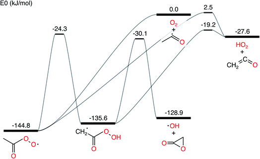 |
| | Fig. 1 Acetyl + O2 potential energy surface using parameters drawn from Allen et al. 2012.11 | |
3.1 Accuracy comparisons
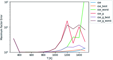
Test fluxes were generated for each of the initial conditions discussed in Sections 2.3 and 2.4, where some of the species were assumed to have c = 0 initially and all the other species were assumed to be in equilibrium. A simulation was run for every possible initial condition of this type for several different temperatures and pressures and all fluxes to species not part of the dominant equilibrium associated with each simulation were added to the test set. The accuracy comparisons were scored using eqn (11) and (12). In most of the figures shown below, the fluxes were evaluated at t = t*, but we also show results from fluxes computed at t = 10t*. One major issue with attempting to analyze the error of these different methods is the fact that unlike SLS, RS, and MSC, the CSE methods do not necessarily satisfy equilibrium. This means that in a mechanism, either the user is using all of the cse rate coefficients and violating equilibrium or they are taking one per reaction in arbitrary directions and reversing them. This is a very important consideration that can be seen in Fig. 2, where best and worst denote the best and worst scoring ways to reverse the rate coefficients, respectively. Interestingly, taking advantage of the lack of equilibrium fluxes in the test set, cse is able to outperform cse_best at high temperatures. One could think about adding equilibrium fluxes to the dataset solely to penalize violation. Mostly equilibrated fluxes so far have not been observed to cause any issues. However, as can be seen in eqn (11), as fluxes get very close to zero, the factor error will explode numerically. If we were to take that direction, the performance of CSE methods would be entirely dependent on how close we wanted to go to equilibrium in the test set. For the remainder of this work, we use the worst scoring directions to reverse cse and cse_g (since the figures are showing worst-case errors).
 |
| | Fig. 2 Scores of raw CSE methods at P = 1 bar. Worst and best denote the worst and best choices of directions in which to force cse to satisfy equilibrium, respectively. The remaining methods do not satisfy equilibrium. Note that cse, unlike cse_g, fails below 500 K. | |
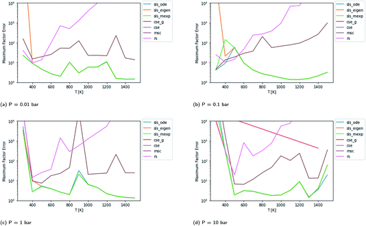
Scores for each method across a wide range of temperatures are presented in Fig. 3. It is worth noting that sls_ode, sls_mexp and sls_eigen all tend to overlap until at low temperatures, where sls_eigen tends to diverge. There is a broad range of conditions where the SLS, CSE, and RS methods are all accurate, but many of the methods significantly mispredict some of the fluxes at high temperature, and some also make large errors at low T.
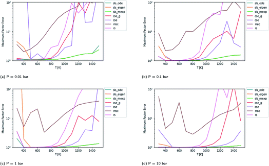 |
| | Fig. 3 Scores for each method at different pressures and temperatures for the acetyl + O2 case study, evaluated at time t*. The scores are the worst-case ratios between the true fluxes and those computed using each method (see eqn (11)). The three SLS methods give identical results under most conditions, and in some cases also agree with the CSE and RS methods, but at low T, methods based on eigendecomposition, such as sls_eigen and cse, often fail. | |
In general, the sls_ode and sls_mexp consistently outperform all other methods in this case study. The occasional deviation between sls_mexp and sls_ode may be a result of optimizing to different minima. In general, below 500 K, sls_ode, sls_mexp, rs, and cse_g perform well. sls_eigen tends to diverge from the other SLS methods as the eigendecomposition becomes less accurate. cse often fails or performs poorly at these temperatures and msc generally performs poorly, although in a fairly consistent manner. In the 500–800 K range, all of the methods except msc perform well. At temperatures greater than 800 K, we see most of the methods diverge. The SLS methods perform significantly better than the other methods in this range. Beyond the SLS methods, the cse and cse_g methods tend to outperform the remaining methods but have difficulties as the reaction and energy transfer timescales get closer together. RS performs poorly in this region as the high temperatures cause larger deviations from Boltzmann distributions within the wells.
In Fig. 4, we examine the same case, except with the isomerization barrier lowered by 20 kcal mol−1. All of the methods mispredict some of the fluxes at some reaction conditions by at least an order of magnitude in this more difficult case. In this case, the CSE methods only succeed occasionally. The RS method has particular difficulties in this case. For this case, under some conditions, the inexpensive and numerically robust MSC method gives smaller maximum errors than some more expensive methods. In this case, the SLS methods again outperform the other methods under most conditions but, like the other methods, SLS wildly mispredicts some of the fluxes at some conditions.
 |
| | Fig. 4 Scores for each method at different pressures and temperatures for the acetyl + O2 case study with the isomerization barrier lowered by 20 kcal mol−1. The CSE methods fail at most conditions in this case. The SLS methods overlap at high temperatures, with sls_eigen diverging at low temperatures. | |
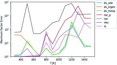
By carefully considering eqn (48) and the definition of p0 in eqn (42)–(44), one can conclude that the test fluxes generated at t* are at least approximately linear combinations of the fluxes the SLS methods were trained on. Given that the phenomenological rate coefficient model we fit to in eqn (5) is also linear, this invites the possibility that the SLS methods are overfitted to the conditions at t*. Testing at higher t* values relaxes some of the chemically significant modes, degrading the diversity of the initial conditions in the test set, but it provides a way to check the SLS-overfitting hypothesis. We provide a representative plot at P = 0.1 bar for 10t* in Fig. 5. While the more relaxed 10t* conditions are much noisier and provide a natural advantage for the RS method, we are able to see that the SLS methods retain similar advantages over the CSE and MSC methods at medium to high temperatures as those seen when using the t* test set. We therefore believe SLS is not overfitted to t* conditions; the SLS training procedure is sufficient for the model to learn the ks corresponding to much slower timescales.
 |
| | Fig. 5 Scores for each method against a test set relaxed to 10t* instead of t* at P = 0.1 bar. | |
Beyond relative performance, however, it is important to take stock of the general performance of prior methods and the overall performance of the master equation methods. Focusing first on Fig. 3, while error does tend to creep up to a factor of 2 at 300 K in some cases, at most temperatures under 800 K the performance tends to be quite good from both the SLS methods and from rs and cse_g. In the 800–1500 K range, however, we see much larger errors. At low pressures in this range, the CSE method errors can be in excess of an order of magnitude. The SLS methods represent a very significant improvement in this region that in many cases achieve in the order of a factor of 5 reduction in the error factor. However, in the P = 0.01 bar case, even the SLS method errors approach factors of 2 or 3, which may be insufficient for some applications.
The overall performance in the case with lower isomerization barriers, however, is much worse. Across the entire temperature range, MSC often hits errors in excess of 2 orders of magnitude, while even the SLS methods often pass above 1 order of magnitude. This is a very troubling level of error that for an important rate coefficient could easily make the difference between whether a chemical kinetic model is viable or not.
An additional important aspect here is what fluxes were the most error prone. While the specific fluxes vary with temperature, the maximum in the factor error, especially for the SLS methods, is usually a flux from a single source condition. Most of the exceptions are at temperatures and pressures where a particular method is performing poorly in general (e.g. due to numerical problems with eigendecomposition).
3.2 Factor error and flux magnitude
In the above analysis of maximum factor error, it is easy to forget the overall context of the fluxes. In Fig. 6, for each flux in the test set for 1300 K and 0.01 bar, we have plotted the predicted flux divided by the largest flux in the associated test simulation against the factor error in the predicted flux. Since the SLS and CSE methods largely had the same behavior, we only plotted one of each type of method. We can see that for the SLS and CSE methods, the vast majority of fluxes have very small factor errors. We can also see that each method has a different relationship with the scaled flux. As might be expected, SLS factor errors are largely flat near one, having no relationship with the scaled flux. MSC factor errors vary a whole lot but have no clear correlation with the scaled flux. RS tends to generally have higher errors at lower scaled fluxes; although the relationship is not entirely clear. CSE errors, on the other hand, clearly increase with decreasing scaled flux below 10−3. This suggests to us that for the CSE methods, the large maximum error factors observed may tend to be associated with smaller fluxes, as one might expect.
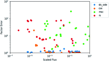 |
| | Fig. 6 Scatter plot of the predicted value of the flux divided by the largest flux from its associated test simulation against the factor error in the predicted flux at 1300 K and 0.01 bar. | |
3.3 Rate coefficients
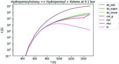
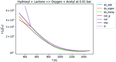
In general, many of the computed phenomenological rate coefficients agree quite well between all of the methods. Two exceptions are shown in Fig. 7 and 8. One can see that even in this pair of rate coefficients selected to show differences, all of the methods largely converge at low and high temperatures, respectively.
 |
| | Fig. 7 Rate coefficient for hydroperoxylvinoxy to hydroperoxyl and ketene at 0.1 bar. | |
 |
| | Fig. 8 Rate coefficient for hydroxyl and lactone to oxygen and acetyl at 0.01 bar. | |
3.4 Neglecting collisions at high energy
The application of eqn (52) to improve the conditioning of the master equation matrix did not provide any consistent accuracy gains, as can be seen in Fig. 9. This method at εtol = 0.1 did cause CSE to be able to successfully generate rate coefficients at 300 K, 1 bar and 400 K, 10 bar, giving quite reasonable scores. Without this approach, it was unable to do so. However, overall, this approximation does not seem to result in any consistent accuracy benefits.
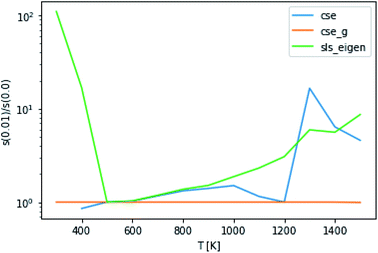 |
| | Fig. 9 Ratio of scores using an energy tolerance of 0.01 to scores without at P = 0.1 bar. Above and below 1 denote worse and better scores from s(0.01), respectively. | |
This technique drastically reduces the condition number of the matrix, as can be seen in Fig. 10. However, the maximum condition number of the eigenvalues and the maximum separation of the eigenvalues (an analog to condition number for eigenvectors), excepting the highest and lowest temperatures, remain virtually constant.14
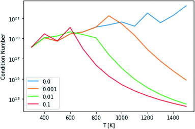 |
| | Fig. 10 Condition numbers of the master equation matrix at P = 1.0 bar at different high energy rate tolerances. | |
3.5 Examining error in the CSE method
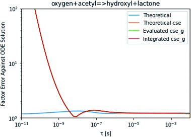
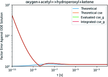
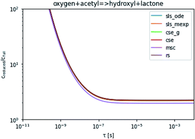
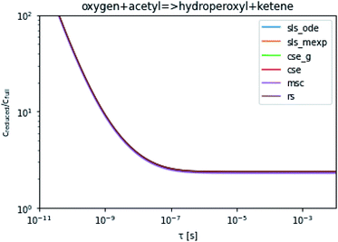
To take a closer look at errors within the cse method, we analyzed eqn (17) with r˙ = acetyl and B = O2 for the radical decay case  at P = 0.01 bar and T = 500 K. We generated a benchmark solution by simulating eqn (17) numerically. We then calculated the bimolecular–bimolecular fluxes starting from oxygen + acetyl at each time using the ode solution, the exact theoretical solution from eqn (33) and (34), by simply evaluating the cse_g rate coefficients at the concentrations given from the ode solution and by integrating the cse_g rates. The results, as a function of τ = t, are presented in Fig. 11 and 12. We also looked at the ratio of the product concentrations between the reduced models and the benchmark solution. These are presented in Fig. 13 and 14.
 |
| | Fig. 11 Factor error in the flux from oxygen + acetyl in the decay case to hydroxyl + lactone at 0.01 bar and 500 K for t = τ between a benchmark ODE solution of eqn (17) and the theoretical solution from eqn (33), theoretical cse from eqn (34), cse_g evaluated at the benchmark, and integrated cse. | |
 |
| | Fig. 12 Factor error in the flux from oxygen + acetyl in the decay case to hydroperoxyl + ketene at 0.01 bar and 500 K for t = τ between a benchmark ODE solution of eqn (17) and the theoretical solution from eqn (33), theoretical cse from eqn (34), cse_g evaluated at the benchmark, and integrated cse. | |
 |
| | Fig. 13 Ratio of the hydroxyl or lactone concentrations between the reduced and benchmark simulations in the decay case at 0.01 bar and 500 K for t = τ. | |
 |
| | Fig. 14 Ratio of the hydroperoxyl or ketene concentrations between the reduced and benchmark simulations in the decay case at 0.01 bar and 500 K for t = τ. | |
At long times, we observe almost no difference between the theoretical exact and theoretical cse fluxes. This tells us that the primary assumption of cse, that the energy modes can be assumed to be at steady state, is very good. The appreciable factor errors at long times between the ode solution and the other methods, particularly the other exact solution eqn (33), suggest that the error in cse methods has a significant component associated specifically with the eigendecomposition and not associated with the dimensionality reduction operation. This long time error appears in the concentration plots as a factor error in the concentration that persists after the energy modes have relaxed.
At short times, we see that once τ gets below around 10−8 s, the error for every method except the theoretically exact formula starts to increase dramatically as the timescale is decreased. At a 10−9 s timescale, the flux factor error hits 2, becoming difficult to neglect in simulations. In the concentration plots, we see that the errors in fluxes induce errors in the concentrations that persist out farther than the flux errors themselves to about 10−7 seconds. At a timescale of 10−8 seconds in this system, we might expect the standard reduced model in eqn (5) to predict product concentrations that are 3× higher than those that might be predicted by a full model. At 10−9 seconds, this factor of 3 increases to a factor of 7–20, depending on the product.
3.6 Computational cost
Table 1 contains the time required to generate the data for each method in Fig. 3. There are many nuances to the implementations, however. The cse, msc, and rs methods are the highly optimized Cython implementations from Allen et al. 2012. The sls methods and cse_g are comparatively unoptimized pure Python implementations. The sls_ode method generates Julia derivative and jacobian functions and calls Julia on them to solve the ODE. While this makes the solution very fast, it adds a jit compiling overhead for those functions once per temperature/pressure condition that we have seen some evidence may be limiting the performance.
Table 1 Total time required to generate plots for each method in Fig. 3
| Method |
Time (s) |
| sls_ode |
719.83 |
| sls_eigen |
19.25 |
| sls_mexp |
17.33 |
| cse_g |
33.36 |
| cse |
23.60 |
| msc |
9.82 |
| rs |
10.40 |
One major observation here is that all of these times are much shorter than the time required to run the quantum chemistry calculations needed to define the network. Another is that sls_mexp, even at the current optimization level, is marginally faster than Arkane’s cythonized cse implementation. Lastly and perhaps most interestingly, the relative speeds of cse, msc, and rs here heavily disagree with those reported by Allen et al. 2012, despite the fact that we are using the exact implementations from that paper on the exact same network. This is most likely a result of the fact that Allen et al. 2012 seems to have included computations in the range of roughly 10−4 to 104 bar and 300 to 2000 K, while our Fig. 3 only ranges from 10−2 bar to 101 bar and 300 to 1500 K. Allen et al. 2012, from their results, suggested that msc was a factor of 2 faster than rs and that msc was a factor of roughly 62 times faster than cse, while we here show msc and rs being about the same speed and only being about a factor of 2 faster than cse. A range of 10−2 bar to 102 bar and 300 K to 2000 K may be more typical conditions for fitting than either case. Our set of conditions are likely most similar to that, so our timing ratios may be more typical than those presented in Allen et al. 2012.
4. Discussion
Applications for master equation reduction algorithms tend to differ in two primary ways: whether the parameters are estimated from quantum chemistry or using faster methods and whether or not the algorithm is run automatically or by hand. Perhaps the most common case is running quantum chemistry calculations and the master equation reduction algorithm by hand. In this context, accuracy is much more important than speed and robustness. But master equation reduction has also found important applications in automatic pressure dependent mechanism generation, such as that in RMG.11,15,16 In these contexts, it is most important to have a robust and fast master equation reduction algorithm. Additionally, with many new workflows for the automatic running of quantum chemistry calculations,17–19 it will likely be important soon to consider carefully the case when the algorithm needs to run automatically with quantum chemistry calculations. In that particular case, it will likely be of interest to achieve high accuracy in a robust manner.
The CSE method for a long time has been considered by many to be the most accurate master equation reduction method. However, it has always had two primary weaknesses. At low temperatures, the accuracy of the eigendecomposition becomes problematic, causing it to fail and become inaccurate. At high temperatures, the method breaks down as the energy and reaction eigenvalues get too close. Methods have been developed to handle the latter by combining species into one well.8 However, while this is the most correct way to handle the situation, the tactic of combining species presents many difficulties in chemical mechanism development. In this work, we see in Fig. 3 that the cse_g method seems to alleviate much of the trouble the cse method has with low temperature robustness and accuracy at the conditions examined. However, these methods seem to perform significantly worse than expected, especially at higher temperatures.
The sls_ode and sls_mexp methods developed here are highly accurate and robust. The limited conditions they fit to are usually their highest error conditions in our diverse test set. In our examination here, they nearly always outperform every other method in terms of accuracy. The sls methods also do not have the same issues the cse methods do with well merging. As an eigenmode associated with motion between the wells becomes buried under energy transfer eigenvalues, as defined currently, t* will become defined by the slowest energy transfer eigenvalue. The simulations will then start to relax the motions between the merged wells. This will mostly decouple the rate coefficient parameter associated with the motion between them from the other rate coefficients. As a result, fluxes in the fitting set between the merging wells will become mostly equilibrated. While this does not provide the best leverage for fitting the rate coefficient under the conditions of interest, we only need a reasonable value, and so far we have yet to see that these mostly equilibrated fluxes have a significant impact on the error of the SLS methods. However, the problem is not entirely resolved because we are no longer fully relaxing the slowest energy transfer mode. This issue would be easily resolved with a robust technique for determining which eigenvalues are chemically significant and which are associated with energy transfer in cases where they are not separated, but as far as the authors are aware, such a technique has yet to be developed. Regardless, the SLS methods are able to handle this issue with somewhat reduced accuracy.
In terms of robustness, all of the SLS methods are dependent on the calculation of the eigenvalues of the master equation matrix and the determination of the fastest reaction timescale; however, they are not dramatically sensitive to the accuracy of the determined timescale t*. Additionally, sls_ode is dependent on the success of the ODE solve. We have yet to observe cases where the ODE solve actually fails, but we have observed some cases where the solve can take quite a long time. For this reason, sls_mexp may be a better choice for applications that require robustness.
The highly variable levels of accuracy seen in this work for master equation reduction methods as a function of network, temperature, and pressure suggest that we are in need of improved techniques for estimating uncertainty in the reduced models. The error analysis introduced in this paper benchmarking fluxes against the ODE solution provides one method. However, the test set for this method scales exponentially with the number of reactant and isomer channels and it may be impractical for larger and stiffer networks. In these cases, one may instead adopt the linear scaling subset and faster simulation techniques used in the SLS methods. Ideally, one would compare the benchmark and reduced fluxes overall or just for those that are most similar to situations of interest. However, we appreciate that when applied to large scale mechanism development, this analysis can be quite tedious and inconvenient to combine with existing rate coefficient associated uncertainties. At least for the SLS methods, one could imagine expanding the least-squares objective function around the minimum and applying a suitable weighting function to generate a joint distribution of the phenomenological rate coefficients. More generally, however, ignoring the fact that the phenomenological rate coefficients for a network are correlated and their uncertainties jointly distributed and neglecting any errors in the benchmark simulations, using eqn (51) we can write approximately
| |  | (53) |
where
ui→j(
T,
P) is the factor uncertainty in the rate coefficient from
i →
j associated with master equation reduction,
ϕsinglesource,i,→jfull(
T,
P) is the benchmark single source flux from
i →
j, and
ϕsinglesource,i,→jred(
T,
P) is the same flux for the reduced model. Note that this is obtained virtually for free for the SLS methods.
For non-automated applications, we recommend use of the sls_ode and/or sls_mexp methods. These methods are highly accurate. For automated applications on long time scales, such as those involving automated quantum chemistry calculations, we recommend the use of sls_mexp, which is accurate and robust. For automatic pressure dependent mechanism generation applications, recommendations are a bit trickier. Allen et al. 2012 recommended the use of MSC for these applications because while they found RS to be accurate on the same system examined here, they found that when they lowered the barriers, RS became appreciably less accurate. They also found that cse was too slow and not robust enough for the application. sls_mexp should be robust enough to use for this application; however, we are uncertain about how well sls_mexp might scale with network size. Unlike MSC and RS, sls_mexp has to generate the full master equation matrix, calculate its eigenvalues, and then calculate the matrix exponential, all of which scale nonlinearly with network size.
Fig. 3 demonstrates that even in the easier case at low pressure, it is highly difficult to consistently perform better than a factor error of 1.5. In the harder case in Fig. 4, even at high temperatures it is difficult to consistently perform better than a factor error of 10, let alone at lower temperatures. Looking at fast timescale experiments where a radical decays rapidly, causing its concentration to vary faster than energy transfer timescales, we can see in Fig. 13 and 14 that existing methods are insufficient to accurately predict product concentrations. Similar effects might be seen in shock tube conditions where the temperature changes more quickly than the energy transfer timescale. Under these kinds of conditions, we suspect that the current reduced model, as defined in eqn (5), may be insufficient. There are many alternative reduced models we might consider. However, a major barrier is how we might define the parameters for such a model robustly. While the important conditions, the initial guesses, and the simulation time may need modification depending on the model choice, the principle of the SLS technique should be flexible to these sorts of advanced models.
5. Conclusions
Here, we have presented a flux-based analysis of the error in master equation reduction techniques. We have developed simulation-least squares, a new fitting based technique for master equation reduction. This method performs very well in terms of speed and accuracy and we believe it should be considered alongside existing well-established methods. We have examined the possibility of removing coupling associated with collisions for high energy grains within the master equation to improve performance. However, while the principle of that assumption seems to work well, we were unable to observe consistent accuracy or robustness improvements. Lastly, we have taken an in depth theoretical and numerical look at the time dependent error of the popular CSE based methods.
Author contributions
WHG and MSJ each conceived of different portions of this work. All of the computer programming and simulations and most of the writing was done by MSJ. Both authors contributed to the interpretations and clarifying the presentation.
Conflicts of interest
There are no conflicts to declare.
Acknowledgements
We gratefully acknowledge the financial support for this work from the Gas Phase Chemical Physics Program of the U.S. Department of Energy, Office of Basic Energy Sciences, Division of Chemical Sciences, Geosciences, and Biosciences under Award number DE-SC0014901.
Notes and references
- B. M. Wong, D. M. Matheu and W. H. Green, J. Phys. Chem. A, 2003, 107(32), 6206–6211 CrossRef CAS.
- A. Chang, J. Bozzelli and A. Dean, Z. Phys. Chem., 2000, 214, 1533 CAS.
- N. J. B. Green and Z. A. Bhatti, Phys. Chem. Chem. Phys., 2007, 9, 4275 RSC.
- J. R. Barker, Int. J. Chem. Kinet., 2001, 33, 232–245 CrossRef CAS.
- J. T. Bartis and B. Widom, J. Chem. Phys., 1974, 60, 3474–3482 CrossRef CAS.
- S. J. Klippenstein and J. A. Miller, J. Phys. Chem. A, 2002, 106(40), 9267–9277 CrossRef CAS.
- J. A. Miller and S. J. Klippenstein, J. Phys. Chem. A, 2006, 110(36), 10528–10544 CrossRef CAS PubMed.
- Y. Georgievskii, J. A. Miller, M. P. Burke and S. J. Klippenstein, J. Phys. Chem. A, 2013, 117, 12146–12154 CrossRef CAS PubMed.
- D. R. Glowacki, C.-H. Liang, C. Morley, M. J. Pilling and S. H. Robertson, J. Phys. Chem. A, 2012, 116, 9545–9560 CrossRef CAS PubMed.
-
A. G. Dana, M. S. Johnson, J. W. Allen, S. Sharma, S. Raman, M. Liu, C. W. Gao, C. A. Grambow, M. J. Goldman, D. S. Ranasinghe, R. J. Gillis, A. M. Payne, Y.-P. Li, E. E. Dames, Z. J. Buras, N. M. Vandewiele, N. W. Yee, S. S. Merchant, B. Buesser, C. A. Class, C. F. Goldsmith, R. H. West and W. H. Green, Automated Reaction Kinetics and Network Exploration (Arkane), 2022, https://github.com/ReactionMechanismGenerator/RMG-Py Search PubMed.
- J. W. Allen, C. F. Goldsmith and W. H. Green, Phys. Chem. Chem. Phys., 2012, 14, 1131–1155 RSC.
- C. Rackauckas and Q. Nie, J. Open Res. Software, 2017, 5(1), 15 CrossRef.
- A. H. Al-Mohy and N. J. Higham, SIAM J. Matrix Anal. Appl., 2010, 31, 970–989 CrossRef.
- C. Van Loan, Linear Algebra Appl., 1987, 88–89, 715–732 CrossRef.
- C. W. Gao, J. W. Allen, W. H. Green and R. H. West, Comput. Phys. Commun., 2016, 203, 212–225 CrossRef CAS.
- M. Liu, A. Grinberg Dana, M. S. Johnson, M. J. Goldman, A. Jocher, A. M. Payne, C. A. Grambow, K. Han, N. W. Yee, E. J. Mazeau, K. Blondal, R. H. West, C. F. Goldsmith and W. H. Green, J. Chem. Inf. Model., 2021, 61, 2686–2696 CrossRef CAS PubMed.
-
A. G. Dana, D. Ranasinghe, O. H. Wu, C. Grambow, X. Dong, M. Johnson, M. Goldman, M. Liu and W. H. Green, ARC - Automated Rate Calculator, version 1.1.0, 2019, GitHub, DOI:10.5281/zenodo.3356849, https://github.com/ReactionMechanismGenerator/ARC.
-
J. Zádor and J. A. Miller, Proceedings of the Combustion Institute, 2015 Search PubMed.
- R. Van de Vijver and J. Zádor, Comput. Phys. Commun., 2020, 248, 106947 CrossRef CAS.
Footnote |
| † Electronic supplementary information (ESI) available. See DOI: 10.1039/d2fd00040g |
|
| This journal is © The Royal Society of Chemistry 2022 |
Click here to see how this site uses Cookies. View our privacy policy here.  Open Access Article
 and
William H.
Green
 *
*


 , giving us


 . We can use this to cleanly scale the flux error


 and
and  for the energy transfer associated eigenvalues, giving us


 , the error is the same as that of the steady state concentration case; however, when τ is small the error gets much more interesting. The first thing of note is the λiτ = −1 singularity; however, examining the particular factor in eqn (37), we get


 . This relative error can be significant for strongly chemically-activated cases, where zi can be large for some of the high eigenvalues, and some of the corresponding microcanonical reaction rates represented by gCD can be much larger in magnitude than some of the λis.


 at P = 0.01 bar and T = 500 K. We generated a benchmark solution by simulating eqn (17) numerically. We then calculated the bimolecular–bimolecular fluxes starting from oxygen + acetyl at each time using the ode solution, the exact theoretical solution from eqn (33) and (34), by simply evaluating the cse_g rate coefficients at the concentrations given from the ode solution and by integrating the cse_g rates. The results, as a function of τ = t, are presented in Fig. 11 and 12. We also looked at the ratio of the product concentrations between the reduced models and the benchmark solution. These are presented in Fig. 13 and 14.
